
Chapter 17
Ambient Occlusion
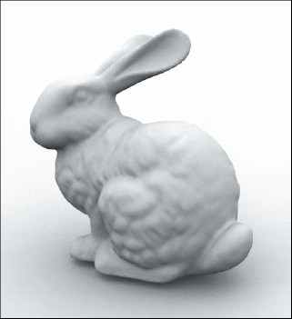
Image courtesy of Mark Howard, Stanford bunny model courtesy of Greg Turk and the Stanford University Graphics Laboratory
Objectives
By the end of this chapter, you should:
- understand how ambient occlusion is computed;
- know how to set up a local orthonormal basis at a hit point;
- have implemented ambient occlusion as a light shader;
- understand some of the limitations of the sampling techniques discussed in Chapter 5.
In Chapter 14, ambient illumination was a constant term throughout a scene. As a result, the surface of any object that only received ambient illumination was rendered with a constant color. Ambient occlusion can significantly increase the realism of the ambient illumination in ray-traced images. The idea is quite simple: the amount of ambient illumination received at a surface point depends on how much of the hemisphere above the point is not blocked (occluded) by objects. Figure 17.1 illustrates this in two dimensions for a scene that consists only of a sphere and a box. Because the box isn’t visible from point a on the sphere, a receives ambient light from the whole hemisphere, which is the maximum amount. In contrast, the box is visible from the point b and blocks some of the incoming ambient illumination, so b does not receive the maximum amount.
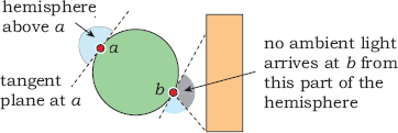
Point a on the sphere receives the maximum amount of ambient light because the box isn’t visible; point b doesn’t receive the maximum amount because the box blocks some of the incoming ambient light.
Ambient occlusion is still an approximation of diffuse-diffuse light transport. For example, point b can also receive diffuse illumination that’s been reflected from the box, but I’ll ignore that here. It’s computed in Chapter 26.
17.1 Modeling
We can model ambient occlusion by including a visibility term in Equation (14.1) for the incident ambient radiance. The new expression for the incident radiance is
where Li now depends on p and ωi. The visibility term is
As a result, Li(p, ωi) is a binary-valued function: either black or ls cl, depending on ωi. The only practical way to estimate the ambient illumination (17.1) is to shoot shadow rays into the hemisphere above p and see how many of them hit objects. We can make the ambient illumination for a given pixel proportional to the number of rays that don’t hit objects, but how do we distribute the rays? You may think that the best way is a uniform distribution in solid angle. While that would be the best way to estimate the solid angle occluded by the objects, it’s not quite what we need. The reason is Lambert’s law, as discussed in Section 13.2. This results in the irradiance being proportional to the cosine of the polar angle θi at p.
We have to estimate the integral (13.10) for the reflected radiance
Using Equation (13.19) for fr = fr,d = kdcd/π with ka instead of kd, and Equation (17.1) for Li(p, ωi), we have
Recall from the discussion of Monte Carlo integration in Section 13.11 that the best estimate for an integral is obtained by using a sample density that matches the integrand. Because of the cos θi in the integrand, we should therefore shoot the shadow rays with a cosine distribution in the polar angle. As the distribution of objects is unknown, the cosine is the only thing we know about the integrand.
Before we can shoot a shadow ray, we have to set up an orthonormal basis at p, where w is in the direction of the normal at p. Figure 7.4 shows an orthonormal basis set up in this way. Because the orientation of u and v around w doesn’t matter, we can use the following construction for (u, v, w):
In practice, it’s a good idea to jitter the up vector, in case the surface being shaded is horizontal (see Listing 17.2). Because we only shoot one shadow ray per primary ray, this orthonormal basis will have to be set up for every ray. Provided we have samples on a hemisphere with a cosine distribution, the ray direction for a given sample point s = (sx, sy, sz) is
which simply projects the 3D sample point onto u, v, and w. By construction, d is a unit vector. Refer to Sections 7.1 and 7.2 to see how the sample points are set up on the hemisphere.
17.2 Implementation
There are two ways we can implement ambient occlusion. One is through a material that’s responsible for sampling the hemisphere. Although there’s nothing wrong with this approach, we would have to use the material with every object for which we wanted the effect. Since we already have two materials
class AmbientOccluder: public Light {
public:
AmbientOccluder(void);
...
void
set_sampler(Sampler* s_ptr);
virtual Vector3D
get_direction(ShadeRec& sr);
virtual bool
in_shadow(const Ray& ray, const ShadeRec& sr) const;
virtual RGBColor
L(ShadeRec& sr);
private:
Vector3D u, v, w;
Sampler* sampler_ptr;
RGBColor min_amount;
};
Listing 17.1. Declaration for the class AmbientOccluder.
with an ambient-reflection component, it would be nice to get ambient occlusion working with these without having to change them and without having to add a new material. Fortunately, this is possible by using a light shader. By building ambient occlusion into a new ambient light, it will work for any material that has an ambient-reflection component. All we have to do is use the new light in place of the existing constant ambient light. Listing 17.1 shows the class declaration for the new light, which I’ve called AmbientOccluder.
The member function set_sampler appears in Listing 17.2.1 This function assigns the sampler sp (constructed in the build functions) and then maps the samples to the hemisphere with a cosine (e = 1) density distribution. Recall from Chapter 5 that when a sampler object is constructed, the samples are only generated in the unit square; it’s always the application code’s responsibility to distribute them over a hemisphere when required.
void
AmbientOccluder::set_sampler(Sampler* s_ptr) {
if (sampler_ptr) {
delete sampler_ptr;
sampler_ptr = NULL;
}
sampler_ptr = s_ptr;
sampler_ptr->map_samples_to_hemisphere(1);
}
Listing 17.2. The function AmbientOccluder::set_sampler.
Vector3D
AmbientOccluder::get_direction(ShadeRec& sr) {
Point3D sp = sampler_ptr->sample_hemisphere();
return (sp.x * u + sp.y * v + sp.z * w);
}
Listing 17.3. The function AmbientOccluder::get_direction.
Listing 17.3 shows the function get_direction, which returns the direction of each shadow ray. Notice that this function simply projects the components of the local variable sp onto (u, v, w), as in Equation (17.4).
To test if a shadow ray is blocked by an object, we can use a standard in_shadow function. The in_shadow function in Listing 17.4 is the same as that for a directional light.
bool
AmbientOccluder::in_shadow(const Ray& ray, const ShadeRec& sr) const {
float t;
int num_objects = sr.w.objects.size();
for (int j = 0; j < num_objects; j++)
if (sr.w.objects[j]->shadow_hit(ray, t))
return (true);
return (false);
}
Listing 17.4. The function AmbientOccluder::in_shadow.
RGBColor
AmbientOccluder::L(ShadeRec& sr) {
w = sr.normal;
// jitter up vector in case normal is vertical
v = w ^ Vector3D(0.0072, 1.0, 0.0034);
v.normalize();
u = v ^ w;
Ray shadow_ray;
shadow_ray.o = sr.hit_point;
shadow_ray.d = get_direction(sr);
if (in_shadow(shadow_ray, sr))
return (min_amount * ls * color);
else
return (ls * color);
}
Listing 17.5. The function AmbientOccluder::L.
Finally, the function AmbientOccluder::L in Listing 17.5 illustrates how the orthonormal basis is set up and how the functions get_direction and in_shadow are called. Note that L sets up (u, v, w) before it calls get_ direction, where these are used.
I use the data member min_amount to return a minimum non-black color when the ray direction is occluded because this results in more natural shading than returning black. It takes into account the fact that all surfaces in real scenes receive some light. The figure on the first page of this chapter and the figures in Section 17.5 demonstrate the benefits of this approach.
All we have to do to get ambient occlusion working is to construct an AmbientOccluder light in a build function and assign it to the world’s ambient light.
17.3 A Simple Scene
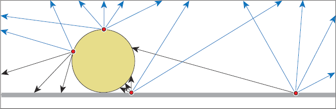
I’ll consider here a simple test scene that consists of a plane and a sphere that just touch. Figure 17.2 illustrates how the ambient illumination varies over the surfaces of both objects. Arrows at the hit points are shadow rays, which either don’t hit anything (blue) or hit one of the objects (black). As points on the plane get closer to the sphere, the solid angle it subtends increases, more shadow rays hit it, and the ambient illumination that the points receive decreases. A similar situation applies to the sphere. The farther from the top a hit point is, the less ambient illumination it receives.
Listing 17.6 is the build function, which demonstrates how to construct an AmbientOccluder light that uses multi-jittered sampling.
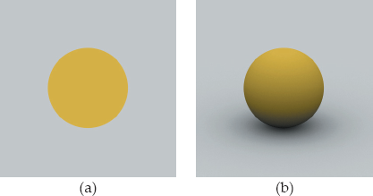
The following images show this scene rendered with various sampling techniques but using only ambient illumination. Figure 17.3(a) was rendered with constant ambient illumination, which provides little information about the scene. Figure 17.3(b) shows the scene as it “should” appear with ambient occlusion. This part was rendered with multi-jittered sampling and 256 rays per pixel. Notice how the ambient occlusion provides a rounded appearance for the sphere and relates it to the plane, like shadows do. Figure 17.3(b) uses min_amount = 0, as do Figures 17.4, 17.6, and 17.7, because this value is best for demonstrating the differences between sampling techniques.

Sphere and plane scene rendered with constant ambient illumination (a) and ambient occlusion (b).
void
World::build(void) {
int num_samples = 256;
vp.set_hres(400);
vp.set_vres(400);
vp.set_samples(num_samples);
tracer_ptr = new RayCast(this);
MultiJittered* sampler_ptr = new MultiJittered(num_samples);
AmbientOccluder* occluder_ptr = new AmbientOccluder;
occluder_ptr->scale_radiance(1.0);
occluder_ptr->set_color(white);
occluder_ptr->set_min_amount(0.0);
occluder_ptr->set_sampler(sampler_ptr);
set_ambient_light(occluder_ptr);
Pinhole* camera_ptr = new Pinhole;
camera_ptr->set_eye(25, 20, 45);
camera_ptr->set_lookat(0, 1, 0);
camera_ptr->set_view_distance(5000);
camera_ptr->compute_uvw();
set_camera(camera_ptr);
Matte* matte_ptr1 = new Matte;
matte_ptr1->set_ka(0.75);
matte_ptr1->set_kd(0);
matte_ptr1->set_cd(1, 1, 0); // yellow
Sphere* sphere_ptr1 = new Sphere (Point3D(0, 1, 0), 1);
sphere_ptr1->set_material(matte_ptr1);
add_object(sphere_ptr1);
Matte* matte_ptr2 = new Matte;
matte_ptr2->set_ka(0.75);
matte_ptr2->set_kd(0);
matte_ptr2->set_cd(1); // white
Plane* plane_ptr1 = new Plane(Point3D(0), Normal(0, 1, 0));
plane_ptr1->set_material(matte_ptr2);
add_object(plane_ptr1);
}
Listing 17.6. The build function for Figure 17.3(b). You can also use this build function to render Figures 17.4, 17.6, and 17.7 by using different numbers of samples and assigning a different sampling technique to the ambient occluder’s sampler pointer.

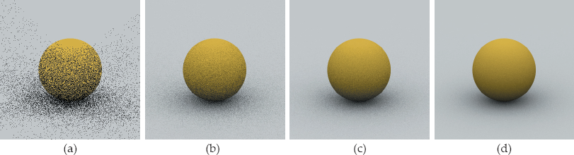
Scene rendered using regular sampling with one sample per pixel (a), 16 samples (b), 64 samples (c), and 256 samples (d).
Ambient occlusion is much better than antialiasing or depth of field for exposing the shortcomings of sampling techniques, as Figure 17.4 illustrates. This figure shows the sphere scene rendered using regular sampling with different numbers of samples per pixel. As you can see, these images are not even approximately correct, although Figure 17.4(d) may appear all right until you look at the image on the book’s website. So, what’s gone wrong? First, there’s only a single set of regular samples to work with (for a given number of samples), so we get correlations. Second, and more importantly, the sample points are mapped onto regular patterns on the hemisphere, as Figure 17.5 illustrates for 256 samples. Even with this large number, there are only 16 evenly spaced azimuth angles used and 16 polar angles. This creates the bands on the sphere and the patterns on the plane (see Question 17.5). Hammersley sampling produces similar results, and for the same reasons. The lesson here is that although uniformly distributed samples are good, regularly spaced samples are not good.
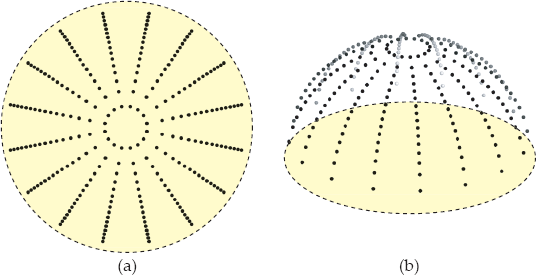
(a) 256 regular samples mapped to a hemisphere with a cosine distribution; (b) 3D view of the samples.
Figures 17.6 and 17.7 show, respectively, random and multi-jittered sampling using the same numbers of sample points.

Figures 17.6(a) and 17.6(b) show how noisy the results are with one sample per pixel, but that’s understandable because, in general, the wider the angular range of the samples, the more samples you need to reduce noise to acceptable levels. Ambient occlusion is as wide as you can get—the whole hemisphere above each hit point.
The images also illustrate another point: ambient occlusion is black with one ray per pixel. Shades of gray only appear with multiple rays.
Unfortunately, the printed images here can’t show you the most important feature: multi-jittered sampling produces results with 64 samples that are as good as random sampling produces with 256 samples. You have to look at the images on the book’s website to see this, where it’s obvious. The reason is the superior 1D and 2D distributions of the multi-jittered samples.
Jittered sampling gives better results than random, but not as good as multi-jittered, and n-rooks gives results that are similar to random sampling. We can draw the following conclusions from these images:
- Regular sampling is unsuitable for ambient occlusion because of the regular 1D distributions of samples. This results in obvious aliasing artifacts. Hammersley sampling is also unsuitable for the same reasons.
- For this application, multi-jittered sampling is the best of the techniques discussed in Chapter 5 because it allows us to get similar results to random sampling with about one-quarter of the number of samples. That’s an important saving in view of the large number of samples that we need in general.
Because we usually render scenes with lights and direct illumination, Figure 17.8 shows the scene illuminated with a directional light. Here, I’ve decreased the ambient-reflection coefficients for the sphere and plane to stop the direct illumination from washing out the images.
Modified scene rendered with direct illumination from a directional light and constant ambient illumination (a) and with direct illumination and ambient occlusion (b). Multi-jittered sampling was used for the antialiasing and the ambient occlusion, with 100 samples per pixel.
17.4 Two-Sided Objects
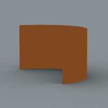
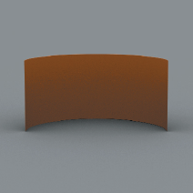
In Section 14.6.2, I discussed the issues involved in correctly shading both sides of surfaces with direction illumination. Although these issues don’t apply to constant ambient illumination, they do apply to ambient occlusion. The reason is that the shadow rays are shot into the hemisphere around the normal. As an example, Figure 17.9 shows a half cylinder rendered with incorrect ambient illumination, where both sides of the cylinder are the same color.
The problem is the outward-pointing normal to the cylinder, as shown in Figure 17.10(a). If there were no other objects in the scene, both sides of the cylinder would be rendered with full ambient illumination, as illustrated by points a and b, because none of the shadow rays would hit anything. In reality, some shadow rays from points on the inside surface will hit the cylinder, as illustrated by point b in Figure 17.10(b). According to Section 14.6.2, a solution is to use an object whose hit function reverses the normal when a ray hits the inside surface.
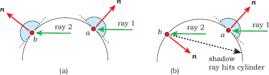
Ray 1 hits the outside surface of a cylinder at a, and ray 2 hits the inside surface at b. (a) The normal points outwards at both hit points. (b) The normal points inwards at point b, and some of the shadow rays will hit the cylinder.
Figure 17.11(a) shows the correct ambient-occlusion shading with a two-sided half cylinder; Figure 17.11(b) shows the scene rendered with direct illumination added.
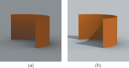
A half cylinder rendered with correct ambient occlusion (a) and with ambient occlusion and direct illumination (b).
The same situation applies to other open curved objects. Question 17.6, Question 17.7 and Question 17.8 are relevant to these shading issues.
17.5 Other Scenes
Figure 17.12 shows the Stanford bunny rendered with three values of min_amount. In Figure 17.12(a), min_amount = 1.0, and this image is therefore the same as we would get with constant ambient illumination.2 In Figure 17.2(b), min_amount= 0.25, and in Figure 17.12(c), min_amount= 0.0. Notice that although the images become darker as min_amount decreases, the contrast increases.
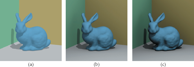
Bunny scene rendered with 256 samples per pixel: (a) min_amount = 1; (b) min_amount = 0.25; (c) min_amount = 0.
Figure 17.13 shows similar effects with the random boxes used in the viewing chapters. Again, notice the difference in contrast in Figure 17.13(a) and (b).
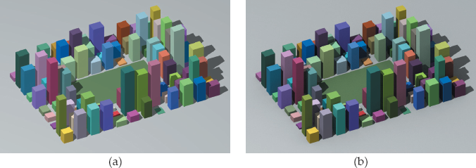
Random boxes rendered with 64 samples per pixel: (a) min_amount = 1.0; (b) min_amount = 0.25.
I’ve found that for most scenes, min_amount = 0.25 provides a good balance between the constant ambient look of min_amount = 1.0 and the equally unnatural-looking black areas that result from using min_amount = 0.0. You should experiment.
Notes and Discussion
Most objects that use samples have a set_sampler function and a set_samples function. The set_sampler function allows a pointer to any type of sampler to be assigned to an object, and it also performs any required mapping of the samples to a disk or a hemisphere. This is the appropriate function to use here because an important function of this chapter is to compare the results of different sampling techniques for ambient occlusion.
The set_samples function constructs a default sampler object with the specified number of samples. AmbientOccluder::set_samples constructs a multi-jittered sampler object for all (perfect-square) values of num_samples. This gives random samples when there is one ray per pixel, in contrast to ViewPlane::set_samples, which constructs a uniform sampler when num_ samples = 1. Performing ambient occlusion with one ray per pixel then results in noisy images such as Figure 17.6(a) instead of images like Figure 17.4(a). You can, of course, decide which you prefer and write the AmbientOccluder:: set_samples function accordingly.
Further Reading
There hasn’t been much written about ambient occlusion. I don’t know of any other ray-tracing textbooks that discuss it. It was implemented in RenderMan in about 2002, and I’ve got most of my information about it from online RenderMan documentation. There’s a Wikipedia article at http://www.wikipedia.org/wiki/Ambient_occlusion, which includes links.
Questions
- 17.1. Consider a scene that consists of a single closed object. Can ambient occlusion be relevant?
- 17.2. Consider a completely closed environment such as the random boxes scene in Figures 11.11 and 11.12, which includes a sky-dome hemisphere. How can you get ambient occlusion to work in this case?
- 17.3. Why is d a unit vector in Equation (17.4)?
- 17.4. In Figure 17.2, what fraction of the sphere’s surface receives full ambient illumination?
- 17.5. In Figure 17.4, can you see a relationship between the number of uniform samples used and the number of “spokes” on the plane?
- 17.6. In Figure 17.11(a), the surface of the cylinder is perpendicular to the plane, and there are no other objects in the scene. Why is the outside surface of the cylinder rendered with a constant color?
- 17.7. Figure 17.14 shows another view of the cylinder where we can see all of the inside surface. Why does the ambient shading vary from top to bottom, but not horizontally? What fractions of the total ambient illumination do points receive along the top and bottom inside edges of the cylinder?
- 17.8. Do the shading issues discussed in Section 17.4 apply to planar objects such as rectangles, disks, and triangles?
- 17.9. The rectangles in Figure 17.12 meet at a corner behind the bunny with coordinates (-0.13, 0.033, -0.1). Figure 17.15 was rendered with the pinhole camera parameters
float delta = 0.01camera_ptr->set_eye(-0.13 + delta, 0.033 + delta, -0.1 + delta);camera_ptr->set_lookat(1.0, 0.5, 1.0);camera_ptr->set_view_distance(100.0);which is just inside the corner looking out, min_amount = 0.0, and a white background. Can you explain the appearance of the rectangles (which is a question on perspective viewing, not ambient occlusion), and why most of the bunny is black?
- 17.10. Why are the tops of the boxes the same in both parts of Figure 17.13?
Exercises
- 17.1. Implement ambient illumination as a light shader and use the scenes in this chapter to test it. Use ambient occlusion with Matte and Phong materials.
- 17.2. Experiment with different sampling techniques, numbers of samples and sets of samples, values of min_amount, objects, and materials.
- 17.3. The code in Listing 17.5 sets up (u, v, w) as a right-handed system with w parallel to n, and u and v in specific directions in the tangent plane to the surface at the hit point. Investigate how the images are affected when: (a) the directions of u and v are rotated in the tangent plane about w; (b) (u, v, w) form a left-handed system by changing the direction of u or v; (c) u and v are not orthogonal, for example, u = v.
- 17.4. Render Figure 17.12 without the bunny and the directional light. Can you explain the results?
1. See the Notes and Discussion section for set_samples.
2. Except for some low-level noise.