
Chapter 22
Regular Grids

Objectives
By the end of this chapter, you should:
- understand how regular-grid acceleration schemes work;
- appreciate the speed-up factors they can achieve;
- know how to place transformed objects in grids;
- have implemented a regular grid.
In previous chapters, I emphasized the importance of writing simple, efficient code, particularly in the hit functions. In Chapter 19, I discussed bounding boxes as a technique for accelerating the intersection of objects with complex hit functions. Despite this, the current ray tracer is still hopelessly inefficient for ray tracing large numbers of objects, the reason being that each ray is intersected with each object. This is known as exhaustive ray tracing where the rendering time is proportional to the number of objects in the scene.
A number of acceleration techniques have been developed that can dramatically reduce the rendering times for large numbers of objects by dramatically reducing the number of objects that each ray has to intersect. Common techniques use bounding volume hierarchies (BVHs), octrees, binary space partition (BSP) trees, kd-trees, and regular grids (see the Further Reading section). Without using one of these techniques, it’s not feasible to ray trace large numbers of objects. All commercial ray tracers incorporate an acceleration scheme, otherwise they would not be useful in a commercial context, where complex scenes, often containing millions of objects, are the norm.
I’ll discuss regular grids here because of their conceptual simplicity, excellent performance, robustness, and their ability to handle rays that start inside them with little extra programming effort.
22.1 Description
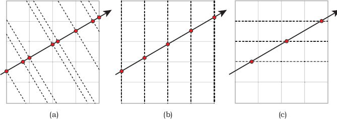
The following is a short description of what a regular grid is and how it works. A regular grid has the shape of an axis-aligned box that contains a group of objects. Figure 22.1(a) illustrates the idea in 2D. The box is subdivided into a number of cells that also have the shape of an axis-aligned box and are all the same size. Essentially, a regular grid is a spatial subdivision scheme that divides part of world space into a regular 3D cellular structure, hence the name. Roughly speaking, each cell stores a list of the objects that are in it, or partly in it, or may be in it.
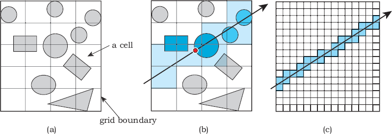
(a) 2D grid with objects, boundary, and cells; (b) a ray that passes through the grid hits the large dark sphere, as indicated by the red dot; (c) with a finer grid structure, the savings are more evident.
A ray that hits the grid only passes through certain cells, (shown shaded in Figure 22.1(b)), and is only intersected with the objects in these cells. This can save a lot of time, particularly when there are a large number of objects in the grid, as the ray will only be intersected with a small fraction of the objects. The situation is, however, better than that. The cells are tested strictly in the order that the ray traverses them as t increases. This means, roughly speaking again, that the first object that the ray hits is the nearest one, and the process then stops for that ray. This is the large sphere in Figure 22.1(b). The savings are better illustrated when there are more cells, as in Figure 22.1(c), and, of course, the savings are even higher in 3D.
For a scene with a large number n of objects, a grid will have cells in each direction, and rays will therefore be intersected with objects. That’s the worst-case scenario, however, where the rays traverse the whole grid. For densely packed objects such as the spheres in Section 22.4.3, where the rays don’t penetrate far into the grid, the number of objects intersected can be closer to O(log n) (see Table 22.2). The same situation applies to the hierarchical grids in Section 23.5. These types of asymptotic time complexities are a unique advantage that ray tracing has over algorithms whose render times are always proportional to n.
22.2 Construction
To construct a grid, we have to perform the following three tasks:
- add the objects;
- compute the bounding box;
- set up the cells.
Grids are geometric objects so that they can be intersected like any other object; they can also be nested—an important modeling characteristic. They also inherit from Compound, for two reasons. First, grids are compound objects because they consist of more than one component. Second, when we add objects to a grid, we need a temporary place to store them before we set up the cells; the Compound::objects data structure is convenient for this and simplifies the grid implementation. For example, it has code for assigning the same material to each object in the grid. Listing 22.1 shows a simplified declaration of the class.1
Adding an object to a grid is simple, as the following example shows. If we have the statement
Grid* grid_ptr = new Grid;
class Grid: public Compound {
public:
Grid(void);
// other constructors, etc.
virtual BBox
get_bounding_box(void);
void
setup_cells(void);
virtual bool
hit(Ray& ray, float& tmin, Shading& s);
virtual bool
shadow_hit(Ray& ray, float& tmin);
private:
vector<GeometricObject*> cells; // cells are stored in a 1D array
BBox bbox; // bounding box
int nx, ny, nz; // number of cells in the x-, y-, and z-directions
Point3D // compute minimum grid coordinates
min_coordinates(void);
Point3D // compute maximum grid coordinates
max_coordinates(void);
};
Listing 22.1. Declaration of the class Grid.
in a build function and have constructed a sphere called sphere_ptr, we use the statement
grid_ptr->add_object(sphere_ptr);
Here, add_object is inherited from Compound and adds the sphere pointer to the Compound::objects array.
To help illustrate how we compute the grid’s bounding box, Figure 22.2(a) shows the objects from Figure 22.1 with their bounding boxes. The grid’s bounding box is the union of the bounding boxes of the objects, as Figure 22.2(b) illustrates. This also defines the grid’s dimensions in the x-, y-, and z-directions because of its axis-aligned box shape.
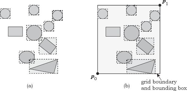
(a) Objects to be placed in a grid with their bounding boxes; (b) the grid’s bounding box.
The code for computing p0 and p1 is simple and is in the functions min_coordinates and max_coordinates, which are called from the setup_cells function. These points do not have to be stored in the grid. Listing 22.2 shows the code for get_min_coordinates, where kEpsilon is subtracted from the coordinates to make the grid slightly larger than the union of the objects’ bounding boxes. The function get_max_coordinates is analogous (see Question 22.6).
The next step is to divide the grid into the cells, which should be as cubical in shape as possible for intersection efficiency. We also have to consider how many cells to use. Although the cells are critical to the operation of the grid, they don’t need to be constructed or stored as separate objects. Instead, I’ll simulate them by indexing the 1D array of object pointers called cells in Listing 22.1.
Let nx, ny, and nz be the number of cells in the xw-, yw-, and zw- directions, respectively, let wx, wy, and wz be the dimensions of the grid, and let n be the number of objects to be placed in the grid. The following expressions, which are similar to those in Shirley (2000), can be used to calculate nx, ny, and nz so that the cells are roughly cubical:
Point3D
Grid::min_coordinates(void) {
BBox bbox;
Point3D p0(kHugeValue);
int num_objects = objects.size();
for (int j = 0; j < num_objects; j++) {
bbox = objects[j]->get_bounding_box();
if (bbox.x0 < p0.x)
p0.x = bbox.x0;
if (bbox.y0 < p0.y)
p0.y = bbox.y0;
if (bbox.z0 < p0.z)
p0.z = bbox.z0;
}
p0.x -= kEpsilon; p0.y -= kEpsilon;, p0.z -= kEpsilon;
return (p0);
}
Listing 22.2. The function Grid::min_coordinates.
Here, m is a multiplying factor that allows us to vary the number of cells. The + 1 in the formulae guarantees that the number of cells in any direction is never zero. From Equations (22.1), the total number of cells nxnynz is approximately m3n, provided nx >> 1, ny >> 1, and nz >> 1, which is usually the case. When m = 1, the number of cells is approximately equal to the number of objects, but that’s usually not the best value to use. If we have too many cells, the ray tracer wastes time testing for object intersections in empty cells, but if there are too few cells, it intersects too many objects. In the limit of a single cell (nx = ny = nz = 1), we essentially don’t have a grid, and there is no speed-up. Grids seem to have a sweet spot when there are about 8–10 times more cells than objects, because that’s when they are most efficient. By default, I use a factor of 8, which corresponds to m = 2. You should experiment with different values of m and compare the render speeds (see Exercises 22.5 and 22.6). The expressions (22.1) are easily translated into code, as Listing 22.4 shows.
Now to the indexing. According to Listing 22.1, the cells are represented by
which is a 1D array of length nx ny nz. The index of the (ix, iy, iz) cell is
which is the standard way that C and C++ programs store “3D” data structures in 1D arrays.
I place the objects into the cells by storing, for each cell, a “list” of all objects whose bounding boxes overlap the cell. The list will be empty if no bounding boxes overlap a cell, but the fact that the bounding box of an object overlaps a cell doesn’t mean that any part of the object is inside the cell. Figure 22.3(a) illustrates some of the possibilities for five objects and nine cells.
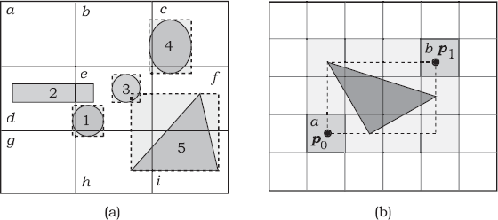
Table 22.1 lists the cells and their contents. Notice how objects 1, 2, 4, and 5 are in more than one cell.
The cells in Figure 22.3(a) and their contents.
Cell |
Objects |
|---|---|
a |
empty |
b |
4 |
c |
4 |
d |
1 and 2 |
e |
1, 2, 3, 4, 5, but only 1, 2, and 3 are actually in the cell |
f |
4 and 5 |
g |
1, but object 1 is not in the cell |
h |
1 and 5 |
i |
5 |
To discover which cells an object must be added to, we first compute the cells that contain the minimum and maximum corners of the object’s bounding box. Figure 22.3(b) illustrates this for a triangle, where p0 and p1 are in the cells labeled a and b, respectively. We need to compute which grid cell a given point p in world coordinates lies in. The cells are indexed with integers in the ranges (ix, iy, i) ∊ [0, n− 1] × [0, n− 1] × [0, n− 1]. Figure 22.4 shows a grid with four cells in the x-direction indexed with ix ∊ [0, 3], where p0 and p1 are the opposite corners of the grid. This figure also shows the distance px − p0x between p and p0 in the x-direction and the grid extent p1x - p0x in the x-direction.

A grid with four cells in the x-direction and a point p for which we wish to calculate the x cell index.
If we compute the ratio of these distances, multiply it by nx, and truncate the result to an integer, we almost have what we need:
For nx = 4, this produces the integer-valued step function in Figure 22.5(a).
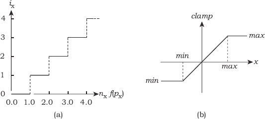
(a) The graph of ix from Equation (22.4) for nx = 4; (b) the graph of the clamp function from Listing 22.3.
The problem is that the point p can, and will, be located on any face of the grid’s bounding box. The negative face, where px = p0x, isn’t a problem because small negative values of the right-hand side resulting from round-off errors are truncated to zero. The problem lies with the positive face where px = p1x. Here, values of the right-hand side that are ≥ 1.0 return nx, which is out of range. We could fix this by adding an if statement
Listing 22.3. The clamp function.
but it can be fixed more generally by using the clamp function in Listing 22.3. This clamps the first parameter between the last two parameters, using linear interpolation to join the minimum and maximum values. Its graph is in Figure 22.5(b). As this is a utility function, it is in the file Maths.h.
I call clamp six times with max = nx − 1 to insert each object in the grid, truncating its output to an integer (see Listing 22.4).
The final construction step is to add each object to the cells that its bounding box overlaps. Figure 22.3(b) illustrates this in 2D for a triangle, where the bounding rectangle overlaps the light gray cells. The representation (22.2) of storing an object pointer in each cell is not the only representation that we can use. Exercise 22.7 covers two alternatives. I use (22.2) because it has a small memory footprint and runs the fastest on my computer. It does, however, have the most complicated code for inserting the objects into the cells because each cell will need to have one of the following types of information stored in it:
- the null pointer if there are no objects;
- an object pointer if there is one object;
- a compound-object pointer if there is more than one object.
As a result, the code needs to keep track of how many objects are in each cell, for which I use a temporary array. Listing 22.4 shows the function Grid:: setup_cells. This function is called from each build function that constructs a grid but only after all of the objects have been added to the grid. Listing 22.8 is an example of a build function that does this.
void
Grid::setup_cells(void) {
// find the minimum and maximum coordinates of the grid
Point3D p0 = min_coordinates();
Point3D p1 = max_coordinates();
// store them in the bounding box
bbox.x0 = p0.x; bbox.y0 = p0.y; bbox.z0 = p0.z;
bbox.x1 = p1.x; bbox.y1 = p1.y; bbox.z1 = p1.z;
// compute the number of cells in the x-, y-, and z-directions
int num_objects = objects.size();
float wx = p1.x - p0.x; // grid extent in x-direction
float wy = p1.y - p0.y; // grid extent in y-direction
float wz = p1.z - p0.z; // grid extent in z-direction
float multiplier = 2.0; // about 8 times more cells than objects
float s = pow(wx * wy * wz / num_objects, 0.3333333);
nx = multiplier * wx / s + 1;
ny = multiplier * wy / s + 1;
nz = multiplier * wz / s + 1;
// set up the array of cells with null pointers
int num_cells = nx * ny * nz;
cells.reserve(num_objects);
for (int j = 0; j < num_cells; j++)
cells.push_back(NULL);
// set up a temporary array to hold the number of objects stored in each cell
vector<int> counts;
counts.reserve(num_cells);
for (int j = 0; j < num_cells; j++)
counts.push_back(0);
// put objects into the cells
BBox obj_bbox; // object’s bounding box
int index; // cells array index
for (int j = 0; j < num_objects; j++) {
obj_bbox = objects[j]->get_bounding_box();
// compute the cell indices for the corners of the bounding box of the
// object
int ixmin = clamp((obj_bbox.x0 - p0.x) * nx / (p1.x - p0.x), 0, nx - 1);
int iymin = clamp((obj_bbox.y0 - p0.y) * ny / (p1.y - p0.y), 0, ny - 1);
int izmin = clamp((obj_bbox.z0 - p0.z) * nz / (p1.z - p0.z), 0, nz - 1);
int ixmax = clamp((obj_bbox.x1 - p0.x) * nx / (p1.x - p0.x), 0, nx - 1);
int iymax = clamp((obj_bbox.y1 - p0.y) * ny / (p1.y - p0.y), 0, ny - 1);
int izmax = clamp((obj_bbox.z1 - p0.z) * nz / (p1.z - p0.z), 0, nz - 1);
// add the object to the cells
for (int iz = izmin; iz <= izmax; iz++ // cells in z direction
for (int iy = iymin; iy <= iymax; iy++) // cells in y direction
for (int ix = ixmin; ix <= ixmax; ix++) { // cells in x
// direction
index = ix + nx * iy + nx * ny * iz;
if (counts[index] == 0) {
cells[index] = objects[j];
counts[index] += 1; index = 1
}
else {
if (counts[index] == 1) {
// construct a compound object
Compound* compound_ptr = new Compound;
// add the object already in cell
compound_ptr->add_object(cells[index]);
// add the new object
compound_ptr->add_object(objects[j]);
// store compound in current cell
cells[index] = compound_ptr;
// index = 2
counts[index] += 1;
}
else { // counts[index] > 1
// just add current object
cells[index]->add_object(objects[j]);
// for statistics only
counts[index] += 1;
}
}
}
}
// erase Compound::Objects, but don’t delete the objects
objects.erase (objects.begin(), objects.end());
// code for statistics on cell objects counts can go in here
// erase the temporary counts vector
counts.erase (counts.begin(), counts.end());
}
Listing 22.4. Code for storing objects in cells.
22.3 Traversal
As the grid has a long hit function, it’s worthwhile looking at this in stages. The following is top-level pseudocode.
if the ray misses the grid’s bounding box
return false
if the ray starts inside the grid
find the cell that contains the ray origin
else
find the cell where the ray hits the grid from the
outside
traverse the grid
Testing the ray for intersection with the bounding box at the start of the hit function isn’t just an efficiency measure. The minimum and maximum t values in the x-, y-, and z-directions that are computed in the process are used in the subsequent traversal code. This prevents us from just calling the bounding-box hit function in Listing 19.1, as it doesn’t return these values.
The hit function must be able to handle rays that start inside or outside the grid. Even with ray casting, we can put the camera inside the grid, and all the primary rays will then start inside. Shadow rays with any type of ray tracing also start inside the grid when we shade the objects in the grid. Finding the cell from which to start the traversal process is a simple application of the clamp function, as the code in Listing 22.5 shows. This is taken from the hit function, where ox, oy, and oz are the ray-origin coordinates, x0, y0 ... z1 are
int ix, iy, iz;
if (bbox.inside(ray.o)) {
ix = clamp((ox - x0) * nx / (x1 - x0), 0, nx - 1);
iy = clamp((oy - y0) * ny / (y1 - y0), 0, ny - 1);
iz = clamp((oz - z0) * nz / (z1 - z0), 0, nz - 1);
}
else {
Point3D p = ray.o + t0 * ray.d;
ix = clamp((p.x - x0) * nx / (x1 - x0), 0, nx - 1);
iy = clamp((p.y - y0) * ny / (y1 - y0), 0, ny - 1);
iz = clamp((p.z - z0) * nz / (z1 - z0), 0, nz - 1);
}
Listing 22.5. Code fragment from Grid::hit.
the grid’s bounding-box vertices, and t0 is the t value where the ray hits the bounding box.
The following is an example of how the ray can traverse the grid after hitting it from the outside. Figure 22.6(a) shows a ray that hits the cell labeled a. We test if the ray hits any objects in this cell, but since it’s empty, we proceed to test the other cells that the ray passes through, in the order of increasing t. The next two are the cells b and c. This process of stepping the ray through the grid is analogous to Bresenham’s classic algorithm for scan-converting lines (Bresenham, 1965, see also Foley et al., 1995). In this context, the technique is known as a 3D digital differential analyzer (3DDDA) and was developed by Fujimoto et al. (1986). In Figure 22.6(a), the ray is tested for intersection with the box 1 in cell b, which it misses, and then again in cell c, which it misses again. The ray is also tested with the sphere 2 in cell c, which it hits.

That is the end of the process as far as this ray is concerned; by construction, the hit point on object 2 is the closest hit point of all objects along the ray.
Although the ray passes through objects 3 and 4, these are not tested for intersection because of the intersection with the sphere 2. The other objects in the grid are also not tested (see Figure 22.6(b)).
To step a ray through the grid, we use the following astute observation by Amanatides and Woo (1987). Even though the intersections of the ray with the cell faces are unequally spaced along the ray, as indicated in Figure 22.7(a), the intersections in the x-, y-, and z-directions are equally spaced, as Figure 22.7(b) and (c) demonstrate. This simplifies the code, because it allows us to compute the ray parameter increments across the cells in the x-, y-, and z-directions. For a single cell, these are
Intersections with the cell boundaries are equally spaced in the x-, y-, and z-directions.
To simplify the following discussion, I’ll consider a ray traveling in the positive x- and y-directions in a 2D grid. For each cell, we have to work out if the next cell that the ray passes through is one across in the x-direction or one up in the y-direction. Figure 22.8 illustrates two configurations where the current cell is dark-shaded and the ray has entered it on an x (vertical) face. It could alternatively enter on a y face and have any positive gradient.
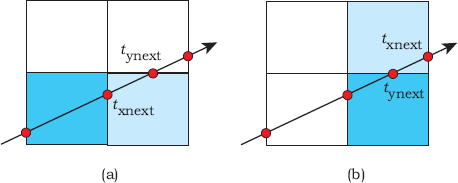
If t0 is the ray parameter where the ray enters the current cell, we compute txnext, the t value where it hits the next x face, and tynext, where it hits the next y face. If txnext < tynext, we go across, as in Figure 22.8(a); otherwise, we go up, as in Figure 22.8(b). To incorporate this into a working algorithm, we have to do the following:
- compute txnext and tynext for the initial cell;
- specify a condition to terminate the algorithm;
- step the ray though the grid.
Listing 22.6 is the code for Steps 1 and 2 (in 3D), where the initial cell coordinates ix, iy and iz have been computed by the code in Listing 22.5. The
float dtx = (tx_max - tx_min) / nx;
float dty = (ty_max - ty_min) / ny;
float dtz = (tz_max - tz_min) / nz;
float tx_next, ty_next, tz_next;
int ix_step, iy_step, iz_step;
int ix_stop, iy_stop, iz_stop;
tx_next = tx_min + (ix + 1) * dtx;
ix_step = +1;
ix_stop = nx;
ty_next = ty_min + (iy + 1) * dty;
iy_step = +1;
iy_stop = ny;
tz_next = tz_min + (iz + 1) * dtz;
iz_step = +1;
iz_stop = nz;
Listing 22.6. Set-up code for grid traversal.
while (true) {
GeometricObject* object_ptr = cells[ix + nx * iy + nx * ny * iz];
if (tx_next < ty_next && tx_next < tz_next) {
if (object_ptr && object_ptr->hit(ray, t, sr) && t < tx_next) {
material_ptr = object_ptr->get_material();
return (true);
}
tx_next += dtx;
ix += ix_step;
if (ix == ix_stop)
return (false);
}
else {
if (ty_next < tz_next) {
if (object_ptr && object_ptr->hit(ray, t, sr) && t <
ty_next) {
material_ptr = object_ptr->get_material();
return (true);
}
ty_next += dty;
iy += iy_step;
if (iy == iy_stop)
return (false);
}
else {
if (object_ptr && object_ptr->hit(ray, t, sr) && t < tz_
next) {
material_ptr = object_ptr->get_material();
return (true);
}
tz_next += dtz;
iz += iz_step;
if (iz == iz_stop)
return (false);
}
}
}
Listing 22.7. Grid traversal in 3D.
variables ix_stop, iy_stop, and iz_stop will tell the algorithm when the ray is about to exit the grid.
Listing 22.7 shows how the grid is traversed in 3D. If the cell is empty, the object pointer will be null, which has to be checked before the hit function is called. Because of the lazy evaluation of the && operator in C++, the hit function will only be called when there is an object present. Note that a hit is only recorded when a hit occurs for t < txnext or t < tynext, to confine any hits to the current cell.
The full hit function is on the book’s website as part of the Grid class.
22.4 Testing
Grids are complex objects that you need to test thoroughly. This section contains some tips for doing this and some test scenes.
22.4.1 Testing Tips
Turn the grid off. Unless you are rendering huge numbers of objects, you can always render test scenes with and without using the grid and compare the results. If the grid is working correctly, the results must be identical. This technique is applicable to all rendering situations. It’s usually not much work to change the build functions. To use the grid, you add objects to the grid as they are constructed and then add the grid to the world. To turn the grid off, you add the objects to the world but don’t add the grid to the world.
Use all types of rays. Test the grid with primary, secondary, and shadow rays that start inside and outside the grid. This will involve you placing the camera inside the grid and, in later chapters, using reflective and transparent materials.2
Use special configurations. Grids will sometimes work correctly when rays travel at arbitrary angles to the coordinate axes but fail when they are parallel to the axes or the coordinate planes. The reason is that in this case, the grid hit function divides by zero. Use tests where rays have these orientations. You should also test a grid that’s centered on the world axis and has axis-aligned objects.
Use a single object. Test the grid with a single object, for example, a sphere centered on the origin, an axis-aligned cube centered on the origin, and an axis-aligned cube with one vertex at the origin. The cube in this last example has three of its faces in coordinate planes. Place the camera inside the cube. Use a single cell and multiple cells. Also, test the grid by looking along the world coordinate axes.
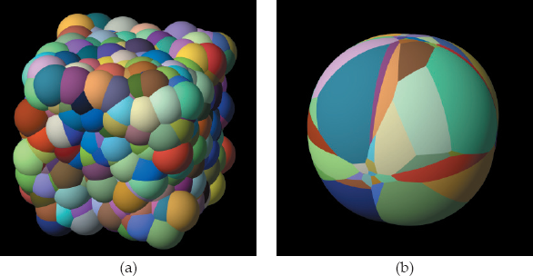
22.4.2 Eight Boxes
Figure 22.9(a) shows a grid with eight axis-aligned boxes. Although this is a simple scene, it’s a tough test because of the symmetries involved and the axis alignment of the objects and the lights. Figure 22.9(b) shows a vertical cross section through the four “front” boxes in Figure 22.9(a).

(a) Orthographic view of eight boxes in a grid; (b) vertical cross section of the grid, showing its bounding box and cells.
The boxes are arranged so that the grid’s bounding box is a cube centered on the origin with one box at each corner. Each box therefore has three faces in the bounding-box faces. There are four cells in each direction, as indicated by the dashed lines in Figure 22.9(b), and the size of the bottom four boxes is such that their three faces inside the grid lie on cell faces. The scene is illuminated by six directional lights in the ±x-, ±y-, and ±z-directions, so that the shadow rays, which all start inside the grid or on its boundary, travel parallel to the coordinate axes in both directions.
The only way to get all of the primary rays parallel to a coordinate axis is to use an orthographic camera. Figure 22.10(a) is an orthographic view looking down the y-axis where the eye point is at the origin. This places all of the ray origins in the (x, z) plane and on cell faces. Only the bottom four boxes are visible, but the shadow rays still intersect the other boxes.

(a) Orthographic view of the cubes looking down the y-axis; (b) spherical panoramic view from the center of the grid.
Figure 22.10(b) shows a 360°× 180° spherical panoramic view from inside the grid where the eye point is at the origin. As such, it’s at a corner of 8 cells. The view direction is along the negative x-axis. This demonstrates that shadows are working for the three lights coming from the negative coordinate axis directions (see Question 22.4).
22.4.3 Random Spheres
If your grid can correctly render the boxes in Section 22.4.2, it’s probably in good shape, but that scene doesn’t have enough objects to demonstrate the speed advantages of grids. Random spheres in a cube are a simple way to do this, as indicated in Listing 22.8. Here, the spheres are randomly placed in a cube that’s centered on the origin, their radii are scaled according to the number of spheres, and their colors are random.3
Some results are shown in Figure 22.11, where Figure 22.11(a)–(d) were rendered with a pinhole camera on the z-axis with one ray per pixel, a single directional light, and no shadows. The million-spheres grid used about 250 MB of RAM on my computer, but you could save memory by letting the spheres
void
World::build(void) {
// construct viewplane, integrator, camera, and lights
int num_spheres = 100000;
float volume = 0.1 / num_spheres;
float radius = pow(0.75 * volume / 3.14159, 0.333333);
Grid* grid_ptr = new Grid;
set_rand_seed(15);
for (int j = 0; j < num_spheres; j++) {
Matte* matte_ptr = new Matte;
matte_ptr->set_ka(0.25);
matte_ptr->set_kd(0.75);
matte_ptr->set_cd(randf(), randf(), randf());
Sphere* sphere_ptr = new Sphere;
sphere_ptr->set_radius(radius);
sphere_ptr->set_center( 1.0 - 2.0 * rand_float(),
1.0 - 2.0 * rand_float(),
1.0 - 2.0 * rand_float());
sphere_ptr->set_material(matte_ptr);
grid_ptr->add_object(sphere_ptr);
}
grid_ptr->setup_cells(); // must be called after all the
// spheres have been added
add_object(grid_ptr);
}
Listing 22.8. Partial build function for a grid of random spheres.
share a common material. Figure 22.11(e) is a three-faced view of 100,000 spheres with shadows.

Face-on views of a cube of random spheres with 1000 (a), 10,000 (b), 100,000 (c), and one million (d) spheres; (e) three-faced view of 100,000 spheres with shadows.
Table 22.2 compares the render times for the face-on views using the grid and using exhaustive ray tracing. All images were rendered at a resolution of 400 × 400 pixels on a 450 MHz G3 Macintosh with 512 MB RAM. The table also shows the speed-up factors, which increase as the number of spheres increases. The speed-up for one million spheres is estimated using linear extrapolation. A value of m = 2 in Equation (22.1) was used, which results in eight times more cells than objects.
Render times for random spheres in a cube.
Number of Spheres |
Render Times in Seconds |
Grid Speed-Up Factors |
|
|---|---|---|---|
With Grid |
Exhaustive |
||
10 |
1.5 |
2.5 |
1.6 |
100 |
2.0 |
16 |
8 |
1000 |
2.7 |
164 |
61 |
10,000 |
3.8 |
2041 |
537 |
100,000 |
4.7 |
22169 (6 hours) |
4717 |
1,000,000 |
5.2 |
forget it! |
≈ 46,307 |
The figure on the first page of this chapter is a perspective view of 1000 spheres with the camera inside the grid. Note the extreme perspective distortion.
22.4.4 Some Issues
A random cube of spheres is ideal for the grid structure, particularly when there are large numbers of spheres uniformly distributed in the cube. The fact that the rays don’t penetrate the grid very far before they hit a sphere also contributes to the low rendering times. This is demonstrated by the fact that render times for 100,000 and one million spheres are not much different. The triangle meshes in Chapter 23 provide more realistic tests for the grid.
As discussed in Chapter 1, I use doubles for the Sphere, Vector3D, and Point3D data members and for the object-intersection calculations. I couldn’t render more than about 10,000 of these spheres with floats, due to numerical-precision problems; the spheres were just too small. My students who use PCs don’t have this problem.
22.5 Grids and Transformed Objects
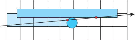
For modeling and rendering flexibility, we must be able to include transformed objects in grids. To do this, we need the axis-aligned bounding boxes of the transformed objects, as Figure 22.12 illustrates for a transformed sphere.

Unfortunately, it’s difficult to compute the axis-aligned bounding box of an arbitrary object that has been subject to an arbitrary sequence of transformations. It’s even difficult for the transformed object in Figure 22.12, which is just a rotated ellipsoid.
In practice, we have to settle for second best, which is the axis-aligned bounding box of the original object’s transformed bounding box. Did you get that? Don’t worry; Figure 22.13 illustrates what I’m talking about. For example, let’s scale the sphere on the left to produce an ellipsoid and its bounding box defined by p′0 and p′1. Now rotate this and the bounding box to produce the rotated ellipsoid and rotated bounding box p′′0 and p′′1 on the right. This bounding box is the tightest fit to the ellipsoid, but because it’s no longer axis-aligned, we can’t use it. We also can’t easily compute the axis-aligned bounding box of the rotated ellipsoid, indicated by the green rectangle. So, what can we do? We can compute the axis-aligned bounding box of the rotated bounding box, as defined by p′′′0 and p′′′1 and as indicated by the gray rectangle. As you can see, it’s larger than the axis-aligned bounding box of the rotated object, with the result that the transformed object will be placed in more grid cells than necessary. But this just affects the efficiency of the grid; the results will still be correct, of course. Axis-aligned boxes computed this way are oft en loose fits to the objects, particularly when scaling or shearing is combined with rotation, but it’s the best we can do.

The axis-aligned bounding box of the rotated bounding box is larger than the axis-aligned bounding box of the rotated object.
Because the rotated vertices p″0 and p″1 in Figure 22.13 don’t define the extremities of the axis-aligned box of the rotated bounding box, we need to transform all eight vertices of the original object’s bounding box and use these transformed vertices to work out the minimum and maximum vertices p′″0 and p′″1. The catch is that we need to use the forward transformations, not their inverses. The instance objects thus need access to the transformation matrix as well as its inverse. Fortunately, we only need the bounding boxes during grid construction; they are not used to ray trace the transformed objects. The transformation matrix, which I’ve called forward_matrix, can therefore be static in the Instance class. We must, however, store the bounding box with each instance because it has to be accessed three times during the grid construction. It’s used twice to compute the grid’s dimensions and once to place the transformed objects in the grid.4 The revised declaration of the Instance class appears in Listing 22.9, where the new member functions and data members are in blue.
class Instance: public GeometricObject {
public:
// constructors, etc.
void
compute_bounding_box(void);
virtual BBox
get_bounding_box (void);
virtual bool
shadow_hitt(const Ray& ray, float& tmin) const;
virtual bool
hit(const Ray& ray, float& tmin, ShadeRec& sr) const;
void
translate(const float dx, const float dy, const float dz);
// other transformation functions
private:
GeometricObject* object_ptr; // object to be transformed
Matrix inv_matrix; // inverse transformation matrix
bool transform_texture; // do we transform textures?
static Matrix forward_matrix; // transformation matrix
BBox bbox; // bounding box
};
Listing 22.9. New declaration of the class Instance.
The forward_matrix data member needs to be initialized to the unit matrix at the start of the Instance.cpp file with the code
The transformation matrix must be built up at the same time as the inverse matrix is built up. Listing 22.10 illustrates how to do this with the Instance:: translate function, where I’ve added the forward_matrix code to the function in Listing 21.8. Note that the translation matrix is pre-multiplied in accordance with Equation (20.10). The other transformation functions will need similar code added.
The last thing to do when constructing an instance is to call the function Instance::compute_bounding_box. If you want to store a transformed object in a grid, you must call this function in the build function. I haven’t reproduced the code for this function here because it’s lengthy and not particularly interesting, except for one point. After it has finished with the transformation matrix, it must set it back to the identity matrix, ready for the next instance. Remember: there is only one copy of a static variable.
Figure 22.14 shows a spherical panoramic view of a grid that contains 25 random spheres that were constructed by scaling and translating generic spheres.

void
Instance::translate(const float dx, const float dy, const float dz) {
Matrix inv_translation_matrix; // temporary inverse translation matrix
Matrix translation_matrix; // temporary translation matrix
inv_translation_matrix.m[0][3] = -dx;
inv_translation_matrix.m[1][3] = -dy;
inv_translation_matrix.m[2][3] = -dz;
inv_matrix = inv_matrix * inv_translation_matrix; // post-multiply
translation_matrix.m[0][3] = dx;
translation_matrix.m[1][3] = dy;
translation_matrix.m[2][3] = dz;
forward_matrix = translation_matrix * forward_matrix; // pre-multiply
}
Listing 22.10. The function Instance::translate with the forward_matrix code included.
The lines on their surfaces, which are textures, help to illustrate the distortions produced by the panoramic camera. All of the spheres are the same size.
The bunnies in Figure 21.4 are stored in a grid after being translated. Because each bunny is also a grid, this figure illustrates nested grids. You should be able to reproduce this after you have finished Chapter 23.
22.6 Comparison with BVHs
Bounding volume hierarchies are more adaptive to the scene geometry than grids because the cell sizes and locations are determined by the objects. They can therefore be more efficient for scenes where the objects are unevenly distributed in space, such as triangle meshes. They have a much simpler, recursively defined hit function than the grid. Their construction is not as straightforward as the grid’s because they require a cost-function heuristic for optimal performance. The analogous cost function for grids is the number of cells per object. Compared to a grid, it’s more trouble to handle rays that start inside a BVH, because these rays can start arbitrarily deep in the hierarchy.
Further Reading
Most of the fundamental breakthroughs in ray-tracing acceleration occurred during the 1980s. The reason is that ray tracing was so slow on the machines of the time that people started to think about how to make it run faster, right from the start. The following are some of the significant contributions.
The earliest papers on acceleration, by Rubin and Whitted (1980) and Weghorst et al. (1984), used bounding volume hierarchies. The first spatial subdivision algorithms were by Glassner (1984), who used octrees, and Kaplan (1985), who used kd-trees. The regular grid and its 3DDDA traversal algorithm originated with Fujimoto et al. (1986). Goldsmith and Salmon (1987) described an algorithm for automatically generating bounding volume hierarchies because the hierarchies of the time were either built by hand or were just based on the scene data structure. They were therefore less than optimal in terms of performance. Kirk and Arvo (1988) provide an excellent survey of acceleration techniques as they existed in 1988. Samet (1990a, 1990b) and Langetepe and Zachmann (2006) are books on spatial data structures.
My discussion of regular grids is based on Shirley (2000), who recommended that each cell store an object pointer and presented pseudocode for the hit function. Some aspects of the regular grid are also presented in Shirley et al. (2005).
Shirley and Morley (2003) has the complete code for a bounding volume hierarchy. Pharr and Humphreys (2004) discusses regular grids and kd-trees.
Questions
- 22.1. Figure 22.15 is similar to Figure 22.6, but here, the ray hits the box behind the sphere. Would this situation cause problems for the grid hit function? Consider the cells that the ray traverses before it gets to the sphere. In each of these cells the ray will be tested against the box, whose hit function will return true.
- 22.2. One of the geometric objects can’t be stored in a grid. Which one is it, and what is the reason?
- 22.3. There are certain shadows visible in Figure 22.10(a). In which directions do the shadow rays travel that created these?
- 22.4. How can you tell from Figure 22.10(b) that shadows are working correctly for the directional lights in the negative x-, y-, and z-directions?
- 22.5. Which transformations leave the transformed bounding box axis-aligned?
- 22.6. Consider a scene that consists of a grid that contains a single axis-aligned box with a brown matte material, a pinhole camera and a point light inside the box, and the Uffizi image on a large surrounding sphere. The scene will be rendered with ray casting. Figure 22.16(a) shows the inside of the box illuminated by the point light. Definitely not an interesting image. Figure 22.16(b) is the same scene rendered without the grid’s bounding box being expanded with kEpsilon in the functions get_min_ coordinates and get_max_coordinates. In this case, the grid is exactly the same size as the axis-aligned box’s bounding box. Can you explain this noisy image of the Uffizi buildings?

Exercises
- 22.1. Implement the Grid class on the book’s website and use the scenes in Section 22.4 to test it.
- 22.2. Section 22.4 only covered a few of the many tests that you should perform on the boxes grid. Here are a few more suggestions. Use the orthographic camera to look at the cubes from the positive and negative x-, y-, and z-directions. Also use it to look parallel to the coordinate planes where the primary rays aren’t parallel to a coordinate axis. Use the perspective camera with the eye point at various locations outside the grid, on the grid faces, and inside the grid.
- 22.3. Make the random spheres in Section 22.4.3 larger and see how this affects the build times, memory footprints, and rendering times. As an example, Figure 22.17(a) shows 1000 spheres that are 10 times larger than those in Figure 22.11(a), and in Figure 22.17(b), the spheres are 250 times larger.
- 22.4. In Figures 22.9 and 22.10, I hard-wired nx = ny = nz = 4 into the Grid:: setup_cells function. Give the user the option to set a common value for these in the build functions.
- 22.5. My grid implementation hard-wires in the value m = 2. Give the user the option to set this in the build functions.
- 22.6. Experiment with various values of m in Equations (22.1) and compare the speeds.
- 22.7. Below are two alternative ways to represent the cells. Compare the build times, memory footprints, and rendering times with the representation (22.2).
vector<Compound*> cells;vector<vector<GeometricObject*> > cells;These will affect the function Grid::setup_cells, which will be simpler than the version in Listing 22.4, and will also affect the hit functions. In the Compound object representation, some of the objects will be empy (see Exercise 19.21).
- 22.8. Get a grid to cast shadows on another object. A good test would be either the boxes grid or the random spheres and some planes. Figure 22.18(a) is an example of the latter. Include a case where the plane cuts through the grid, as this would be another test for the grid’s regular hit function.
- 22.9. Figure 22.18(a) shows 25 random spheres in a grid, with three planes and shadows. In Figure 22.18(b), the spheres have been individually scaled by (a, b, c) = (1.0, 0.25, 1.0) before they have been added to the grid. In Figure 22.18(c), the grid has been scaled by the same amounts instead of the spheres. Although the spheres are the same shape in both images, the results are different. Can you explain this? It might help to render the images with the camera on the positive x- or z-axis. Reproduce these figures.
- 22.10. Check that nested instances work when you store them in a grid.
- 22.11. Implement a bounding volume hierarchy (BVH) acceleration scheme and compare its performance with the regular grid for a variety of scenes, including triangle meshes.

1. I’ll add other data members and member functions in Chapter 23 to handle triangle meshes.
2. The random box city figures in Chapter 11 were also rendered using a grid, and in Figure 11.12, the camera is inside the grid.
3. The code for generating the spheres in Listing 22.8 is by Peter Shirley.
4. You would only need to use the bounding box twice if you combined the min_coordinates and max_coordinates functions.