
Chapter 18
Area Lights

Objectives
By the end of this chapter, you should:
- understand how area lights are modeled and rendered;
- have implemented a number of area lights;
- have implemented an environment light.
All real light sources have finite area, and as such, their illumination and soft shadows can add great realism to your images. This is in contrast to the sharp-edged shadows that we get from point and directional lights. The price we have to pay is more sample points per pixel and longer rendering times, but the results are worth it.
I’ll discuss here a flexible lighting architecture that will allow you to use a variety of geometric objects as area-light sources. I’ll also discuss rectangular and environment lights. There’s a lot of work involved in this because it’s not just a matter of adding area lights to the existing light classes. We also have to add a new tracer to perform the Monte Carlo integration, add an emissive material, and make changes to the Material, GeometricObject, and Light base classes. If you want to skip this, at least on a first reading, but still want to render soft shadows, look at Exercises 18.1 and 18.2. These cover how to modify point and directional lights to produce good area-light shading effects for a few percent of the work compared to the full implementation.
Because a lot of fiddly programming details are required to implement area lights, most of the classes are on the book’s website.
18.1 Area-Lighting Architecture
One way to implement area lights is to have a separate class for each type of area light. While there’s nothing wrong with this approach, you would have to write each class, and a lot of the code would be repeated.
An alternate approach is to have a single area-light class that contains a pointer to a geometric object that provides the illumination through an emissive material. In this approach, the type of object automatically determines the type of light, and the illumination can be computed polymorphically. In principle, this allows any type of geometric object to be a light source, provided we can accurately estimate its incident radiance at a surface point p. I’ve adopted this approach.
We can use a number of techniques to compute the direct incident radiance. The first is where shadow rays are shot towards sample points on the light surface. Each type of object that’s used as an area light source must therefore be able to provide sample points on its surface and the normal at each point. How easy or difficult these tasks are depends on the object. For a planar object such as a rectangle, it’s simple to generate uniformly distributed samples on its surface, and the normal is the same at each point. For other objects, such as triangle meshes, the process can be more difficult. This is used with the area form of the rendering equation.
A second technique is where the shadow rays are shot into the solid angle subtended at p by the object and tested for intersection with the light object. This is used with the hemisphere form of the rendering equation, with an added visibility function.
A third technique is where the rays sample the BRDF at p instead of sampling the lights. With this technique, the rays don’t have to hit the light surface and don’t have to be shadow rays. They can be secondary rays that are traced recursively into the scene to estimate the direct or indirect illumination at p. This technique is used with the hemisphere form of the rendering equation.
Which technique is the most efficient depends on the BRDF at p and on the light source. The BRDF can vary from perfect diffuse reflection to perfect specular reflection, while the solid angle subtended by the light at p can vary from very small to the whole hemisphere above p. Figure 18.1 illustrates the case of a specular BRDF and a hemispherical light.
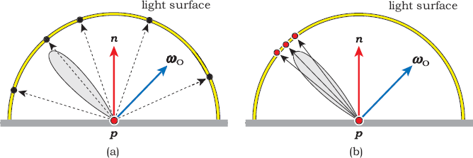
Specular BRDF and hemispherical light with ray directions determined by sample points on the light surface (a) and by sampling the BRDF (b).
In Figure 18.1(a), the shadow rays are directed to sample points on the light, but most of these are in directions where the BRDF is small. The result will be undersampling of the BRDF and noisy images. In Figure 18.1(b), the rays sample the BRDF, which in this case is more efficient because most of the rays are in directions where the BRDF is not small.
Figure 18.2 illustrates the opposite situation, where the BRDF is Lambertian and the light subtends a small solid angle at p. In this case, sampling the light surface, as illustrated in Figure 18.2(a), is more efficient than sampling the BRDF in Figure 18.2(b) because there, most of the rays miss the light.
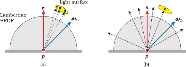
Lambertian BRDF and a small light with ray directions determined by sample points on the light surface (a) and by sampling the BRDF (b).
The general technique of choosing the most efficient sampling technique for a given light and BRDF is an example of importance sampling, as discussed in Section 13.11.
In this chapter, I’ll use the first technique to estimate the direct illumination from rectangular, disk, and spherical lights, with the area form of the rendering equation.1 I’ll also use the second technique to estimate the direct illumination from environment lights, with the hemisphere form of the rendering equation.
18.2 Direct Rendering
There are two aspects of shading with an area light. The first is rendering the light itself, which can be directly visible, unlike directional and point lights. The second is computing the light’s illumination on other objects in the scene. Figure 18.3 illustrates these two aspects, where each ray that hits an area light returns the emitted radiance Le.
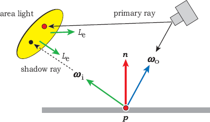
An area light can be directly visible as well as providing direct illumination to other objects in the scene.
The geometric object that acts as the area light is stored in the World:: objects array like any other object, so that it can be rendered without special treatment as far as primary and secondary rays are concerned. I attach an Emissive material to each such object, which provides the self-emissive term Le(p, ωo) in the rendering equation and its solution (13.29).
18.3 Estimating Direct Illumination
For direct illumination, the exitant radiance Lo(p′, − ωi) in the area form of the radiance equation (13.25) reduces to the emitted radiance at p′; that is, Lo(p′, − ωi) = Le(p′, − ωi). In addition, Le is only nonzero on light sources, a fact that allows us to reduce the integration domain from all surfaces in the scene to light-source surfaces only. That’s a major simplification. The reflected radiance at a surface point p can then be written as
where Alights is the set of all light surfaces, and dA′ is a differential surface element around p′. As a reminder, ωi in Equation (18.1) is given by Equation (13.27): ωi = (p′ − p)/||p′ − p||. If there are nl area lights in the scene, we can write Equation (18.1) as the following sum over them:
Consider a scene that contains a single area light, so that there’s a single term in the sum (18.2). The Monte Carlo estimator for the integral is
for ns sample points p′j, j = 1, ..., ns. Here, p(p′j) is the probability density function defined over the surface of the light.
The difficult part is defining the pdf, which can be nontrivial for lights that are not planar. Ideally, we want the pdf to match the contribution of each sample point to the estimator, but that’s usually not possible. The simplest choice is to use samples that are uniformly distributed over the light surface, in which case the pdf is just the inverse area of the light: p(p′j) = 1 / Al, for all p′j. This is particularly suitable for planar lights.
There are two major sources of noise in images generated by (18.3). For points p in the penumbra region of shadows, the visibility function V(p, p′j) will be zero for some sample points and nonzero for others, and therefore penumbrae are typically noisy, unless we use large numbers of samples. The 1/d2 term in the geometric factor G(p, p′j) can cause large variations in the estimator, and therefore noise, even for points receiving full illumination. This is particularly true for large lights that are close to the surfaces being shaded.
18.4 The Area-Lighting Tracer
Because the Monte Carlo estimator (18.3) involves G(p, p′j) and the pdf, we have to write new material-shade functions to evaluate this estimator and call these from a new tracer. The material functions are called area_light_shade, and the tracer is called AreaLighting, according to the notation established in Sections 14.5 and 14.7. Listing 18.1 shows the code for the function AreaLighting::trace_ray. Note that this only differs from RayCast:: trace_ray in Listing 14.10 by calling material_ptr->area_light_shade instead of material_ptr->shade.
18.5 The Emissive Material
The radiance in the outgoing direction ωo from a self-emitting material is the emitted radiance Le. In general, this can depend on location and direction, as indicated by the p and ωo arguments in Le(p, ωo), but to keep the discussion in this chapter as simple as possible, I’ll only consider spatially invariant, isotropic emissive materials, where Le is independent of p and ωo.2 I’ll also assume that emissive materials don’t reflect or transmit light so that when a primary or secondary ray hits a self-emissive object, no further rays are generated. With these assumptions, the Emissive material class is quite simple, as Listing 18.2 shows. In particular, there are no BRDFs involved because it doesn’t reflect light.
The emissive material stores a radiance scaling factor ls and an emitted color ce, in analogy to light sources. Notice that there is both a shade and an area_light_shade function. The shade function allows us to use the emissive material with other tracers such as RayCast and Whitted and thereby to render emissive objects in scenes without shading with them. Both functions return the emitted radiance Le = ls ce, but only when the incoming ray is on the same side of the object surface as the normal; otherwise, they return black. In other words, an object with an emissive material only emits light on one side of its surface. The constant emitted color and the isotropic emission result in emissive objects being rendered with a constant color.
Listing 18.3 shows the code for Emissive::area_light_shade, where the incoming ray is stored in sr in the function AreaLighting::trace_ray.
RGBColor
AreaLighting::trace_ray(const Ray ray, const int depth) const {
ShadeRec sr(world_ptr->hit_objects(ray));
if (sr.hit_an_object) {
sr.ray = ray;
return(sr.material_ptr->area_light_shade(sr));
else
return(world_ptr->background_color);
}
Listing 18.1. The function AreaLighting::trace_ray.
class Emissive: public Material {
private:
float ls; // radiance scaling factor
RGBColor ce; // color
public:
// constructors, set functions, etc.
void
scale_radiance(const float _ls);
void
set_ce(const float r, const float g, const float b);
virtual RGBColor
get_Le(ShadeRec& sr) const;
virtual RGBColor
shade(ShadeRec& sr);
virtual RGBColor
area_light_shade(ShadeRec& sr);
};
Listing 18.2. Code from the Emissive material class.
I should emphasize that this function is called from AreaLighting::trace_ray when the nearest hit point of a primary ray or secondary ray is on the surface of an area light, so that the normal stored in sr is the normal at the hit point. It’s therefore part of the direct rendering of the area light, not its direct illumination on other surfaces, which is handled by the AreaLight class.
RGBColor
Emissive::area_light_shade(ShadeRec& sr) {
if (-sr.normal * sr.ray.d > 0.0)
return (ls * ce);
else
return (black);
}
Listing 18.3. The function Emissive::area_light_shade.
RGBColor
Matte::area_light_shade(ShadeRec& sr) {
Vector3D wo = -sr.ray.d;
RGBColor L = ambient_brdf->rho(sr, wo) * sr.w.ambient_ptr->L(sr);
int num_lights = sr.w.lights.size();
for (int j = 0; j < num_lights; j++) {
Vector3D wi = sr.w.lights[j]->get_direction(sr);
float ndotwi = sr.normal * wi;
if (ndotwi > 0.0) {
bool in_shadow = false;
if (sr.w.lights[j]->casts_shadows()) {
Ray shadow_ray(sr.hit_point, wi);
in_shadow = sr.w.lights[j]->in_shadow(shadow_ray,
sr);
}
if (!in_shadow)
L += diffuse_brdf->f(sr, wo, wi) * sr.w.lights[j]->L(sr)
* sr.w.lights[j]->G(sr) * ndotwi /
sr.w.lights[j]->pdf(sr);
}
}
return (L);
}
Listing 18.4. The function Matte::area_light_shade.
The function Emissive::get_Le, which is called from the area light’s L function in Listing 18.10, also returns the emitted radiance lsce.
18.6 Other Materials
Since Emissive::get_Le is called polymorphically, it has to be added as a virtual function to the base Material class. It’s not pure virtual there as I’ve only defined it for the two materials Emissive and SV_Emissive.3 We must also add the function area_light_shade to the Material class, but it has to be defined for every material that we want to render with area-light shading. Listing 18.4 shows the function Matte::area_light_shade with shadows. In this context, the area light’s in_shadow function computes the visibility function V(p, p′j) in Equation (18.3). You can, of course, turn shadows on or off in the build functions. Notice that the light functions G and pdf are also called polymorphically. As a result, you will have to add these to the Light base class as virtual functions, where they can both return 1.0. This will allow you to add point and directional lights to scenes with area lights, as in Figure 18.9.
18.7 The Geometric Object Classes
A geometric object that’s also a light source must provide the following three services to the AreaLight class:
- sample points on its surface,
- the pdf at each sample point (which needs the area),
- the normal at each sample point.
To provide the samples, I store a pointer to a sampler object in the geometric object, but to save memory, I only do this with object types that are used for area lights: disks and rectangles, for the time being. We also have to compute the object’s inverse area, as the pdf will return this. It’s most efficient to compute area once when the object is constructed and to store the inverse area, as this saves a division each time the pdf function is called.
As an example, Listing 18.5 shows the class Rectangle with the new data members and member functions in blue. As the functions sample, pdf, and get_normal will be called polymorphically from AreaLight, they will have to be added as virtual functions to the GeometricObject base class.
class Rectangle:: public GeometricObject {
private:
Point3D p0;
Vector3D a;
Vector3D b;
Normal normal;
Sampler* sampler_ptr;
float inv_area;
public:
// constructors, access functions, hit functions
void
set_sampler(Sampler* sampler);
virtual Point3D
sample(void);
virtual float
pdf(ShadeRec& sr);
virtual Normal
get_normal(const Point3D& p);
};
Listing 18.5. The class Rectangle.
Point3D
Rectangle::sample(void) {
Point2D sample_point = sampler_ptr->sample_unit_square();
return (p0 + sample_point.x * a + sample_point.y * b);
}
Listing 18.6. The function Rectangle::sample.
The function sample uses the rectangle’s corner vertex p0 and the edge vectors a and b to generate sample points on the surface. The code is in Listing 18.6.
There is, however, a flaw in this code. Unless the rectangle is a square, the samples will not be uniformly distributed on its surface. The distribution will be stretched in the largest direction, or equivalently, squashed in the smallest direction. Although I’ll only use rectangular lights that are square in this chapter, you should test other shapes (see Exercise 18.9). There shouldn’t be a major problem unless the light has a skinny shape.
I won’t reproduce the functions pdf and get_normal, as these just return the inverse area and the specified normal, respectively.
18.8 The Area Light Class
With code for the other classes out of the way, we can now look at the AreaLight class, the declaration for which is in Listing 18.7.
class AreaLight: public Light {
public:
// constructors, access functions, etc.
virtual Vector3D
get_direction(ShadeRec& sr);
virtual bool
in_shadow(const Ray& ray, const ShadeRec& sr) const;
virtual RGBColor
L(ShadeRec& sr);
virtual float
G(const ShadeRec& sr) const;
virtual float
pdf(const ShadeRec& sr) const;
private:
GeometricObject* object_ptr;
Material* material_ptr; // an emissive material
Point3D sample_point; // sample point on the surface
Normal light_normal; // normal at sample point
Vector3D wi; // unit vector from hit point to sample point
};
Listing 18.7. The class AreaLight.
Vector3D
AreaLight::get_direction(ShadeRec& sr) {
sample_point = object_ptr->sample();
light_normal = object_ptr->get_normal(sample_point);
wi = sample_point - sr.hit_point;
wi.normalize();
return (wi);
}
Listing 18.8. The function AreaLight::get_direction.
The five member functions get_direction, in_shadow, L, G, and pdf are called in this order from Matte::area_light_shade, and so that’s the best order to present and discuss them. Because of the area-lighting architecture, where a lot of the work is done in other classes, these functions are all small and simple.
The function get_direction in Listing 18.8 does more than just return the unit direction ωi from the point being shaded to the sample point; it also stores the sample point, the normal at the sample point, and ωi in data members. The reason is that these are also required in the functions in_shadow, L, and G. Although it’s best for each function to perform a single task, the multitasking in this case is a matt er of practical necessity, as a given sample point can only be accessed once.
The geometric object’s get_normal function, called from AreaLight:: get_direction, will work for planar objects and objects that are defined by a single implicit function but will not work for other objects, for example, an axis-aligned box (see the Notes and Discussion section).
bool
AreaLight::in_shadow(const Ray& ray, const ShadeRec& sr) const {
float t;
int num_objects = sr.w.objects.size();
float ts = (sample_point - ray.o) * ray.d;
for (int j = 0; j < num_objects ; j++)
if (sr.w.objects[j]->shadow_hit(ray, t) && t < ts)
return(true);
return(false);
}
Listing 18.9. The function AreaLight::in_shadow.
RGBColor
AreaLight::L(ShadeRec& sr) {
float ndotd = -light_normal * wi;
if (ndotd > 0.0)
return (material_ptr->get_Le(sr));
else
return (black);
}
Listing 18.10. The function AreaLight::L.
The in_shadow function in Listing 18.9 tests if the shadow ray hits an object between the hit point and the sample point.
The function L in Listing 18.10 checks that the shadow ray hits the light surface on the same side as the normal before returning the material’s emitted radiance.
The function G in Listing 18.11 computes the cosine term cos θ′ = −n′j • ωi,j divided by d2. As such, it’s not the full geometric factor G(p, p′j), as the other cosine factor n • ωi,j is computed separately in Matte::area_light_shade.
The function pdf in Listing 18.12 simply calls the object’s pdf function.
float
AreaLight::G(const ShadeRec& sr) const {
float ndotd = -light_normal * wi;
float d2 = sample_point.d_squared(sr.hit_point);
return (ndotd / d2);
}
Listing 18.11. The function AreaLight::G.
float
AreaLight::pdf(ShadeRec& sr) {
return (object_ptr->pdf(sr));
}
Listing 18.12. The function AreaLight::pdf.
18.9 Example Images
With the above code in place, it’s now a simple task to construct area lights. Listing 18.13 shows the relevant code from a build function that constructs a rectangular light. This demonstrates how an area light requires the following three things to be constructed:
- an emissive material;
- a geometric object that’s added to the world with the emissive material;
- the area light itself with a pointer to the object.
Notice that the rectangle has shadows set to false. This is necessary to avoid shading artifacts with the function AreaLight::in_shadow in Listing 18.9. The rectangle will be tested for intersection by each shadow ray and would normally return true because each sample point is on its surface. The problem arises because the value of t returned from Rectangle::shadow_hit will be ts + ε, a fact that can cause random self-shadowing or regular shading artifacts (see Exercise 18.7).
Figure 18.4 shows a scene that consists of four axis aligned-boxes and a ground plane illuminated by a vertical rectangular light. One ray per pixel was used in Figure 18.4(a), which is therefore quite noisy. Figure 18.4(b) was rendered with 100 rays per pixel and has an acceptable amount of noise. Notice that the shadows on the plane are sharp where they leave the boxes. Also notice that there is no illumination on the half of the plane behind the rectangle.

(a) A scene with a rectangular light rendered with one ray per pixel; (b) the same scene rendered with 100 rays per pixel; (c) the same scene with a smaller light rendered with 100 rays per pixel.
Emissive* emissive_ptr = new Emissive;
emissive_ptr->scale_radiance(40.0);
emissive_ptr->set_ce(white);
// define rectangle parameters p0, a, b, normal
Rectangle* rectangle_ptr = new Rectangle(p0, a, b, normal);
rectangle_ptr->set_material(emissive_ptr);
rectangle_ptr->set_sampler(sampler_ptr);
rectangle_ptr->set_shadows(false);
add_object(rectangle_ptr);
AreaLight* area_light_ptr = new AreaLight;
area_light_ptr->set_object(rectangle_ptr);
area_light_ptr->set_shadows(true);
add_light(area_light_ptr);
Listing 18.13. Build function code to construct a rectangular light and its associated emissive rectangle.
In Figure 18.4(c), the light area is four times smaller than it is in Figure 18.4(b) and (c), and the illumination is correspondingly smaller, as a result of the pdf. Because we divide by the pdf in the Matte::area_light_shade function, the reflected radiance is multiplied by the area of the light. An alternative approach that’s more convenient for scene design is to use lights whose total emitted power is specified independently of their surface area (see Exercise 18.10).
Figure 18.5(a) shows the scene rendered with a disk light having the same area as the rectangular light in Figure 18.4(a) and (b). Figure 18.5(b) is the same scene rendered with a spherical light. Notice how similar the shadows are for the three light types in Figures 18.4 and 18.5. For lights of similar size and distance from objects, the shadows are relatively insensitive to their shapes. Figure 18.5(a) and (b) were both rendered with 100 rays per pixel, but there is more noise in Figure 18.5(b) because of the simplified spherical-light implementation that I have used (see the Notes and Discussion section).

The scene in Figure 18.4 rendered with a disk light (a) and a spherical light (b). Notice that the spherical light illuminates the whole plane.
Figure 18.6 shows a limitation of the direct-illumination model we are using. In Figure 18.6(a), the rectangular light touches the plane, and it appears that the illumination on the plane has overflowed near the light. Indeed, this is the case, as Figure 18.6(b) demonstrates with out-of-gamut pixels shaded red.4 The geometric reason is the 1/d2 factor in G(p, p′j). As hit points and sample points can be arbitrarily close together, G(p, p′j) is unbounded. It’s also due to the constant pdf and the uniformly distributed sample points. To avoid this overflow, we need to keep area lights at a reasonable distance from object surfaces.
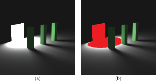
(a) A scene rendered with a rectangular light that touches the plane; (b) out-of-gamut pixels rendered in red.
As an example of how this should be done, Shirley and Morley (2003) discusses the direct illumination from a spherical light using the area form of the rendering equation with a pdf that includes the 1/d2 term. This cancels the term in G(p, p′j). It shows a nice image of two spheres that just touch, where one sphere is emissive. There is no overflow in the reflected radiance, and there shouldn’t be, of course, because the emitted radiance is always finite.
Another way to avoid the overflow problem is to use the hemisphere form of the rendering equation, which doesn’t involve the 1/d2 term (see the Further Reading section and Chapter 26).
18.10 Environment Lights
An environment light is an infinitely large sphere that surrounds a scene and provides illumination from all directions. It’s often used to simulate the diffuse sky illumination for outdoor scenes. The sphere has an emissive material, which can be a constant color or spatially varying. In the latter case, the colors are often based on a physical sky model, or photographs of the sky. In either case, the results can be beautiful images with soft shading.
A number of figures in Chapters 11 and 12 used a large hemisphere with clouds to add interest to the images, but this wasn’t used as an environment light. In those images, rays that didn’t hit any objects brought back a cloud-texture color instead of a constant background color. The Uffizi images in Chapter 11 are similar, except that the only object in the scene is a large textured sphere. In this chapter, I’ll only consider environment lights with a constant color. Chapter 29 will cover textured environment lights.
I haven’t implemented the environment light as an AreaLight because attempting to evaluate the Monte Carlo estimator (18.3) with an infinitely large sphere is problematic. Instead, it’s better to use the hemisphere formulation of the rendering equation, where the shadow rays are distributed in solid angle. We still need to use Monte Carlo integration, as the illumination can come from all directions. The shadow rays are shot with a cosine distribution into the hemisphere that’s oriented around the normal at each hit point because this is suitable for matte materials. Although this only samples half of the sphere directions, for opaque materials, there’s no use sampling the half of the sphere that’s below the tangent plane at the hit point, as these points can’t contribute to the incident radiance (see the Notes and Discussion section).
The Monte Carlo estimator for the integral in Equation (13.21) is
where the pdf p(ωi,j) must now be expressed in terms of a solid-angle measure. In this case, we’ll want to make the pdf proportional to cos θi = n • ωi, to match the cos θi term in the integrand, but it must be normalized. Letting p = c cos θi, where c is the normalization constant, we require
Writing out the integral explicitly gives
from Equation (2.12), and hence
We should implement another tracer to evaluate the estimator (18.4), but to save the work of not only implementing a new tracer class but also of writing new shade functions for all of the materials, I’ve used the AreaLighting tracer. The trick is not to define the Gfunction for the environment light, as this forces the C++ compiler to use the Gfunction defined in the Light base class, which returns 1.0.
Listing 18.14 shows the declaration for the class EnvironmentLight, which doesn’t contain a sphere; the code just works as if there is an infinite sphere.
class EnvironmentLight: public Light {
public:
// constructors etc.
void
set_sampler(Sampler* sampler);
virtual Vector3D
get_direction(ShadeRec& s);
virtual RGBColor
L(ShadeRec& sr);
bool
in_shadow(const Ray& ray, const ShadeRec& sr) const;
virtual float
pdf(const ShadeRec& sr) const;
private:
Sampler* sampler_ptr;
Material* material_ptr;
Vector3D u, v, w;
Vector3D wi;
};
Listing 18.14. The class EnvironmentLight.
Vector3D
EnvironmentLight::get_direction(ShadeRec& sr) {
w = sr.normal;
v = (0.0034, 1, 0.0071) ^ w;
v.normalize();
u = v ^ w;
Point3D sp = sampler_ptr->sample_hemisphere();
wi = sp.x * u + sp.y * v + sp.z * w;
return(wi);
}
Listing 18.15. The function EnvironmentLight::get_direction.
RGBColor
EnvironmentLight::L(ShadeRec& sr) {
return (material_ptr->get_Le(sr));
}
Listing 18.16. The function EnvironmentLight::L.
The classes EnvironmentLight and AmbientOccluder have several features in common. First, their set_sampler functions are the same, where both map the sample points to a hemisphere with a cosine distribution. Second, the mechanism for shooting shadow rays is the same. Both classes have to set up the same u, v, w basis at each hit point, but they do this in different places. Recall from Listing 17.5 that the function AmbientOccluder::L has to set up u, v, and w before it calls the get_direction function. Because the environment light is stored in World::lights, the materials’ area_light_shade functions call EnvironmentLight::get_direction before they call EnvironmentLight::L. We therefore have to set up u, v, and w in get_direction, as shown in Listing 18.15.
The function EnvironmentLight::L is then quite simple, as Listing 18.16 indicates.
Finally, the in_shadow function is the same for both classes, and so I won’t reproduce the EnvironmentLight::in_shadow function here.
Listing 18.17 shows how to construct an environment light. Note that the concave sphere for the direct rendering has a finite but very large radius.
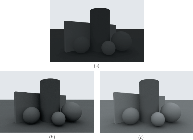
Figure 18.7 shows an example scene, where each part illustrates a different illumination component. The scene contains an environment light with a white emissive material. Figure 18.7(a) is rendered with ambient occlusion only, where each material has a low ambient reflection coefficient so that the images won’t be washed out when we add other illumination components. Figure 18.7(b) is rendered with the environment light but with no ambient illumination. Here, parts of the objects are black where they receive no illumination from the environment light, in the same way that they would be black if they were rendered with ambient occlusion and min_amount = 0. This is no coincidence, as the sampling techniques are the same. Figure 18.7(c) shows the results of using ambient occlusion and the environment light, resulting in a lighter and softer image.
Emissive* emissive_ptr = new Emissive;
emissive_ptr->set_ce(1.0, 1.0, 0.5);
emissive_ptr->set_brightness(1.0);
ConcaveSphere* sphere_ptr = new ConcaveSphere;
sphere_ptr->set_radius(1000000.0);
sphere_ptr->set_material(emissive_ptr);
sphere_ptr->set_shadows(false);
add_object(sphere_ptr);
EnvironmentLight* light_ptr = new EnvironmentLight;
light_ptr->set_material(emissive_ptr);
light_ptr->set_sampler(new MultiJittered(num_samples));
light_ptr->set_shadows(true);
add_light(light_ptr);
Listing 18.17. A build function fragment that constructs an environment light.
A scene rendered with different lighting components: (a) ambient occlusion only; (b) white environment light only; (c) ambient occlusion and environment light. All images were rendered with 100 rays per pixel.
Figure 18.8 shows this scene rendered with a yellow and a blue environment light. As you can see, the color of the light has a dramatic effect on the images.

The scene in Figure 18.7 rendered with ambient occlusion with a yellow environment light (a) and a blue environment light (b).
We can achieve more realistic lighting for outdoor scenes by adding a directional light to simulate direct sunlight. You will be pleased to know that directional and point lights will work without modification with the AreaLighting shader. Figure 18.9 shows the scene in Figure 18.8(a) rendered with an added directional light.

The scene in Figure 18.8(a) rendered with ambient occlusion, a yellow environment light, and an orange directional light, to simulate outdoor lighting conditions just after sunrise or before sunset.
Figure 18.10 shows an environment-light scene without a ground plane, so that the objects are illuminated from all directions. The spheres are from the figure on the first page of Chapter 14 with random colors and rendered from the negative z-axis. They are surrounded by a white environment light and also rendered with ambient occlusion (see Question 17.2). The environment light’s sphere doesn’t cast shadows. This scene provides an opportunity to compare the results of different sampling techniques. Figure 18.10(a) and (b) were rendered with 16 samples per pixel, which is not nearly enough. Multi-jittered sampling was used in Figure 18.10(a) and Hammersley sampling in Figure 18.10(b). The printed images here don’t do justice to the ugliness of these images, which are ugly for different reasons: noise in Figure 18.10(a) and texture-like artifacts in Figure 18.10(b). Figure 18.10(c) and (d) use the same sampling techniques with 256 samples per pixel, which is adequate. In this case, both images are good, there being just a faint hint of artifacts in Figure 18.10(d). You need to look at these images on the book’s website.

Spheres rendered with a white environment light and ambient occlusion: (a) 16 multi-jittered samples for the ambient occlusion and environment light; (c) same as (a) but 256 samples per pixel; (b) 16 Hammersley samples for the ambient occlusion and environment light, (d) same as (a) but 256 samples per pixel.
Notes and Discussion
My spherical light uses a LightSphere object, which is a sphere with a sampler object that distributes sample points over its surface with a uniform density. It does this by calling the function Sampler::map_to_sphere(0). The pdf is p = 1/(4πr2), where r is the radius. This implementation results in noisy images because the cos θ′ term in G(p, p′j varies so much. better implementations are discussed in the references cited in the Further Reading section.
There’s a sampling subtlety with the environment light. Recall from Section 18.10 that although the light represents a sphere that surrounds the scene, the shadow rays are distributed in the hemisphere above each hit point p, where the correct pdf measure is p = cos θi/π. If we were doing volumetric rendering where p is a point in space, we would have to distribute the shadow rays over the whole sphere that surrounds p. In this case, the correct pdf would be p = cos θi/2π because the integral (18.5) would then be over a sphere. Now, we can also use spherical sampling to render opaque surfaces and still get the correct results, but we would need twice as many samples per pixel to reduce the noise to the same levels as hemisphere sampling produces. The reason is as follows. If we used 100 samples per pixel, only 50 of these would be in the hemisphere above p and therefore able to contribute to the incident radiance, but the reflected radiance Lo from each sample would be multiplied by 2π instead of π. The result would therefore be the same as using the hemisphere sampling except for the increase in noise.
In Chapter 21, I’ll discuss how to apply affine transformations to geometric objects, but the technique presented there won’t allow us to transform area lights. For example, if we wanted to translate the rectangular light in Figure 18.4, the rectangle object would be translated, but the illumination would stay the same. The reason is that the sample points would not be translated. This isn’t a serious problem, as the definitions of disks and rectangles allow us to specify arbitrary locations, sizes, and orientations. Nonetheless, one of the exercises in Chapter 21 will ask you to think about how to apply affine transformations to area lights.
The AreaLight::get_direction function in Listing 18.8 calls the geometric object’s get_normal function, which returns the normal given a sample point on its surface. This will work for planar objects, where the normal is part of the object’s definition. It will also work for objects defined by single implicit functions because we can use the gradient operator to compute the normal:
Here, (x, y, z) are the sample-point coordinates. This process will not work for other objects, such as triangle meshes. A solution is to compute and store the normals as the sample points are generated. Geometric information such as the vertex normals can be used for this purpose.
Further Reading
Soft shadows were first rendered with ray tracing by Cook et al. (1984). My area-lighting architecture, where a single area light class contains a pointer to a self-emissive object, is based on the design in Pharr and Humphreys (2004). Some of the implementation details are also based on Dutré et al. (2006). Both of these books contain a comprehensive discussion of ray tracing with area lights.
Shirley and Morley (2003) and Pharr and Humphreys (2004) present techniques for accurately rendering the direct illumination from spherical lights. Shirley’s technique is also discussed in Shirley et al. (2005).
Pharr and Humphreys (2004) discusses a sampling pattern called a (0, 2) sequence, which suffers less distortion than other sampling patterns when it’s mapped onto long thin rectangles. As such, it may be better than multi-jittered sampling for shading with thin rectangular lights, but, like Hammersley patterns, it’s not random. The original literature on this pattern is the book by Niederreiter (1992) and the paper by Kollig and Keller (2002).
Although we can use as many area lights as we like in a given scene, the amount of sampling will be proportional to the number of lights multiplied by the number of samples per pixel. Shirley et al. (1996) developed techniques for efficiently sampling large numbers of area lights. See also Shirley and Morley (2003).
There’s a lot more to rendering with area lights than I’ve presented here, where all the images in the preceding sections were rendered by sampling the light sources and the BRDFs were Lambertian. Pharr and Humphreys (2004) discusses rendering with area lights by sampling the BRDF, which can often work better for specular BRDFs. Of course, scenes can have any combination of BRDFs that range from Lambertian to perfect specular, and area lights that range from small to the whole hemisphere. To handle this situation, a technique called multiple importance sampling was developed by Veach and Guibas (1995). See also Veach’s PhD thesis (1997). Pharr and Humphreys (2004) has a clear discussion of this for the special case of two BRDFs.
Questions
- 18.1. Why do the edges of the area lights in Figure 18.4, Figure 18.5 and Figure 18.6 appear as if they haven’t been antialiased?
- 18.2. Why doesn’t the function EnvironmentLight::L in Listing 18.16 have to check that the light is being emitted on the inside surface of the sphere?
- 18.3. How do directional and area lights work without modification with the area_light_shade functions?
- 18.4. Figure 18.11 shows the scene from Figure 18.7(c) rendered with Phong materials on all objects except the plane. The Phong materials have a red specular color, and the specular exponent varies from 10 to 200. Notice how the specular highlights decrease in brightness as the exponent increases and almost disappear when e = 200. Can you explain this? Is there a solution?

Exercises
- 18.1. Here’s a simple way to produce soft shadows with a point light. Just jitter the light’s location in 3D as in Listing 18.18. I’ve called this FakeSphericalLight, although the jittered locations are actually in an axis-aligned cube of edge length 2r. That doesn’t matter much because of the soft shadows’ insensitivity to area-light shapes, as Figures 18.5 and 18.6 demonstrate. The value of r will depend on the light’s location and how soft you want the shadows to be.
As far as the direct illumination is concerned, this light is a rudimentary simulation of a cubic volume light using multiple point lights, but it will be directly rendered as a self-emissive sphere.
Figure 18.12(a) shows the scene in Figure 18.5(b) rendered with r = 3.0 and distance attenuation. The scene contains a sphere with an emissive material centered at the light’s location and with radius r, the same as the scene in Figure 18.5(b). Comparing the two figures, which were both rendered with 100 rays per pixel, shows that the shadows are almost identical, but Figure 18.12(a) contains a lot less noise than 18.5(b). There are two reasons for this. First, the fake spherical light’s locations are in a 3D volume, while the spherical light’s sample points in 18.5(b) are on the surface of a sphere. Second, my implementation of the spherical light is crude and subject to a lot of noise. As a result, Figure 18.12(b) is actually the better looking of the two images. Figure 18.12(b) shows the scene rendered without distance attenuation. There is a large difference in the brightness values between these two images, where ls = 250.0 in Figure 18.12(a) and ls = 3.0 in Figure 18.12(b).

Illumination from a fake spherical light with distance attenuation (a) and with no distance attenuation (b).
Implement a fake spherical light.
Vector3DFakeSphericalLight::get_direction(ShadeRec& sr) {float r = 3.0;Point3D new_location;new_location.x = location.x + r * (2.0 * rand_float() - 1.0);new_location.y = location.y + r * (2.0 * rand_float() - 1.0);new_location.z = location.z + r * (2.0 * rand_float() - 1.0);return ((new_location - sr.hit_point).hat());}Listing 18.18. The function FakeSphericalLight::get_direction.
- 18.2. We can be a bit more “honest” with the fake spherical light by restricting the locations to lie in a sphere instead of a cube. Implement a rejection-sampling technique to enforce this, but make sure that every time FakeSphericalLight::get_direction is called, it does return a direction. Compare the results with Figure 18.12.
- 18.3. Implement a jittered directional light. The figure on the first page of this chapter was rendered with this type of light.
- 18.4. Implement a rectangular area light as described in this chapter and use the figures in Section 18.7 to test your implementation.
- 18.5. Implement a disk light and use Figure 18.5(a) to test your implementation. In contrast to the rectangular light, you will need to set up a (u, v, w) basis to compute the sample-point coordinates.
- 18.6. Experiment with other sampling techniques and numbers of rays per pixel for the figures in Section 18.9.
- 18.7. The figures in Section 18.9 were rendered with shadows set to false for the rectangle, disk, and sphere. Render the figures with shadows set to true for these objects and compare the results.
- 18.8. Render some scenes with shadows turned off for the area lights.
- 18.9. Render the scene in Figure 18.4(a) with a rectangular light of aspect ratio 2 : 1 and two square lights, side-by-side and with the same total area, and compare the results.
- 18.10. Implement an option on the AreaLight class that will allow you to specify the total power of the light as a quantity that’s independent of the surface area. This is more convenient for scene design than the current implementation, where the power is proportional to the area.
- 18.11. Implement an environment light as described in Section 18.10 and use the figures there to test your implementation.
- 18.12. Implement the function area_light_shade for the Phong material and reproduce Figure 18.11. Experiment with different values of the Phong exponent e.
- 18.13. Reproduce the images in Figure 18.10, and experiment with different scene parameters such as the number of samples, the sampling technique, environment-light color, ambient-light conditions, and the material properties of the spheres. You can mix and match different sampling techniques for antialiasing, ambient occlusion, and the environment light.
- 18.14. Produce some nice images of your own with area and environment lights.
1. Direct lighting is another common name for direct illumination.
2. In this context, isotropic means that the emitted radiance is the same in all directions at every point on the light surface.
3. SV_Emissive is a spatially varying version of Emissive that will allow us to render scenes with textured area lights in Chapter 29.
4. The light surface has also overflowed because the scene was rendered with ls = 40, but that’s all right: ls can be as large as we need to provide adequate illumination to the objects in the scene.