
Chapter 3
Bare-Bones Ray Tracing

Objectives
By the end of this chapter, you should:
- understand how ray casting works;
- know how rays are defined;
- know how to intersect a ray with a plane and a sphere;
- understand the structure of a simple ray tracer;
- have implemented a ray tracer that can render orthographic views of an arbitrary number of planes and spheres.
The purpose of this chapter is to explain how a number of ray-tracing processes work in a simplified context. I’ll discuss here how ray tracing generates images, how rays are defined, how ray-object intersections work, the classes required for a simple ray tracer, and how to ray trace an arbitrary number of spheres and planes. To make things as simple as possible, I’ve left out a lot of important processes such as antialiasing, perspective viewing with a pinhole camera, and shading. By doing this, the resulting ray tracer is as simple as possible, although, as you’ll see, it still has a degree of complexity. This is also a long chapter because it covers a lot of material.
This chapter differs from the following chapters in that the skeleton ray tracer on the book’s website does everything in the chapter. Hopefully, this will have you quickly ray tracing multiple planes and spheres.
3.1 How Ray Tracing Works
A simple ray tracer works by performing the following operations:
define some objects
specify a material for each object
define some light sources
define a window whose surface is covered with pixels
for each pixel
shoot a ray towards the objects from the center
of the pixel
compute the nearest hit point of the ray with the
objects (if any)
if the ray hits an object
use the object’s material and the lights to
compute the pixel color
else
set the pixel color to black
This is known as ray casting. Figure 3.1 illustrates some of the above processes for a sphere, a triangle, and a box, illuminated by a single light. The gray rectangles on the left are the pixels, and the white arrows are the rays, which start at the center of each pixel. Although there is one ray for each pixel, Figure 3.1 only shows a few rays. The red dots show where the rays hit the objects. The rays used in ray tracing differ from real light rays (or photons) in two ways. First, they travel in the opposite direction of real rays. This is best appreciated when we use a pinhole camera (Chapter 9), because there the rays start at the pinhole, which is infinitely small. If the rays started at the lights, none of them would pass through the pinhole, and we wouldn’t have any images. Starting the rays from the camera (or pixels, in this chapter) is the only practical way to render images with ray tracing. The second difference is that we let the rays pass through the objects, even if they are opaque. We have to do this because the ray tracer needs to intersect each ray with each object to find the hit point that’s closest to the start of the ray.

Rays shot from pixels into a scene that consists of three objects and a single light source.
In Figure 3.1, one ray doesn’t hit any objects, two rays hit one object, and one ray hits two objects. The hit points are always on the surfaces of the objects, which we treat as empty shells. As a result, rays hit the sphere and the box in two places and the triangle in one place.
The pixels are on a plane called the view plane, which is perpendicular to the rays. I’ll sometimes refer to these as view-plane pixels. The rays are parallel to each other and produce an orthographic projection of the objects. When a ray hits an object, the color of its pixel is computed from the way the object’s material reflects light, a process that’s known as shading. Although the pixels on the view plane are just mathematical abstractions, like everything else in the ray tracer, each one is associated with a real pixel in a window on a computer screen. This is how you view the ray-traced image.
The process of working out where a ray hits an object is known as the ray-object intersection calculation. This is a fundamental process in ray tracing and usually takes most of the time. The intersection calculation is different for each type of object; some objects are easy to intersect, while others are difficult. All intersection calculations require some mathematics.
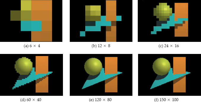
In Figure 3.1, there are 24 pixels arranged in four rows of six pixels, and in this case we say the image has a pixel resolution of 6 × 4. What would these objects look like if we ray traced them at this resolution? The result is in Figure 3.2(a), which gives no indication of what we are looking at. So, how can we get a meaningful image of these objects? The answer is simple: just increase the number of pixels. The other parts of Figure 3.2 show the objects ray traced at increasing pixel resolutions. With 24 × 16 pixels, we have some idea of what the objects are, and with 150 × 100 pixels, the image is quite good.
The above example was just to illustrate how ray tracing works with multiple objects, a light source, and shading. We’ll start with something much simpler in Section 3.6: a single sphere with no lights, no material, and no shading, but first you need to learn how a basic ray tracer is organized and works.
3.2 The World
Ray tracers render scenes that contain the geometric objects, lights, a camera, a view plane, a tracer, and a background color. In the ray tracer described in this book, these objects are all stored in a world object. For now, the world will only store the objects and view plane. The locations and orientations of all scene elements are specified in world coordinates, which is a 3D Cartesian coordinate system, as described in Chapter 2. I’ll denote world coordinates by (xw, yw, zw), or just (x, y, z) when the context is clear.
World coordinates are known as absolute coordinates because their origin and orientation are not defined, but that’s not a problem. The only task of the ray tracer is to compute the color of each pixel, and the pixels are also defined in world coordinates. I’ll discuss the World class in Section 3.6.
3.3 Rays
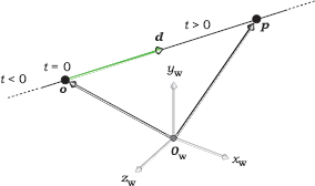
A ray is an infinite straight line that’s defined by a point o, called the origin, and a unit vector d, called the direction. A ray is parametrized with the ray parameter t, where t = 0 at the ray origin, so that an arbitrary point p on a ray can be expressed as
Figure 3.3 is a schematic diagram of a ray. The direction d defines an intrinsic direction for the ray along the line, where the value of the parameter t increases in the direction d. Since d is a unit vector, t measures distance along the ray from the origin. Although we regard a ray as starting at its origin, we allow t to lie in the infinite interval t ∊ (−∞, +∞) so that Equation (3.1) generates an infinite straight line. As we’ll see later, it’s essential to consider values of t ∊ (−∞, +∞) in ray-object intersections. The origin and direction are always expressed in world coordinates before the ray is intersected with the objects.
Ray tracing uses the following types of rays:
- primary rays;
- secondary rays;
- shadow rays;
- light rays.
Primary rays start at the centers of the pixels for parallel viewing, and at the camera location for perspective viewing. Secondary rays are reflected and transmitted rays that start on object surfaces. Shadow rays are used for shading and start at object surfaces. Light rays start at the lights and are used to simulate certain aspects of global illumination, such as caustics. I’ll only discuss primary rays in this chapter.
You should have a Ray class that stores the origin and direction, as in Listing 3.1. Because of their frequent use, all data members are public. In my shading architecture, there’s no need to store the ray parameter in the ray. The code in Listing 3.1 will go in the header file Ray.h. Note the pre-compiler directives #ifndef__RAY__, etc., to prevent multiple inclusion. These should go in every header file, but to save space, I won’t quote them with other class declarations. You should also #inlcude header files for any classes that the current class requires: Point.h and Vector3D in this case. Again, to save space, I’ll leave these out except for the World class in Section 3.6.1.
#ifndef__RAY__
#define__RAY__
#include “Point3D.h”
#include “Vector3D.h”
class Ray {
public:
Point3D o; // origin
Vector3D d; // direction
Ray(void); // default constructor
Ray(const Point3D& origin, const Vector3D& dir); // constructor
Ray(const Ray& ray); // copy constructor
Ray& // assignment operator
operator= (const Ray& rhs);
~Ray(void); // destructor
};
#endif
Listing 3.1. The Ray.h file.
3.4 Ray-Object Intersections
3.4.1 General Points
The basic operation we perform with a ray is to intersect it with all geometric objects in the scene. This finds the nearest hit point, if any, along the ray from o in the direction d. We look for the hit point with the smallest value of t in the interval t∊[ε, +∞) where ε is a small positive number, say ε = 10−6. Why don’t we use ε = 0? We could get away with this here, but it would create problems when we use shadows (Chapter 16), reflections (Chapter 24, Chapter 25 and Chapter 26), and transparency (Chapters 27 and 28). I’ll discuss what the problem is in Chapter 16. By using ε > 0 in this chapter, we won’t have to change the plane and sphere hit functions in later chapters.
Because a ray origin can be anywhere in the scene, including inside objects and on their surfaces, ray-object hit points can occur for positive, negative, and zero values of t. This is why we need to treat rays as infinite straight lines instead of semi-infinite lines that start at o. Figure 3.4(a) shows a number of spheres that are behind, straddling, and in front of the view plane, with three rays.
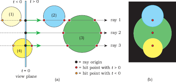
The spheres in Figure 3.4(a) will be rendered (or not) in the following ways:
- Sphere (1) is behind the origin of all rays that intersect it (t < 0) and will not appear in the image.
- Sphere (2) will be rendered with ray 1 and with all rays that hit it.
- Sphere (3) will only be rendered with rays like ray 2 that don’t hit any other spheres.
- Sphere (4) will only be rendered with rays like ray 3 that start inside it.
Figure 3.4(b) shows how the spheres would look if we ray traced them with no shading and if their centers were all in the vertical plane that contains the three rays. The nearest hit points of these rays are indicated in the figure.
3.4.2 Rays and Implicit Surfaces
As I discussed in the previous chapter, the objects we ray trace are defined by implicit surfaces. A ray can hit an implicit surface any number of times, depending on how complex the surface is (see Figure 3.5). If the surface is closed, rays that start outside the surface will have an even number of hit points for t > ε (rays 1 and 2). In principal, a ray that starts outside can have an odd number of hit points, including a single hit point, if it hits the surface tangentially (rays 3 and 5). In practice, this rarely happens (see Question 3.1). When the ray starts inside the surface, it will have an odd number of hit points for t > ε (ray 4).

To intersect a ray with an implicit surface, we can re-write Equation (2.5), f (x, y, z) = 0, as
because the x, y, and z variables in f (x, y, z) define a 3D point p = (x, y, z).
To find the hit points, we have to find the values of the ray parameter t that correspond to them. How do we do this? Here’s the key point: Hit points satisfy both the ray equation (3.1) and the implicit surface equation (3.2). We can therefore substitute (3.1) into (3.2) to get
as the equation to solve for t. Since Equation (3.3) is symbolic, we can’t do anything with it unless we specify f (x, y, z). For a given ray and a given implicit surface, the only unknown in Equation (3.3) is t. After we have found the values of t, we substitute the smallest t > ε value into Equation (3.1) to find the coordinates of the nearest hit point. If all this seems confusing, don’t worry, because I’m going to illustrate it for planes and spheres. For these objects, we can solve Equation (3.3) exactly.
3.4.3 Geometric Objects
All geometric objects belong to an inheritance structure with class GeometricObject as the base class. This is by far the largest inheritance structure in the ray tracer, with approximately 40 objects, but in this chapter we’ll use a simplified structure consisting of GeometricObject, Plane, and Sphere, as shown on the left of Figure 1.1.
class GeometricObject {
public:
...
virtual bool
hit(const Ray& ray, double& tmin, ShadeRec& sr)
const = 0;
protected:
RGBColor color; // only used in this chapter
};
Listing 3.2. Partial declaration of the GeometricObject class.
Listing 3.2 shows part of the GeometricObject class declaration that stores an RBGColor for use in Section 3.6. I’ll replace this with a material pointer when I discuss shading in Chapter 14. This listing also doesn’t show other functions that this class must have in order to operate as the base class of the geometric objects hierarchy, but it does show the declaration of the pure virtual function hit.
class ShadeRec {
public:
bool hit_an_object; // did the ray hit an object?
Point3D local_hit_point; // world coordinates of hit point
Normal normal; // normal at hit point
RGBColor color; // used in Chapter 3 only
World& w; // world reference for shading
ShadeRec(World& wr); // constructor
ShadeRec(const ShadeRec& sr); // copy constructor
~ShadeRec(void); // destructor
ShadeRec& // assignment operator
operator= (const ShadeRec& rhs);
};
ShadeRec::ShadeRec(World& wr) // constructor
: hit_an_object(false),
local_hit_point(),
normal(),
color(black),
w(wr)
{}
Listing 3.3. Declaration of the ShadeRec class.
The ShadeRec object in the parameter list of the hit function is a utility class that stores all of the information that the ray tracer needs to shade a ray-object hit point. Briefly, shading is the process of computing the color that’s reflected back along the ray, a process that most of this book is about. The ShadeRec object plays a critical role in the ray tracer’s shading procedures, as this chapter starts to illustrate in a simplified context. Listing 3.3 shows a declaration of the ShadeRec class with the data members that we need here. Note that one data member is a world reference. Although this is only used for shading, I’ve included it here, as it prevents the ShadeRec class from having a default constructor; the reference must always be initialized when a ShadeRec object is constructed (Listings 3.14 and 3.16) or copy constructed (Listing 3.17). Listing 3.3 includes the ShadeRec constructor code (see also the Notes and Discussion section). I haven’t included an assignment operator, as the ray tracer is written in such a way that it’s not required. For example, no class has a ShadeRec object as a data member.
3.4.4 Planes
Planes are the best geometric objects to discuss first because they are the easiest to intersect. To do this, we first substitute Equation (3.1) into the plane equation (2.6),
to get
This is a linear equation in the ray parameter t whose solution is
A linear equation has the form
where a and b are constants, and t is an unknown variable. The solution is
See Exercise 3.10.
Because linear equations have a single solution, Equation (3.4) tells us that a ray can only hit a plane once. We could now substitute the expression (3.4) for t into Equation (3.1) to get a symbolic expression for the hit-point coordinates, but we don’t do this for two reasons. First, we don’t need the hit-point coordinates until we shade the point, and we only do that for the closest point to the ray origin. We won’t know what that point will be until we’ve intersected the ray with all of the objects. Second, it’s more efficient to calculate the numerical value of t from Equation (3.4) and substitute that into (3.1) to get numerical values for the coordinates. This applies to all geometric objects. The ray tracer must have numerical values for shading.
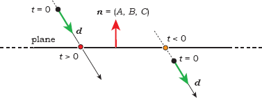
Figure 3.6 shows an edge-on view of a plane with two rays. The ray on the left hits the plane with t > ε, but the ray on the right hits it with t < 0. We must check that the value of t in Equation (3.4) satisfies t > ε before recording that an intersection has occurred. In this context, it doesn’t matter whether the normal to the plane points up or down in Figure 3.6, as this will only affect the shading.
class Plane: public GeometricObject {
public:
Plane(void);
Plane(const Point3D p, const Normal& n);
...
virtual bool
hit(const Ray& ray, double& t, ShadeRec& s) const;
private:
Point3D point; // point through which
// plane passes
Normal normal; // normal to the plane
static const double kEpsilon; // see Chapter 16
};
Listing 3.4. The Plane::hit function.
bool
Plane::hit(const Ray& ray, double& tmin, ShadeRec& sr) const {
double t = (point - ray.o) * normal / (ray.d * normal);
if (t > kEpsilon) {
tmin = t;
sr.normal = normal;
sr.local_hit_point = ray.o + t * ray.d;
return (true);
}
else
return (false);
}
Listing 3.5. The Plane::hit function.
What happens if the ray is parallel to the plane? In this case, d • n = 0, and the value of the expression (3.4) is infinity. Is this a problem? Not if you are programming in C++, because floating-point calculations in this language satisfy the IEEE floating-point standard, where division by zero returns the legal number INF(infinity). As a result, there’s no need to check for d • n = 0 as a special case; your ray tracer will not crash if it divides by zero.
The class Plane stores the point and the normal. Its declaration appears in Listing 3.4 with two constructors; each class should have a default constructor, and other constructors as required.
Listing 3.5 shows the ray-plane hit function. Ray-object hit functions don’t come any simpler than this.
All object hit functions compute and return information in three ways: their return type is a bool that indicates if the ray hits the object; they return the ray parameter for the nearest hit point (if any) through the parameter tmin; they return information required for shading with the ShadeRec parameter. We won’t need the normal until shading in Chapter 14, and we won’t need the hit point local_hit_point until texturing in Chapter 29. By including them now, we won’t have to change this hit function later on.
3.4.5 Spheres
Equation (2.8) for a sphere can be written in vector form as
(see Exercise 3.11). To intersect a ray with a sphere, we substitute Equation (3.1) into (3.5) to get
Expanding Equation (3.6) gives
Equation (3.7) is a quadratic equation for t, which we can write as
where1
The solution to Equation (3.8) is given by the standard expression
Quadratic equations can have zero, one, or two real roots, depending on the value of the discriminant
This is reflected in the fact that a ray can hit a sphere zero, one, or two times (see Figure 3.7). Here, ray 1 does not hit the sphere (d < 0), ray 2 has one hit point with t ∊ [ε, +∞) (d = 0) because it hits the sphere tangentially, and ray 3 has two hit points with t ∊ [ε, +∞) (d > 0).

bool
Sphere::hit(const Ray& ray, double& tmin, ShadeRec& sr) const {
double t;
Vector3D temp = ray.o - center;
double a = ray.d * ray.d;
double b = 2.0 * temp * ray.d;
double c = temp * temp - radius * radius;
double disc = b * b - 4.0 * a * c;
if (disc < 0.0)
return(false);
else {
double e = sqrt(disc);
double denom = 2.0 * a;
t = (-b - e) / denom; // smaller root
if (t > kEpsilon) {
tmin = t;
sr.normal = (temp + t * ray.d) / radius;
sr.local_hit_point = ray.o + t * ray.d;
return (true);
}
t = (-b + e) / denom; // larger root
if (t > kEpsilon) {
tmin = t;
sr.normal = (temp + t * ray.d) / radius;
sr.local_hit_point = ray.o + t * ray.d;
return (true);
}
}
return (false);
}
Listing 3.6. Ray-sphere hit function.
Although we only need the situations shown in Figure 3.7 in this chapter, the ray-sphere hit function must also give correct answers for the situations shown in Figure 3.8. Since ray 1 in this figure only hits the sphere with t < 0, this ray has zero intersections with the sphere. Because ray 2 starts on the surface of the sphere and d points out of the sphere, one hit point has t = 0 (at least in theory), and the other has t < 0. Therefore, this ray also has zero intersections. Ray 3 starts inside the sphere and has one hit point with t > 0 and one with t < 0, and therefore has one intersection. Finally, ray 4 also starts on the surface, but d points into the sphere. This ray, therefore, has one intersection. Rays 2 and 4 could be reflected, transmitted, or shadow rays, and as we’ll see in later chapters, it’s critical that these rays do not record an intersection at their origins.

The ray-sphere hit function in Listing 3.6 correctly handles all of the above situations, but note that we don’t test for tangential intersection when d = 0 (see Question 3.2).
3.5 Representing Colors
As ray tracing is all about computing the color of each pixel, we need a way to represent and store colors. One of the most remarkable aspects of our perception of color is that it’s three dimensional. We can therefore specify colors in 3D color spaces. There are a number of these in common use, but the one that’s most aligned to graphics monitors is called RGB, which is short for red, green, and blue.
What does the RGB color space look like? First, there are three axes (r, g, b) defined by the red, green, and blue colors. These form a right-handed coordinate system, except that there are no negative values, and (r, g, b) ∊ [0, 1]3. The RGB color space, the set of all legal values of r, g, and b, is therefore a unit cube with one vertex at the (r, g, b) origin (see Figure 3.9). It’s therefore called the RGB color cube.

Pure red, green, and blue are known as the additive primary colors and are represented by r = (1, 0, 0), g = (0,1,0), and b = (0, 0, 1). They have the following properties (see Figure 3.10):

Figure 3.11 shows some views of the RGB color cube. Yellow, cyan, and magenta are known as secondary colors and are at the three cube vertices that lie in the (r, g, b) coordinate planes, as indicated in Figure 3.11(a). These are also the CMY subtractive primary colors, used for printing (see Figure 28.8).

(a) Isometric view of the RGB color cube; (b) surface of the cube that’s in the (r, g) plane; (c) the cube sliced in half by a plane through the blue axis.
Figure 3.11(b) is the surface of the cube that lies in the (r, g) plane, and it shows all combinations of red and green with no blue. For example, the orange color (1, 0.5, 0) is half way along the right boundary of the square. Colors along the red axis are (r, 0, 0), with r ∊ [0, 1], and range from black to pure red. Similarly, all combinations of red and blue are on the surface of the cube in the (r, b) plane, and all combinations of green and blue are on the surface in the (g, b) plane.
Figure 3.11(c) shows the cube sliced in two by a plane that contains the blue axis and that passes through (1, 1, 1). Grays lie along the diagonal dashed line from black to white, but it’s not possible to see them in this figure, as the line from (0, 0, 0) to (1, 1, 1) is, of course, infinitely thin. Grays have all components the same; that is, gray = (a, a, a), where a ∊ (0, 1). For example, a medium gray is (0.5, 0.5, 0.5).
I’ll store RGB colors in the RGBColor class, which represents the components with an ordered triple of floating-point numbers r, g, b. Let
be three colors, and let a and p be floating-point numbers. We will need the following operations:
Operation |
Definition |
Return Type |
|---|---|---|
c1 + c2 |
(r1 +r2, g1 + g2, b1 +b2) |
RGB color |
ac |
(ar, ag, ab) |
RGB color |
ca |
(ar, ag, ab) |
RGB color |
c / a |
(r / a, g / a, b / a) |
RGB color |
c1 = c2 |
(r1 = r2, g1 = g2, b1 = b2) |
RGB color reference |
c1 * c2 |
(r1 r2, g1 g2, b1 b2) |
RGB color |
cp |
(rp, gp, bp) |
RGB color |
c1 += c2 |
(r1 += r2, g1 += g2, b1 += b2) |
RGB color reference |
The operator c1* c2 is component-wise multiplication of two colors; it’s used for color mixing. For convenience, I’ve defined black, white, and red as constants in the Constants.h file.
The ray tracer will compute an RGB color for each pixel, but before you can display these on your computer screen, they must be converted to the representation that your computer uses for display purposes. This process is platform-dependent and can involve arcane code. You don’t have to worry about this, as the skeleton program does the conversion for Windows machines. I will discuss some display issues in Section 3.8, but we also have to be able to handle color values that are outside the color cube. As these can occur during shading operations, I’ll discuss that in Section 14.9. The skeleton program also allows you to save the images in various file formats, such as JPEG and TIFF.
3.6 A Bare-Bones Ray Tracer
It’s now time to do some ray tracing. With all the preceding mathematics and theory, you may be feeling a little intimidated. If that’s the case, don’t worry, because we are going to start with the simplest possible bare-bones ray tracer. This ray traces an orthographic view of a single sphere centered on the origin of the world coordinates. If a ray hits the sphere we color the pixel red, otherwise we color it black. As the skeleton ray tracer does this, you don’t have to program it unless you want to; you only have to get it running.
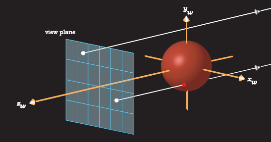
Figure 3.12 shows how the view plane, the world coordinate axes, and the sphere are arranged. This also shows a ray that hits the sphere and a ray that misses it.
3.6.1 Required Classes
Just to ray trace this simple scene, we need the following 12 classes:
Geometric Objects |
Tracers |
Utility |
World |
|---|---|---|---|
GeometricObject Sphere |
Tracer SingleSphere |
Normal Point3D Ray RGBColor ShadeRec Vector3D |
ViewPlane World |
These are in the skeleton program. The World, ViewPlane, ShadeRec, and GeometricObject classes are in simplified form at this stage.
Listing 3.7 shows the declaration of a simple World class that’s in the file World.h. This version contains all of the data members and member functions that we need at present. The sphere is a temporary measure for this section only. All data members of World are public. The background color is the color returned by rays that don’t hit any geometric objects. Its default color is black, which is also the default color of an RGBColor object.
Listing 3.8 shows part of the World class definition in the file World.cpp. An important thing to note here are the #include statements. The World.cpp file should contain the header files for all classes used in the ray tracer, except those #included in World.h; by doing this, there shouldn’t be any unknown classes during compilation. I also #include the build functions here, as a simple way to manage them. The code for each build function is in a separate file and #included in World.cpp after all the classes have been #included. All build functions are commented out except for the one currently running. Depending on which development environment you use, you may also need to #include various system header files.
#include “ViewPlane.h”
#include “RGBColor.h”
#include “Sphere.h”
#include “Tracer.h”
class World {
public:
ViewPlane vp;
RGBColor background_color;
Sphere sphere;
Tracer* tracer_ptr;
World(void);
void
build(void);
void
render_scene(void) const;
void
open_window(const int hres, const int vres) const;
void
display_pixel(const int row,
const int column,
const RGBColor& pixel_color) const;
};
Listing 3.7. A simple World class declaration.
#include “Constants.h” // contains kEpsilon and kHugeValue
// utilities
#include “Vector3D.h”
#include “Point3D.h”
#include “Normal.h”
#include “Ray.h”
#include “World.h”
// build functions
#include “BuildRedSphere.cpp” // builds the red sphere
// World member function definitions ...
Listing 3.8. Part of the World.cpp file that contains the #include statements.
3.6.2 The Main Function
In a pure C++ ray tracer with no user interface, the build function would be called from the main function, as shown in Listing 3.9. Depending on your development environment, there may not be a main function as such, but the code that’s in Listing 3.9 will have to appear somewhere.
int
main(void) {
World w; // construct a default world object
w.build();
w.render_scene();
return(0);
}
Listing 3.9. The main function.
class ViewPlane {
public:
int hres; // horizontal image resolution
int vres; // vertical image resolution
float s; // pixel size
float gamma; // monitor gamma factor
float inv_gamma; // one over gamma
...
};
Listing 3.10. The ViewPlane class.
3.6.3 The View Plane
The ViewPlane class stores the number of pixels in the horizontal and vertical directions, along with their size (see Listing 3.10). I’ll discuss the gamma data member in Section 3.8. In later chapters, we’ll store additional data members in this class.
The view plane contains the pixels that form a window through which the scene is rendered. In this chapter, the view plane is perpendicular to the zw-axis, the pixels are arranged in horizontal rows, and the window is centered on the zw-axis. Figure 3.13 is a schematic diagram of the pixels for an 8 × 6 window. Here, the zw-axis would stick out of the paper through the middle of the window (the center dot). The window can also cut the zw-axis at any suitable location. Notice how the rows and columns of pixels are parallel to the xw- and yw-axes, which can be behind or in front of the view plane.
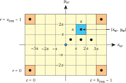
Here, a single ray starts at the center of each pixel, as indicated by the black circles on some pixels. We specify the zw-coordinate for the ray origins, which are all the same, but we have to calculate the xw- and yw-coordinates. As each pixel is a square of size s × s, these coordinates are proportional to s. We number the pixel rows from 0 to vres − 1, from bottom to top, and the columns from 0 to hres − 1, from left to right, as indicated in Figure 3.13. The values of hres and vres are always even, so that the zw-axis goes through the corners of the four center pixels.
Given the above conditions, the expressions for the (xw, yw)-coordinates of the ray origins are
These are simple to derive (see Exercise 3.13).
The ray directions are all d = (0, 0, −1) because the rays travel in the negative zw-direction.
3.6.4 Pixels and Pictures
In a general viewing situation, the part of the scene that’s visible through the window is known as the field of view. In the arrangement here, the field of view depends only on the number of pixels in the horizontal and vertical directions, and their size, because these factors determine the physical dimensions of the window: width shres, and height svres. They also determine where the rays are and, hence, where the scene is sampled. Let me illustrate this with the objects in Figure 3.2. Figure 3.14 shows these objects with three different windows superimposed. Here, the pixels are the same size in each window, but their numbers are different. If we change hres or vres, or both, the shape and size of the window changes accordingly. In each case, the only part of the scene that will be rendered is the part that’s projected through the window. If we rendered the scene in Figure 3.14(a), the result would be the same as Figure 3.2 (a).
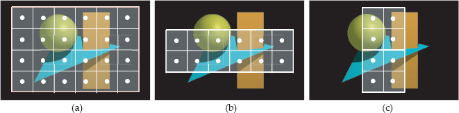
Windows with different pixel resolutions superimposed on a scene: (a) 6 × 4; (b) 6 × 2; (c) 2 × 4. The white dots are the ray origins and indicate where the scene is sampled.
In contrast, Figure 3.15 shows the 6 × 4 pixel window in Figure 3.14(a) with pixels of different size. In Figure 3.15(a), the pixel size s has been reduced by a factor of 2, and in Figure 3.15(b), it’s been reduced by another factor of 2. This results in a most useful process, but see if you can think what it is before reading further.

The windows that result when we reduce the size of the pixels: (a) s is one-half the size it is in Figure 3.14(a); (b) s is one-quarter the size.
Because the part of the scene projected through the window decreases as the pixel size gets smaller, decreasing s zooms into the view. For fixed values of hres and vres, this is the only way we can zoom with an orthographic projection. The process is analogous to zooming with a real camera.
Let’s look now at a different process. Suppose the window you are using gives a good view of a scene, but you aren’t using enough pixels. Figure 3.14(a) might be an example. You can increase the number of pixels, and keep the window the same size, by making the pixels smaller by a corresponding amount. An example is to increase the horizontal and vertical resolutions by two and to make the pixel size half as big. Figure 3.16 shows the window from Figure 3.14(a) with hres = 24 and vres = 16. I’ve used this process to render the images in Figure 3.2.

The window in Figure 3.14(a) with a pixel resolution of 12 × 8. This results in Figure 3.2(b).
Of course, the size of the view-plane pixels doesn’t affect the size of the image on your computer screen. When you display the image, each view-plane pixel is still associated with a real pixel on your screen, regardless of the value of s. The only thing that affects the physical size of the image is the pixel resolution hres × vres and the physical size of the screen pixels.
To illustrate the zooming process, Figure 3.17 shows the views though the two windows in Figure 3.15, rendered at a pixel resolution of 660 × 440, but with view-plane pixels of different size. These images will be the same physical size on your computer screen.

Zoomed views of the objects in Figure 3.2. The pixel size in (a) is 0.26, and in (b) it’s 0.13.
3.6.5 The Build Function
Listing 3.11 shows the build function that I’ll use first, which sets parameters for the view plane and the sphere. Notice that although the data members of the view plane are public, I’ve used set functions to specify the image resolution and pixel size. This allows a uniform notation for constructing objects; some “set” functions require more than a simple assignment statement to perform their tasks. A simple example is the set_gamma function, which also sets inv_gamma.
void
World::build(void) {
vp.set_hres(200);
vp.set_vres(200);
vp.set_pixel_size(1.0);
vp.set_gamma(1.0);
background_color = black;
tracer_ptr = new SingleSphere(this);
sphere.set_center(0.0);
sphere.set_radius(85.0);
}
Listing 3.11. The World::build function.
3.6.6 Rendering the Scene
The function World::render_scene is responsible for rendering the scene.2 Its code appears in Listing 3.12. After storing the image resolution in local variables, it opens a window on the computer screen by calling the function open_window. The main work in render_scene is carried out in the for loops, where the color of each pixel is computed. In this example, the view plane is located at zw = 100, which is hard-wired in. This is, of course, bad programming, but it’s a temporary measure for this chapter. The scene is rendered row-by-row, starting at the bottom-left of the window. Although the render_scene function in the skeleton ray tracer looks the same as Listing 3.12, it writes the pixel colors to an off-screen array and buffers the output.
void
World::render_scene(void) const {
RGBColor pixel_color;
Ray ray;
double zw = 100.0; // hard wired in
double x, y;
open_window(vp.hres, vp.vres);
ray.d = Vector3D(0, 0, -1);
for (int r = 0; r < vp.vres; r++) // up
for (int c = 0; c <= vp.hres; c++) { // across
x = vp.s * (c - 0.5 * (vp.hres - 1.0));
y = vp.s * (r - 0.5 * (vp.vres - 1.0));
ray.o = Point3D(x, y, zw);
pixel_color = tracer_ptr-<trace_ray(ray);
display_pixel(r, c, pixel_color);
}
}
Listing 3.12. The World::render_scene function.
After the ray’s origin and direction have been computed, the function trace_ray is called. This is a key function in the ray tracer because it controls how rays are traced through the scene and returns the color for each pixel. But instead of being called directly, this function is called through a Tracer object called tracer_ptr. See Listing 3.7 and the following section. The last thing the loops do is display the pixel in the window using the display_pixel function. This converts the RGBColor to the display format used by the computer.
OK, that’s enough theory, code, and discussion. Let’s ray trace the sphere and look at the result in Figure 3.18. This is an impressive image when you consider how many things have to work together to produce it.

3.7 Tracers
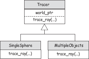
Tracers allow us to implement different types of ray tracing with different versions of the function trace_ray, without altering the existing code. They thus provide a critical layer of abstraction between the render_scene function, which computes the origin and direction of each ray, and the code that determines what happens to the rays. The tracers are organized in an inheritance structure, as shown in Figure 3.19.
class Tracer {
public:
Tracer(void);
Tracer(World* w_ptr);
virtual RGBColor
trace_ray(const Ray& ray) const;
protected:
World* world_ptr;
};
Tracer::Tracer(void)
: world_ptr(NULL) {}
Tracer::Tracer(World* w_ptr)
: world_ptr(w_ptr) {}
RGBColor
Tracer::trace_ray(const Ray& ray) const {
return (black);
}
Listing 3.13. The base class Tracer.
The code for the Tracer base class appears in Listing 3.13 in the simplified form we need for this chapter. This contains a pointer to the world because tracers need access to the geometric objects and the background color. The classes derived from Tracer have to redefine the function trace_ray, which is not pure virtual in the base class because the version with this signature (const Ray&) is only used by the tracers SingleSphere and MultipleObjects.
Listing 3.14 shows how trace_ray is redefined in the derived class SingleSphere. This ray traces a single red sphere whose center and radius were set in the build function in Listing 3.11.
In later chapters I’ll use tracers called RayCast, Whitted, AreaLighting, and PathTrace to simulate a variety of optical effects. The type of tracer to use for each scene is specified in the build function.
RGBColor
SingleSphere::trace_ray(const Ray& ray) const {
ShadeRec sr(*world_ptr); // not used
double t; // not used
if (world_ptr->sphere.hit(ray, t, sr))
return (red);
else
return (black);
}
Listing 3.14. The SingleSphere::trace_ray function where the ray is tested for intersection against the single sphere stored in the world.
3.8 Color Display
The function display_pixel converts the color computed for each pixel to a color that the computer monitor can display, a process that involves three steps: tone mapping, gamma correction, and an integer mapping.
It will help to explain why we need tone mapping if we look at the integer mapping first, even though that’s the last step. Each monitor can only display a finite number of colors, known as the gamut of the monitor, where, typically, there are 256 integer values for the red, green, and blue color components in the range [0, 255]. The real-valued (r, g, b) color components computed by the ray tracer therefore have to be mapped to [0, 255] (or some other integer range) before they can be displayed. However, there’s a problem. The (r, g, b) color components can have any positive values, and we don’t know before-hand how large they are going to be. In order to sensibly map these to [0, 255], they need to be in a fixed range: the RGB color cube (r, g, b) ∊ [0, 1]3, so that (0, 0, 0) can be mapped to (0, 0, 0), and (1, 1, 1) can be mapped to (255, 255, 255). Colors outside the color cube can’t be mapped to a displayable color and are known as out-of-gamut colors. Tone mapping is the process of mapping all color components into the range [0, 1], and it is a complex field. I’ll discuss two simple tone-mapping techniques in Section 14.9, as these are best explained in the context of shading. They are implemented in the skeleton ray tracer.
Gamma correction is necessary because the brightness of monitors is generally a nonlinear function of the applied voltages. It can be modeled with a power law of the form
where v is the voltage and γ is the gamma value of the monitor. Most PCs have γ = 2.2, and Macs have γ = 1.8. Because of these gamma values, the color (255, 255, 255), will appear more than twice as bright as (125, 125, 125), and by a significant amount. The process of gamma correction adjusts the (r, g, b) colors, after tone mapping, by raising them to the inverse power of γ :
which cancels the γ power to produce a linear brightness function. Gamma correction is also implemented in the skeleton ray tracer, but it’s only applied when γ ≠ 1.0. If the gamma value and its inverse are stored in the view plane, it’s simple to apply gamma correction with the following code, where the RGBColor member function powc raises the (r, g, b) components to the specified power:
if (vp.gamma != 1.0)
color = color.powc(vp.inv_gamma);
This code is in the function World::display_pixel. Because γ varies between computer platforms and monitors, I’ve rendered all of the ray-traced images in this book with γ = 1.0.
3.9 Ray Tracing Multiple Objects
If you got the skeleton program working as described in the previous section, that’s good work on your part, but of course, a ray tracer that can only render a single sphere isn’t much use. We now need to add the ability to ray trace an arbitrary number of geometric objects of different types, and to do this we’ll have to add some code to the World class. Specifically, we need a data structure to store the geometric objects, a function to add an object to the scene, and a function to intersect a ray with all of the objects. The revised World declaration appears in Listing 3.15, with the new code in blue. Note that we store the objects in an array of geometric object pointers, as discussed in Chapter 1. The function add_object adds a new object to the array.
The function hit_bare_bones_objects in Listing 3.16 intersects the ray with all of the objects in the scene and returns a ShadeRec object. Because the code doesn’t use specific geometric object types, it will work for any type of object that belongs to the geometric objects inheritance hierarchy and has the correct public interface for the hit function. With multiple objects, we need a different color for each object, as stored in the GeometricObject class in Listing 3.2. The hit_bare_bones_objects function shows how the color of the nearest object hit by the ray is stored in the ShadeRec object.
#include <vector>
#include “ViewPlane.h”
#include “RGBColor.h”
#include “Tracer.h”
#include “GeometricObject.h”
#include “Ray.h”
class World {
public:
ViewPlane vp;
RGBColor background_color;
Tracer* tracer_ptr;
vector<GeometricObject*> objects;
...
void
build(void);
void
add_object(GeometricObject* object_ptr);
ShadeRec
hit_bare_bones_objects(const Ray& ray) const;
void
render_scene(void) const;
};
inline void
World::add_object(GeometricObject* object_ptr) {
objects.push_back(object_ptr);
}
Listing 3.15. World class for ray tracing an arbitrary number of objects.
This function is called from the trace_ray function defined in the tracer MultipleObjects. The code in Listing 3.17 illustrates how the nearest object’s color is returned (to the render_scene function) when the ray hits an object.
ShadeRec
World::hit_bare_bones_objects(const Ray& ray) const {
ShadeRec sr(*this);
double t;
double tmin = kHugeValue;
int num_objects = objects.size();
for (int j = 0; j < num_objects; j++)
if (objects[j]->hit(ray, t, sr) && (t < tmin)) {
sr.hit_an_object = true;
tmin = t;
sr.color = objects[j]->get_color();
}
return (sr)
}
Listing 3.16. The World::hit_bare_bones_objects function.
RGBColor
MultipleObjects::trace_ray(const Ray& ray) const {
ShadeRec sr(world_ptr->hit_bare_bones_objects(ray));
if (sr.hit_an_object)
return (sr.color);
else
return (world_ptr->background_color);
}
Listing 3.17. The function MultipleObjects::trace_Ray.
You should study these two functions carefully to make sure you understand how they work together.
A simple example of multiple objects consists of two intersecting spheres and a plane. The resulting image is in Figure 3.20(a), where the bottom sphere (red) doesn’t look much like a sphere because the plane cuts through it (see Figure 3.20(b)). Shading and shadows would make Figure 3.20(a) a lot more meaningful.

(a) Ray-traced image of two spheres and a plane; (b) side view of the spheres and plane, looking towards the origin, along the negative xw axis, with some rays.
The build function for this scene in Listing 3.18 illustrates how to set object parameters with access functions and constructors. You can mix and match these techniques as you please. In general, an object can have as many constructors, with different signatures, as you need. I haven’t set the pixel size in Listing 3.18 because this scene uses its default value of 1.0, initialized in the ViewPlane default constructor. The same applies to the value of gamma. As most scenes use s = 1.0, and all scenes use γ = 1.0, there’s not much point in setting these in each build function.
Notes and Discussion
Why do we render images from the bottom left instead of from the top left? The reason is symmetry. Rendering from the bottom allows the World:: render_scene code in Listing 3.12 to be written symmetrically in x and y. This will also apply to the antialiasing and filtering code in Chapter 4, and the render_scene functions for the cameras in Chapters 9, Chapter 10– 11, which will include the use of stored sample points.
Why is a world pointer stored in the tracers, but a world reference stored in the ShadeRec objects? Why not store a pointer or a reference in both? The reason is notational convenience. We have to specify a tracer in every build function, and if we used a reference, we would have to de-reference the pointer this. Using the example from Listing 3.11, the code would be tracer_ptr = new SingleSphere(*this); instead of tracer_ptr = new SingleSphere(this);, a small point perhaps, but this could be a lifetime of having an extra thing to remember to do in every build function.
void
World::build(void) {
vp.set_hres(200);
vp.set_vres(200);
background_color = black;
tracer_ptr = new MultipleObjects(this);
// use access functions to set sphere center and radius
Sphere* sphere_ptr = new Sphere;
sphere_ptr->set_center(0, -25, 0);
sphere_ptr->set_radius(80);
sphere_ptr->set_color(1, 0, 0); // red
add_object(sphere_ptr);
// use constructor to set sphere center and radius
sphere_ptr = new Sphere(Point3D(0, 30, 0), 60);
sphere_ptr->set_color(1, 1, 0); // yellow
add_object(sphere_ptr);
Plane* plane_ptr = new Plane(Point3D(0, 0, 0), Normal(0, 1, 1));
plane_ptr->set_color(0.0, 0.3, 0.0); // dark green
add_object(plane_ptr);
}
Listing 3.18. The build function for two spheres and a plane.
The ShadeRec object stores a reference to simplify the shading code syntax. The world is necessary for accessing the lights, and with a reference, the code will be sr.w.lights ..., compared with sr.w->lights ..., using a pointer. Again, this may seem a small point, but this syntax will be used a large number of times in the shading chapters, starting with Chapter 14. Every time you implement a new shader, you will have to use this. A reference is also marginally faster than a pointer because we save an indirection.
Another way to organize the build functions is to put all of their #includes in a separate file called, say, BuildFunctions.cpp, and #include this in the World.cpp file.
All class data members have default values to which they are initialized in the class default constructors. As a general rule, build functions don’t have to set default values, but sometimes they will, to emphasize the value or to emphasize that something needs to be there. An example is setting the background color to black, although that’s the default. Pointer data members are always initialized to the zero pointer NULL (see Exercise 3.9).
Alvy Ray Smith (1995) has argued forcefully that a pixel is not a little square. In spite of this, the model of a pixel as a square of dimension s × s is the right one for our purposes. The reason is clarity of exposition. In this chapter, this model provides the best framework for explaining the field of view and computing where the rays start from; in the sampling chapters, it provides the best framework for explaining how we distribute multiple rays (that is, sample points) over a pixel; in perspective viewing, it again provides the best way for explaining the field of view and the ray directions.
Further Reading
A number of books discuss the elementary aspects of ray tracing that this chapter covers, but in their own ways. Shirley and Morley (2003) is the closest in approach to this chapter, because this also starts with a simple ray tracer that’s similar to the bare-bones ray tracer. These authors also discuss properties of the IEEE floating-point arithmetic in a lot more detail than I have here. Glassner (1989) covers elementary ray tracing concepts, and ray-object intersections. Shirley et al. (2005) and Hill and Kelley (2006) contain a chapter on ray tracing.
Questions
- 3.1 Why is it unlikely that a ray will hit a curved implicit surface tangentially?
- 3.2 Why don’t we need to test for d = 0 in the Sphere::hit function (Listing 3.6)?
- 3.3 What is the maximum radius of a sphere centered at the origin that will just fit into Figure 3.18?
- 3.4 The build functions in Listings 3.11 and 3.18 illustrate how the world pointer is set in the tracer object by calling a tracer constructor with the pointer this as the argument. The world is incomplete at this stage because the geometric objects haven’t been constructed or added to it, but this doesn’t matter. Do you know why?
- 3.5 Why does the intersection of the two spheres in Figure 3.20(a) appear as a straight line?
- 3.6 Figure 3.21 is the same as Figure 3.20(a) but rendered at 300 × 300 pixels instead of 200 × 200. Can you explain what has happened at the bottom of the image where you can just see the bottom of the red sphere?

Exercises
- 3.1 The first thing to do is to get the skeleton program running on your computer, assuming you want to use it. You can, of course, write everything yourself from scratch. The program should reproduce Figures 3.18 and 3.20(a) by using the appropriate build functions.
- 3.2 Change the zw-coordinate of the view plane from zw = 100.0 in Listing 3.11 to a value that makes the view plane cut through the sphere in Figure 3.18. Can you explain the results?
- 3.3 Change the center, radius, and color of the sphere.
- 3.4 Experiment with different view-plane pixel sizes to zoom into and out of the sphere. Also experiment with different pixel resolutions for the image.
- 3.5 By comparing Figure 3.2(a) with Figure 3.14(a), and Figure 3.2(b) with Figure 3.16, make sure you understand how the images in Figure 3.2 were formed.
- 3.6 Study the code in the skeleton ray tracer and make sure you understand how the ray-tracing part of the program works. Because you will make extensions to the program throughout this book, it’s essential that you understand this.
- 3.7 Render Figure 3.20(a) and experiment with different numbers of spheres and planes.
- 3.8 Render the image on the first page of this chapter, which consists of 35 spheres.
- 3.9 Here’s a check that you can make in the main function in Listing 3.9. After the scene has been constructed, but before it’s rendered, check that the world’s tracer_ptr data member is not NULL. If it is NULL, bail out of the program with an appropriate error message. This will prevent your ray tracer from crashing if you forget to set the tracer in a build function.
- The following are some pencil-and-paper exercises:
- 3.10 Derive Equation (3.4).
- 3.11 Derive Equation (3.5) from Equation (2.8).
- 3.12 Derive Equations (3.8) and (3.9) from Equation (3.7).
- 3.13 Derive Equation (3.10) for the ray origins. Hint: Let xw = a hres + b and yw = c vres + d, where a, b, c, and d are unknown constants that can be determined by the values of xw and yw at the corner pixels in Figure 3.13.
1. In Equation (3.8), c is not ||c||
2. From Chapter 9 onwards, cameras will be responsible for rendering the scenes.