
Chapter 7. Physical Interfaces
Connectors usually cause more failures than any other type of component. Many of these failures are not reported because they can be “fixed” by reseating the connector.
In this chapter we will examine the types of interfaces, both physical and software, that one is most likely to encounter when attempting to interface Python to data acquisition or control instrumentation. We looked briefly at some of these in Chapter 2, but here we’ll start to get into the details.
But first we’ll take a look at physical connectors, and in particular the types commonly used with the interfaces found in PC-based instrumentation. By the end of this chapter you should be able to determine what type of interface you might expect to find with a given connector type, or at least be able to readily identify the connector. You should also bear in mind that the conventions for connector usage aren’t always followed, so don’t be surprised to find a DB-9 connector being used in an interface for motor control signals, or an aerospace-style circular connector serving as an Ethernet connection.
We will then turn our attention to serial interfaces—namely, RS-232 and RS-485, the two most commonly encountered types of serial interfaces. We then cover the basics of the USB and GPIB/IEEE-488 interfaces, along with a discussion of where one might expect to encounter them.
Finally, we will look at I/O hardware designed to be plugged into the bus of a PC—typically, PCI-type circuit boards—and what one can usually expect in terms of software support from the hardware vendor.
Connectors
Physical interfaces are implemented with a connector of some type. It might be one of the common 9- or 25-pin DB-type serial and printer connectors found on PCs, or perhaps a 4-pin USB connector. It might be a circular connector with anywhere from 2 to 100 or more pins, like those commonly found in industrial and aerospace equipment. Connectors also come in sizes and shapes suitable for use on printed circuit boards (PCBs), and even some types that directly accept the edge of a PCB, such as the plug-in cards on the motherboard of a PC. Terminal blocks are used to connect single wires, and come in a variety of types for different applications. A quick glance through the “Connectors” section of a major electronics distributor’s catalog will give you some idea of what is available.
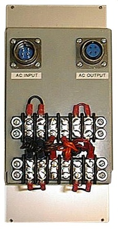
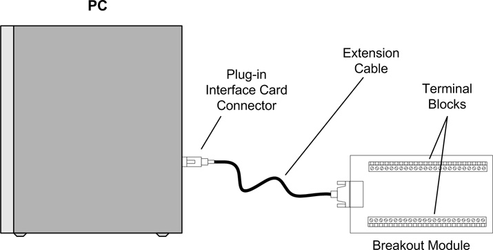
Figure 7-1 shows the business end of a gadget that uses both circular connectors and terminal blocks. We’ll look at both of these types of connectors in just a bit.
DB-Type Connectors
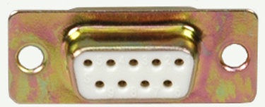
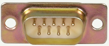
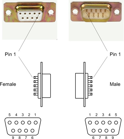
Figure 7-2 shows the female version of a DB-9 connector, and Figure 7-3 shows its male counterpart. These are commonly used for RS-232 interfaces, although they are also used as DC power connectors, RS-485 connectors, and even instrument-specific interface signal connectors.
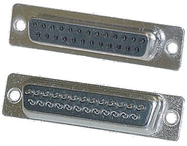
Another commonly encountered connector is the DB-25. It has the same general shape as the DB-9, with the main difference being that it is wider in order to accommodate 25 pins instead of 9. The DB-25 is the connector most commonly used with the full implementation of the RS-232 standard. It is also commonly used for the parallel data printer output port on desktop PCs (and some older notebook/laptop machines). The DB-9 has generally replaced it because it is smaller and not all of the original RS-232 signals are necessary in order to implement a serial interface. Figure 7-4 shows a female DB-25 connector with “solder cup” connections on the back for wiring (more on this in a bit).
Note that all of the DB-type connectors shown so far are panel-mount or shell types. In other words, they are designed to either be mounted in a metal or plastic panel by way of screws through the holes in the flanges on either side of the connector body, or be used with what is called a “backshell,” as shown in Figure 7-5.
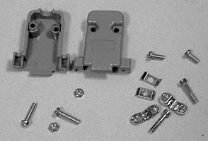
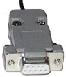
The fully assembled connector looks like the one shown in Figure 7-6.
Both male and female DB-style connectors are available in PCB-mount versions as well. The DB-9 and DB-25 connectors on a PC motherboard connect directly to the circuit traces on the motherboard. As for pin counts, DB-type connectors are also available in 15, 37, and 50 pin types. Finally, several types of high-density D-type connectors are available, such as those used with analog video display monitors. These utilize three or more rows of pins or sockets in the connector body.
Pin numbering for a DB-9 connector is shown in Figure 7-7. Notice that the pins are reversed between the male and female connectors when viewed from the face of the connector.
USB Connectors
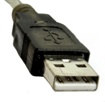
Universal Serial Bus (USB) connector shapes and sizes are defined by the USB standards. They all have four contacts: two for the data signals (D+ and D−) and the other two for power (+5 V) and ground. Typically these are premolded, so (hopefully) you won’t need to assemble any of them. What you should be aware of are the different types of connectors defined by the USB standard.
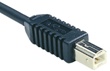
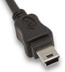
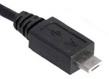
There are four basic USB connector types, as shown in Table 7-1.
Type | Description | |
Type A | Used primarily at the host or controller end of a USB connection. On a PC, these are used to connect keyboards, mice, drawing tablets, cameras, printers, and hubs, among other things. | |
Type B | A square-shaped connector with beveled exterior corners on one side to orient it to a socket. This connector is typically found on external devices such as hubs and printers. | |
Mini USB | This type is commonly found on consumer digital cameras and other mobile devices. | |
Micro USB | Similar to the mini USB but slimmer. The micro USB connector is designed to be more resistant to wear than the mini USB type. |
The instruments we will encounter will generally use the A and B types. It is uncommon to find mini and micro connectors on instrumentation devices. Standards aside, consumer electronics manufacturers have been known to come up with variations of the mini and micro styles that are unique to their products. Even today, many popular MP3 players and cell phones use oddball connectors on the “B” end of what would otherwise be a standard USB cable.
Circular Connectors
Circular connectors are all around us, although they are not always specifically referred to by that name. The “phono”-type connectors on the back of a TV monitor or stereo receiver are examples of single-circuit circular connectors. The BNC connectors used with shielded cable and often found on test equipment and radio gear are another type of circular connector. For professional audio applications, one will find circular connectors with one, two, or four circuits (pins) used for microphone inputs, patch cables, and low-voltage power connections. The 2.5 mm and 3.5 mm stereo-plug-type connectors found on the end of headset or earbud cables are also types of circular connectors, but these are more commonly referred to as “plugs,” which are inserted into “jacks.”
In this book, when the term “circular connector” is used it will refer to the type of connector shown in Figure 7-8.
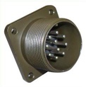
The connector shown in Figure 7-8 is known as a “MIL-type” connector. The reason for this is that these types of connectors were originally intended for military and aerospace applications. As such, they are very robust and can endure harsh environments. Some types, made entirely of plastic, are inexpensive but still relatively robust. Other types, made from aircraft-grade materials and assembled to order by manufacturers with facilities for handling custom orders of various sizes, can be quite expensive (over $200 is not uncommon for a connector built to military standards). Both types are available with pin counts from two to over a hundred.
Figure 7-9 shows the AN/ARC-220. This is a mobile radio system used by the US military that utilizes circular connectors of various types and configurations to interface with an aircraft’s power and avionics systems.
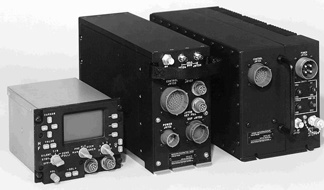
Although you might never encounter the AN/ARC-220 in the wild, it is possible that you might come across some ruggedized instrumentation equipment that looks something like this.
Wiring a MIL-type circular connector involves either soldering the wires into solder cups on the ends on the pins or sockets, or using a special (and typically rather expensive) crimping tool with specially machined pins and sockets. Some of the low-cost multipin circular connectors use stamp-formed pins and sockets rather than solid machined parts, and although they’re not as rugged or reliable, they can be considerably less expensive.
Terminal Blocks
Terminal blocks are ancient (in a technology time sense). They started to appear in common use in the early part of the 20th century, replacing the threaded binding posts and clip-type connectors of the late 19th century. World War II provided a major incentive for the development of more robust and reliable connectors, and the pace of innovation hasn’t slowed since that time.
The name “terminal block” actually refers to a number of different styles of termination devices. A barrier terminal block, like the one shown in Figure 7-10, uses screws to hold down a wire or crimp-on lug-type connector.
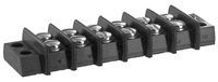
Although one can simply loop bare wire under the screw head, this is not an optimal method. The wire may slip out, especially if it is multistranded. When using bare wire, single-conductor copper wire works best with a barrier-type terminal block. However, because the screw head can create an immobile pressure point where wire flexing is concentrated, there is also a possibility that it will break off. A lug connector is the optimal way to connect a wire to a barrier terminal block. A typical lug connector suitable for use with a barrier-type terminal block is shown in Figure 7-11. You can also see them on the gadget shown in Figure 7-1.
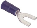
This type of connector does require the use of a crimping tool, but these are common and easily obtainable at any well-stocked hardware store or automotive parts supplier.
A type of compact terminal block more commonly encountered in instrumentation devices is the PCB-mount type shown in Figure 7-12. These are designed to be soldered directly onto a circuit board, and provide a convenient and reliable way to interface with a circuit.
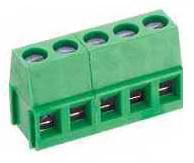
These types of compact connectors are very common in instrumentation devices intended for use with a PC, such as the USB-based interface devices we will examine later. It is also common for interface cards installed in a PC to connect to a module with compact terminal blocks by way of a special multiconductor cable, shown in Figure 7-13.
Wiring a compact terminal block simply involves stripping about 1/4 to 3/16 of an inch of insulation from the end of a wire, inserting the bare wire into the hole below the screw, and then tightening the screw until it clamps the wire firmly in place. No soldering or crimping is required. The downside is that terminal blocks take up more space than some other connector types, and they aren’t always suitable for environments where ruggedness is a primary concern.
Wiring
Wiring a connector correctly the first time can save an immense amount of time, and possibly money, further down the road. As you have probably gathered by now, the two primary means of connecting wires to a connector other than a terminal block are soldering and crimping, and for terminal blocks either a bare wire is inserted into a terminal position or a crimp-on lug is secured under a terminal screw. Regardless of the connector type, there are correct (and incorrect) ways to wire a connector, and we’ll look at a few of them here.
Soldering
If you are new to soldering, it is probably a good idea to get in some practice before tackling a connector. Spending some time with some scrap wires and old circuit boards will pay dividends later. US government publications are an excellent source of information on soldering techniques and standards. For example, NASA STD 8739.3 describes solder connections and contains a wealth of useful information.
Connectors that are designed for solder connections have a special feature called a “solder cup” machined or formed into the end of the pin where the wire is attached. Figure 7-14 shows how NASA defines a good solder cup connection.
Crimping
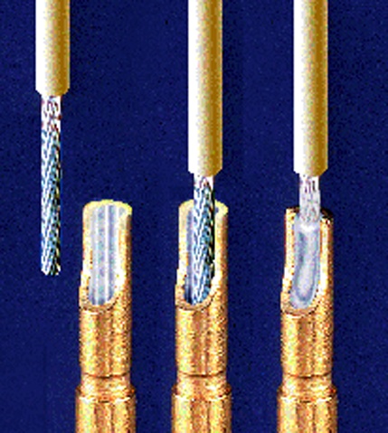
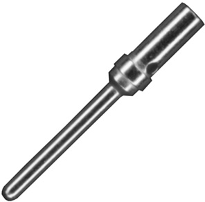
Crimp-type connectors are easier to assemble than solder-cup connections, and for some applications they provide for a more robust connection, but only if the crimp is made according to the manufacturer’s specification using the correct tool. Figure 7-15 shows a machined crimp pin for a circular connector. Once the wire is crimped into the pin it is inserted into the connector from the back using a special tool, where it locks into place within the connector body. It can be removed using another special tool. Of course, for each pin there is a matching socket in the female connector. These are also crimped and inserted into the connector body. Crimped pins and sockets require unique tools that are specifically made for a particular type and size of connector. Crimping tools for MIL-type connectors can cost upwards of $500 (or more) apiece. Other types of crimping tools, such as those used with DB-type connectors or low-cost rectangular connectors such as those made by Molex or Hirose, are usually not as expensive, but nonetheless they still aren’t cheap.
Crimped pins and sockets are inherently strain-relieved by virtue of the design of the crimped part. A crimp-style pin or socket not only “bites” into the bare wire but also has a second area, near the open end of the pin or socket, that clamps down on the wire’s insulation. When assembled correctly and combined with the appropriate backshell, a crimp-style circular or DB-type connector is a very rugged item—which is why you can find a lot of them in aircraft, spacecraft, military field gear, and harsh industrial environments.
Wiring caveats
Here are a few points to keep in mind when wiring a connector:
As a general rule, do not tin the end of a stranded wire when it’s used with a screw-type terminal block. This might seem like a good idea, but it creates a situation that can lead to metal fatigue and broken wires. Leave the wire bare, twist it tightly, and let the screw in the terminal block do its job.
You really want to avoid soldering a wire to a connector that wasn’t originally intended to be soldered. In other words, if a connector uses inserted pins and sockets designed for a crimping tool, attempting to solder a wire to the pin or socket will often result in a connection that is mechanically fragile. It may also turn out to be the case that while a soldered pin or socket can be inserted into a connector body, any stray bits of solder hanging over the sides may jam it in place. It will then be next to impossible to ever remove it should the need arise. This could result in the entire connector ending up in the trash can.
Always use the right wire for the job. Don’t use grossly undersized wire, and don’t try to cram a heavy-gauge wire into a terminal block or lug meant for a smaller gauge. By the same token, if the solder cups on a connector are designed for, say, 18- to 22-gauge wire, trying to solder a 14-gauge wire to it probably won’t allow the wire to seat completely within the cup, and the connection may cause a short with adjacent pins.
Keep things neat. Bundle individual wires with related signals using nylon or plastic cable ties as much as possible. If there are a lot of cable bundles, labeling them can save time and reduce frustration in the future when you have to follow a cable and figure out what each line is supposed to be connected to.
Always use a backshell with connectors on the end of a cable. This goes for circular as well as DB-type connectors. The backshell not only protects the wiring from damage, it also provides essential strain relief. It is common to see DB-type connectors lying around a lab or shop with no backshells. While not assembling the backshell spares you some effort, the odds are good that the wiring on the connector won’t last long if it gets frequent use.
Connector Failures
There are a number of reasons why a connector might fail, and they are all mechanical in one way or another. Bad solder connections, broken or bent pins, loose screws on a terminal block, and broken wires are just some of the possible ways a failure can occur.
As the quote at the start of this chapter states, loose or improperly seated connectors are a major source of problems. If a connector is designed to be used with screws to secure it, use them. If a connector is designed to be locked into place with a threaded or bayonet-type outer shell, by all means use that. Some connectors, such as RCA phono plugs or USB connectors, are designed to be plugged in without any additional hardware to physically secure them, but just plugging in a connector that is meant to be secured and then letting it go at that is an excellent way to increase the odds of experiencing mysterious intermittent failures later.
If a connector is carrying low-level signals, especially in high-impedance circuits, corrosion or dirt can cause the connection to introduce noise into the signal, or cause intermittent failures that mysteriously appear and disappear. Corrosion can occur due to oils and acids from fingertips. Using connectors not intended for harsh environments can also cause problems.
Lastly, you should be aware that connectors are often rated in terms of the number of “insertion cycles” they can tolerate before things become worn and the connection becomes unreliable. Each time a connector is “mated” to its matching part, it counts as an insertion cycle. Some inexpensive DB-type connectors may only be good for around 50 insertion cycles (or less, if they’re really cheap connectors). Other types, such as USB connectors, may have ratings of over 5,000 cycles before the connector starts to experience noticeable wear-related issues.
Serial Interfaces
The three most common types of serial interfaces you are likely to encounter when dealing with instrumentation device interfaces are RS-232, RS-485, and USB. The RS-232 and RS-485 standards were originally given the RS (Recommended Standard) designation by the Electronic Industries Alliance (EIA). When the maintaining organization changed its name the prefix changed as well, first to EIA-232 and finally to TIA-232. The standards are currently revised and maintained by the Telecommunications Industry Association, but since the RS nomenclature is so deeply ingrained in the history of electronics engineering and telecommunications, it has refused to go away. In this book I will use the RS-232 and RS-485 names for these standards.
USB interfaces have become very common over the past decade, to the point where USB has largely supplanted the RS-232 interface once found on just about every PC. Only desktop or rack-mounted PCs still provide serial interfaces (and even some of the thin rack-mount units have done away with them). The latest models of notebooks and so-called netbook computers now have only USB ports.
There are a variety of different types of special-purpose, high-reliability serial interfaces used in specific applications. These include CAN (Controller Area Network), FieldBus, and Profibus. The MIL-STD-1553 serial bus found in military applications and some avionics is yet another example. These are specialized interfaces that are not often encountered outside of limited domains, so we won’t cover them here. However, the basic concepts behind serial communications apply to all serial interfaces, and the RS-485 interface is the underlying framework on which some industrial interfaces are based.
RS-232/EIA-232
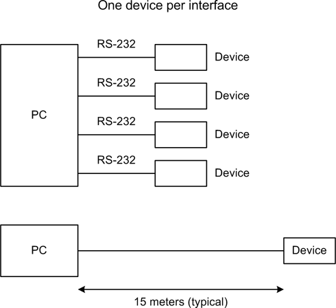
RS-232 is a voltage-based interface; that is, the difference between a logical 0 and a logical 1 is determined by the voltage level present on the signal lines. The standard does not specify the data encoding, only the hardware interface, but it is so closely associated with ASCII character encoding (discussed in detail in Chapter 12) that the two standards have become deeply intertwined. RS-232 has some limitations to be aware of. For example, there cannot be more than one device connected to a single “port” on a PC or other system (usually). In other words, it’s a point-to-point interface, as shown in Figure 7-16. It also has line length and speed limitations because of the use of voltage swings to perform the signaling, and RS-232 tends to be susceptible to noise and interference from the surrounding environment.
RS-232 data formats
As we just mentioned, RS-232 is a voltage-based interface. That is, it uses one voltage level to signify a logical true (1), and another for logical false (0). Figure 7-17 shows how this works.
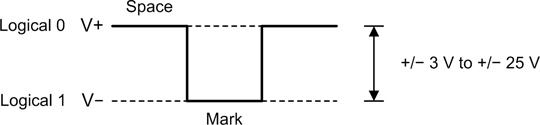
Notice that RS-232 data signals employ negative logic. That is, a logical true (1) is a negative voltage level, and a logical false (0) is a positive level.
When using ASCII encoding, an RS-232 character consists of a start bit (a mark), followed by 5 to 9 data bits, an optional parity bit, and 1 or 2 stop bits (a space). Figure 7-18 shows the format for 8 data bits with no parity and 1 stop bit, and 7 data bits (true ASCII) with even parity and 1 stop bit. In both cases the actual number of bits sent or received for each character or byte is 10 bits. Each unit of data, from the start bit to the stop bit (if used), is referred to as a “frame.”
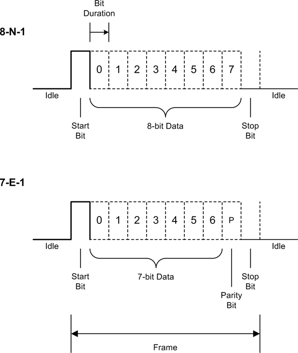
In order for a specific format to work correctly, both ends of the communications channel must be configured correctly from the outset. Attempting to connect a device configured as 8-N-1 to a device set up for 7-E-1 won’t work, even though both ends are sending and receiving 10 bits of data per frame. It will, at best, result in erroneous data at the 8-bit end, and a lot of parity errors at the 7-bit end.
The speed, or data transmission rate, of an RS-232 interface is measured in baud, which is the number of bits per second. What this means is that a serial interface running at 9,600 baud will not send or receive 1,200 bytes or characters per second (9600/8), because at least 2 of the 10 bits in the frame are taken up by the start and stop bits. That is, only 80% of the frame contains actual data. The actual maximum rate just happens to work out to 960 characters per second in this case. As a general rule, if you know the number of bits per data frame, dividing the baud rate by that number will give you the effective rate in characters per second (CPS).
RS-232 signals
The RS-232 interface employs a number of signals for both data transfer and handshaking between two devices. Most of these signals are from the days when RS-232 was first defined and its intended application was to connect a terminal or mainframe to a modem. External modems are becoming scarce, but most RS-232 interfaces still retain the various lines shown in Figure 7-19. Note that these are for a DB-9–type connector; when used with a DB-25 connector there are other signal lines that may be implemented, although they are seldom used.
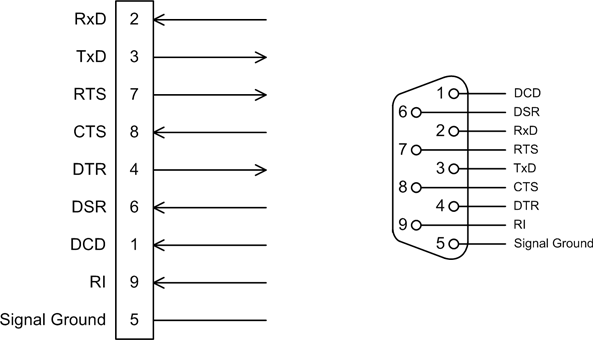
The basic RS-232 signals shown in Figure 7-19 are really all that are necessary to implement a full RS-232 interface with hardware handshaking. The signals are defined in Table 7-2.
Signal | Definition |
RxD | Received Data |
TxD | Transmitted Data |
RTS | Request to Send |
CTS | Clear to Send |
DTR | Data Terminal Ready |
DSR | Data Set Ready |
DCD | Data Carrier Detect |
RI | Ring Indicator |
RS-232 is a full-duplex interface, meaning that data may move in both directions simultaneously. It is also asynchronous, and all data clock synchronization is derived from the incoming data stream itself, not from an additional clock signal line in the interface (there is, of course, an exception to this—RS-232 can be implemented as a synchronous, or clocked, interface—but it is seldom used). RS-232 can also be used in half-duplex mode. See the sidebar Half- and Full-Duplex for more information.
In many cases all one really needs are the RxD (receive) and TxD (transmit) data lines, and some instruments are indeed wired this way. Most instruments with an RS-232 interface will work fine when connected to a PC using the correct cable (typically supplied with the instrument), and no modifications to the interface wiring should be necessary.
DTE and DCE
When working with RS-232 interfaces you will no doubt encounter the acronyms DTE (Data Terminal Equipment) and DCE (Data Communications Equipment). Hailing from the days of mainframes and acoustic coupler modems, these terms were used to define the endpoints and link devices of a serial communications channel. The terms were originally introduced by IBM to describe communications devices and protocols for its mainframe products.
In the context of RS-232, DTE devices are found at the endpoints of a serial data communications channel. The “terminal” in DTE does not refer to a device with a roll of paper and a keyboard (a teletype terminal, or TTY), or a CRT and a keyboard (an old-style computer terminal, or “glass TTY” as they were once known). It literally means “the end.” Figure 7-20 shows this arrangement graphically.
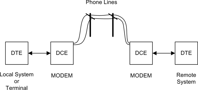
Another way to look at it is in terms of “data sink” and “data source.” A data sink receives data, and a data source emits it. Either end of the channel (the two DTE devices) can be a sink or a source. The DCE devices provide the channel between the endpoints using some type of communications medium. For a system using modems, this would typically be a telephone line.
Nowadays modems are becoming something of an endangered species, although they are still used for data communications in some remote parts of the US and around the world that lack high-speed Internet services. However, the wiring employed in RS-232 cables and connectors still reflects that legacy, which is why it’s important to understand it in order to correctly connect things using RS-232.
The signals described in the previous section are named with reference to the DTE. In other words, on a DTE device, TxD is a data source, or output. On a DCE, it is a sink, or input, for the TxD of the DTE. This also applies to the RxD line. In effect, the DCE’s data source and sink connections are functionally inverted with respect to the DTE’s TxD and RxD lines, even though they have same names. This may seem confusing, but the upshot of it all is that when connecting a DTE to a DCE, the interface is wired pin-to-pin between them (1 to 1, 2 to 2, and so on).
If you need to connect two devices that happen to be DTEs, you will need to use what is called a crossover cable or, if you don’t need the handshake lines, a null-modem cable. Figure 7-21 shows how the TxD and RxD lines would cross over for a DTE-to-DTE interface. It does not show how the handshake lines would need to be connected.
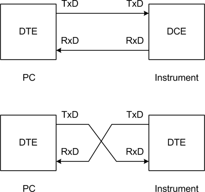
Most devices with a serial port are wired as DTE devices, although some do have the ability to be configured as DCEs. This can be done using jumpers, small PCB-mounted switches, a front-panel control, or even via software. The built-in serial port on a PC is typically implemented as a DTE.
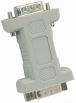
For devices with low-speed interfaces, or when the communications protocol is strictly a command-response format, you probably don’t need the rest of RS-232’s handshaking lines. In this case, you can use a ready-made commercial null-modem cable or a null-modem adapter. Such an adapter is shown in Figure 7-22.
RS-485/EIA-485
RS-485 is commonly found in instrument control interfaces and in industrial settings. Like its predecessor, RS-422, it has a high level of noise immunity, and cable lengths can extend up to 1,200 meters in some cases. RS-485 is also faster than RS-232. It can support data rates of around 35 Mbit/s with a 10-meter cable, and 100 Kbit/s at 1,200 meters.
RS-485 signals
RS-485 owes these capabilities to the use of differential signaling. Instead of using a dedicated wire to carry data in a particular direction, there are two wires that are electrically paired that carry data in either direction, but not at the same time. The two wires in a differential interface are always the opposite of one another in polarity. The state of the lines relative to each other indicates a change from a logic value of “1” to a “0,” or vice versa. Figure 7-23 shows a typical situation involving asynchronous serial data that incorporates a start bit and a stop bit. For comparison, it also shows the digital TTL input that corresponds to the RS-485 signals.
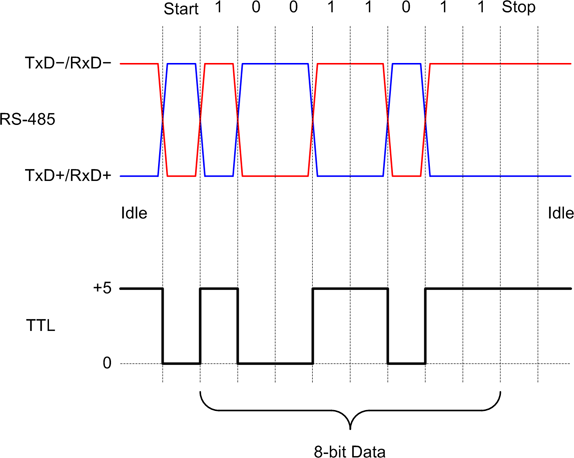
Note that the + and − signals always return to the initial starting state at the completion of the transfer of a byte of data.
Line drivers and receivers
In an RS-485 interface, each connection point uses a pair of devices consisting of a differential transmitter and a differential receiver. This is shown in Figure 7-24.
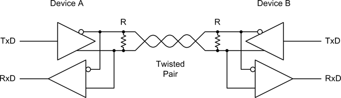
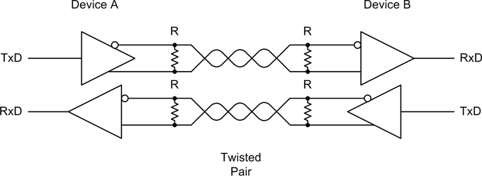
RS-485 may be implemented as a two-wire half-duplex interface or a bidirectional four-wire full-duplex interface, but for many applications full-duplex operation is not required. A four-wire arrangement is shown in Figure 7-25.
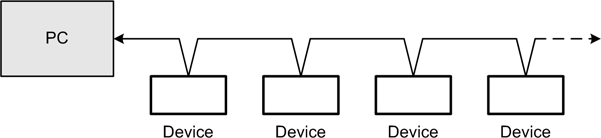
RS-485 multi-drop
RS-485 also allows for more than one device, or node, to be connected to the serial “bus” in what is called a multidrop configuration. This is shown in Figure 7-26. In order to do this, the transmitter (output) section of an RS-485 driver must be capable of being placed into a Hi-Z, or high impedance, mode. This capability is also essential when RS-485 is connected in two-wire mode.
The reason for this is that if the transmitter was always actively connected to the interface it could conflict with another transmitter somewhere along the line. In Figure 7-27 you can see how the drivers take turns being “talkers,” or data sources, when wired in half-duplex mode, depending on the direction in which the data is moving. There is really no need to disconnect the receivers, so they can listen in to the traffic on the interface at any time.
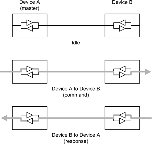
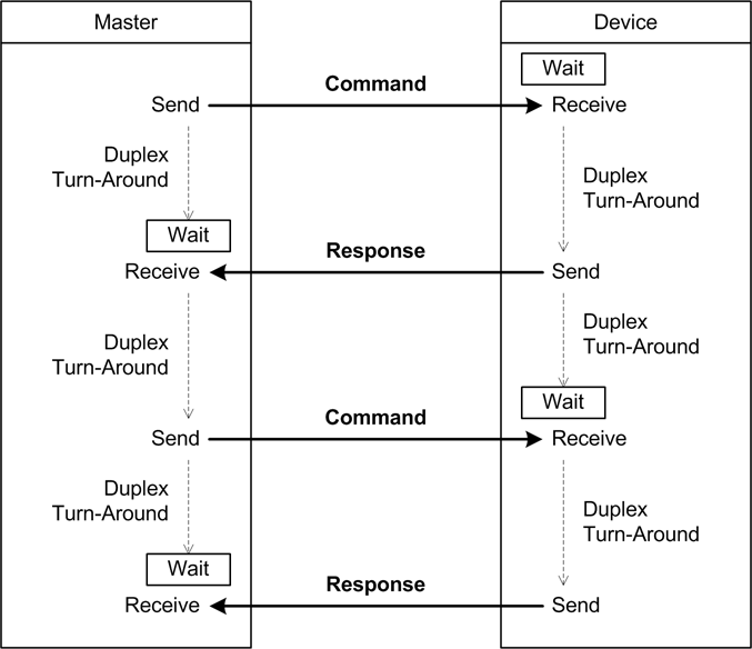
In a typical multidrop configuration, one device is designated as the controller and all other devices on the RS-485 bus are subordinate to it, although it is possible to have multiple controllers on an RS-485 network. The default mode for the controller is transmit, and for the subordinate devices it is receive. They trade places when the controller specifically requests data from one of the subordinate devices. When this occurs, it is called “turn-around.” Figure 7-28 shows how data moves between two devices connected using RS-485 in a two-wire configuration.
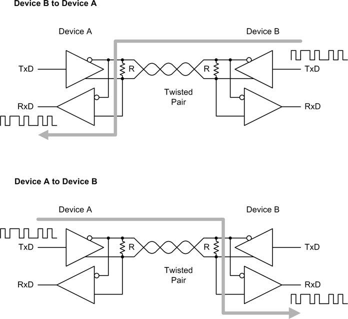
When using a half-duplex RS-485 interface, one must take into account the amount of time required to perform a turn-around of the interface. Even with an interface that can sense a turn-around electronically and automatically change its state from sender to receiver, there is still a small amount of time involved. Some RS-232–to–RS-485 converters can use the RTS line from the RS-232 interface to perform the turn-around as well. Figure 7-29 shows how this works.
Notice that when either device in Figure 7-29 is in the receive mode, there is an explicit wait involved while the device listens for a response from the other end of the channel.
RS-232 versus RS-485
Table 7-3 contains a comparison of some of the electrical characteristics of RS-232 and RS-485.
Characteristic | RS-232 | RS-485 |
Differential | No | Yes |
Max. number of drivers | 1 | 32 |
Max. number of receivers | 1 | 32 |
Modes of operation | Half- and full-duplex | Half- or full-duplex |
Network topology | Point-to-point | Multidrop |
Max. distance | 15 m | 1,200 m |
Max. speed at 12 m | 20 kbit/s | 35 Mbit/s |
Max. speed at 1,200 m | n/a | 100 kbit/s |
In general, RS-232 is fine for applications where there isn’t a need for speed and where the cable lengths are under 5 meters (about 15 feet) or so. Many external instrumentation devices utilize very short (2- to 10-character) commands, return equally short responses, and sometimes take significantly longer to perform the commanded action than the time required to send it from the host system to the instrument. For these types of devices an RS-232 interface at a speed of 9,600 baud is perfectly acceptable. In other cases, such as when one might have sensors or controllers distributed throughout a large system on a single communications bus, RS-485 works quite well. Many manufacturers sell such devices for just this sort of application, and we will look at one in detail in Chapter 14.
USB
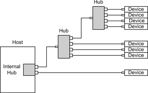
Universal Serial Bus is yet another form of half-duplex asynchronous serial interface. It is similar in some respects to RS-485 in that data is carried as a differential signal on a pair of wires in the USB cable. The cable also includes wires for power and ground. Also, in a USB network only one interface can act as the controller (or host), and all other devices are subordinate.
Figure 7-30 shows a USB network consisting of a host system with an internal hub, two external hubs, and eight USB devices.
For the most part, we don’t need to worry about the low-level details of the USB interface itself. Both the Windows and Linux operating systems incorporate low-level drivers to handle the host chores, and instruments that utilize USB at a low level are provided with software that deals with the communications. In some cases, the vendor may also provide a library module that supports access from user-written application programs. This is more common for Windows than it is for Linux, although some Linux interface drivers are available as well.
USB classes
The USB standard defines various classes of devices that utilize USB interfaces. Some of the more common classes that you might encounter on a regular basis are listed in Table 7-4.
USB class | Example(s) |
Communications | Ethernet adapter, modem |
HID (Human Interface Device) | Keyboard, mouse, etc. |
Imaging | Webcam, scanner |
IrDA | Infrared data link/control |
Mass Storage | Disk drive, SSDD, flash memory stick |
PID (Physical Interface Device) | Force feedback joystick |
Printer | Laser printer, etc. |
Smart Card | Smart card reader |
Test & Measurement (USBTMC) | Test and measurement devices |
Video | Webcam |
You are most likely already familiar with the HID and Mass Storage classes. These two classes include things like keyboards, mice, simple joysticks, outboard USB disk drives, and flash memory sticks (so-called thumbdrives). The HID class is relatively easy to implement, and most operating systems come with generic HID class drivers, so it is not uncommon to find devices implemented using the HID class that don’t look at all like a keyboard or mouse.
If a USB device uses a unique interface (there’s a USB class for this, too), it is up to the vendor to supply the necessary interface drivers, including any low-level drivers needed by the operating system. In cases like this you typically need to install the driver software before attaching the device so that it will be available to the operating system when the new device is detected.
Since we won’t be writing any low-level USB driver software, we won’t delve any deeper into USB classes. The working assumption here is that the device will come with whatever software is needed.
USB data rates
When working with USB devices, it is good to know what to expect of the interface in terms of performance. One potential downside to USB interface devices is speed: many are not particularly fast when compared to what can be achieved using a PCI bus–based interface or a dedicated standalone data acquisition system.
The maximum data rate for a USB interface can vary from 1.5 Mbit/s (megabits/second) to 4 Gbit/s (gigabits/second), depending on the standards compliance level of the interface. The data transfer rates for USB are defined in terms of a revision level of the USB standard. In other words, devices that are compliant with USB 1.1 have a theoretical maximum data rate of 12 Mbit/s in full-speed mode, whereas USB 3.0–compliant devices have a maximum data transfer rate of 4 Gbit/s. Table 7-5 lists the specification levels and the associated maximum data transfer rates.
Version | Release date | Maximum data rate(s) | Rate name | Comments/features added |
1.0 | 1996 | 1.5 Mbit/s | Low speed | Very limited adoption by industry |
12 Mbit/s | Full speed | |||
1.1 | 1998 | 1.5 Mbit/s | Low speed | Version most widely adopted initially |
12 Mbit/s | Full speed | |||
2.0 | 2000 | 480 Mbit/s | High speed | Mini and micro connectors, power management |
3.0 | 2007 | 4 Gbit/s | Super speed | Modified connectors, backward compatible |
USB 3.0 is still rather new, and most USB devices that one will encounter will either be 1.1- or 2.0-compliant. You should also know that even if a device claims to be a USB 2.0 high-speed type, the odds of getting sustained rates of 480 Mbit/s are slim. The time required for the microcontroller in the USB device to receive a command, decode it, perform whatever action is requested, and respond back to the host can be considerably slower than what one might expect from the data transfer rate alone. In addition, the ability of the host controller to manage communications can contribute to slower than theoretical maximum data rates. If the host is busy with other tasks, it may be unable to service the USB channel fast enough to sustain a high data throughput.
How USB devices and hubs are connected can also play a big part in how responsive the communications will be. A USB 1.1 network using 1.1 hubs and devices is only as fast as the slowest device in the network. USB 2.0 hubs deal with this by separating the low/full-speed traffic from the high-speed data. When purchasing new USB components, you should avoid 1.1 hubs and stick to 2.0 units. That way, you can avoid having a high-speed 2.0 device run into a bottleneck due to 1.1 devices on your USB network (assuming that the host controller is itself USB 2.0 high-speed capable).
But speed isn’t everything, and in many instrumentation systems it’s not critical so long as the basic response time requirements are met. Because of the appeal of low cost and ease of use, we will examine various low-cost USB instrumentation devices in the following sections.
USB instrumentation
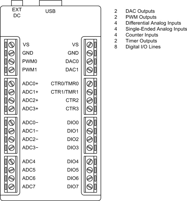
A generic version of the type of USB instrumentation device we can expect to encounter is shown in Figure 7-31. This is similar to several readily available commercial devices and is intended to illustrate the types of inputs and outputs one can expect to find.
Many USB interface devices also incorporate a high degree of internal functionality and configuration options. For example, the hypothetical device shown in Figure 7-31 has discrete I/O lines that may be configured as either inputs or outputs on an individual basis, analog inputs and outputs, and some counter and timer ports. These are typical and are found on many devices of this type. The PWM outputs should be able to accept control parameters to determine the base clock rate and the duty cycle. Some devices may even incorporate the ability to control the duty cycle directly through one of the analog inputs.
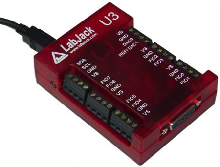
Now let’s look at a real USB interface device. Figure 7-32 shows one type of commercially available USB instrumentation device, the LabJack U3. This is a low-cost (around $110) unit that features configurable discrete I/O; analog input and output channels; timers; counters; and support for SPI, I2C, and asynchronous serial protocols. The U3 employs a full speed (12 Mbit/s) USB interface.
Windows Virtual Serial Ports
Under Windows, one can implement what is known as a virtual serial port (VSP) or virtual COM port (VCP). An aspect of “port redirection,” VSPs have been a part of Windows for quite a long time. A virtual serial port supports most or all of the functionality normally found with any other Windows serial port interface. You can set the baud rate and the number of data bits, and read and write data just as you would with a “real” serial port. The virtual port also emulates the control lines used in a physical serial port, such as RTS, CTS, and so on.
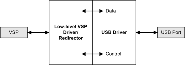
One primary application for a virtual serial port is to provide a common and convenient interface to a physical USB port and the devices that might be connected to it. Figure 7-33 shows a simplified diagram of a VSP-to-USB interface.
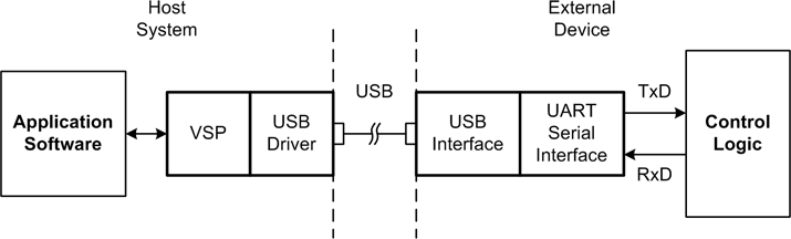
In some cases, a virtual serial port is used with a USB-to-serial converter. USB converters for RS-232 and RS-485 interfaces are readily available, and Figure 7-34 shows a generic diagram of such a device used to interface a serial instrument with a USB port on a PC. ICs from vendors such as FTDI and Silicon Labs are available that incorporate all of the necessary functionality to implement a USB-to-serial interface. With the demise of the RS-232 serial port on the latest computers, particularly notebook and netbook machines, many manufacturers are turning to these types of interfaces for products that would otherwise use RS-232 or RS-485 as their primary control and data interface. In other cases it might serve as the primary connection to an instrument or device that has only a USB interface incorporated into its design, but includes a driver that can translate between serial data and the interface protocol used by the device. The USB-to-GPIB interface we will look at later is one such device.
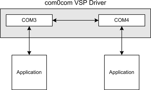
USB redirection is just one application for a virtual serial port and port redirection. A Windows virtual serial port can be used just like a regular serial interface to redirect I/O to another port, or even a network interface. One open source utility that we will see more of later is the com0com package by Vyacheslav Frolov. com0com uses port redirection to implement a pair of virtual serial ports that are connected internally in a default null-modem configuration (although this can be changed when the driver is installed). In other words, writing data to one port will result in the data appearing on the other port. Figure 7-35 shows how com0com does this.
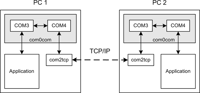
By using a utility called com2tcp (included with com0com) it is possible to link two pairs of virtual serial ports on different PCs via a network connection, as shown in Figure 7-36.
A utility like com0com can be very handy for implementing a real-time monitor and trace facility or a command-line-type user interface, or to simulate an instrument that utilizes a serial interface. The ability to redirect serial interfaces is a powerful tool for working with instrumentation devices.
GPIB/IEEE-488
The General Purpose Interface Bus (GPIB) was developed by Hewlett-Packard in the late 1960s to interface HP test equipment with other test instruments, HP printers, and HP’s line of laboratory minicomputers and mass data storage devices. Originally known as the Hewlett-Packard Interface Bus (HPIB), it was given an IEEE standards designation in 1975.
Although GPIB (HPIB at the time, actually) was used in the late 1970s with some HP computer equipment to interface large external disk drives and line printers, it never really caught on as a data peripheral interface standard. It was, and still is, most commonly found in test and data acquisition equipment.
GPIB/IEEE-488 Signals
GPIB is a type of parallel interface that contains data, command, and interface signal lines in one cable. GPIB addressing allows up to 15 devices to share a single 8-bit parallel data bus. The maximum data rate is around 8 MB/s for the latest versions of the standard.
Internally, GPIB uses 12 lines for various signals and 12 lines for shield and ground connections. Table 7-6 lists the GPIB signals, and Figure 7-37 shows the pin-out of a GPIB connector.
Signal | Pin | Function |
DIO1 | 1 | Data/command |
DIO2 | 2 | Data/command |
DIO3 | 3 | Data/command |
DIO4 | 4 | Data/command |
EOI | 5 | End or identity |
DAV | 6 | Data valid |
NRFD | 7 | Not read for data |
NDAC | 8 | Not data accepted |
IFC | 9 | Interface clear |
SRQ | 10 | Service request |
ATN | 11 | Attention |
Shield | 12 | Cable shield |
DIO5 | 13 | Data/command |
DIO6 | 14 | Data/command |
DIO7 | 15 | Data/command |
DIO8 | 16 | Data/command |
REN | 17 | Remote enable |
Ground | 18 | Ground |
Ground | 19 | Ground |
Ground | 20 | Ground |
Ground | 21 | Ground |
Ground | 22 | Ground |
Ground | 23 | Ground |
Ground | 24 | Ground |
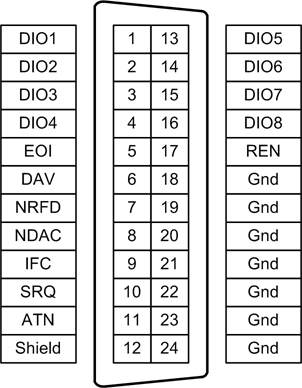
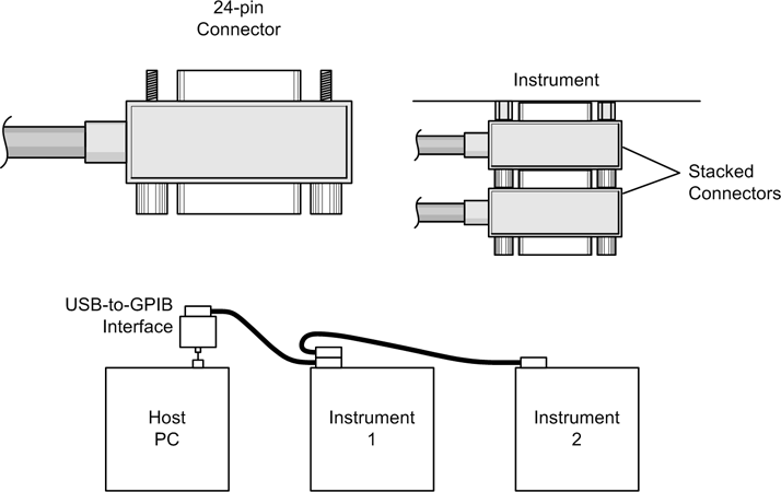
GPIB Connections
GPIB uses a special 24-pin connector that allows connections to be stacked. The slowest device on the bus sets the maximum data transfer rate. Figure 7-38 shows an outline of a GPIB/IEEE-488 connector and how the connectors are stacked to connect two or more devices in a sequential arrangement.
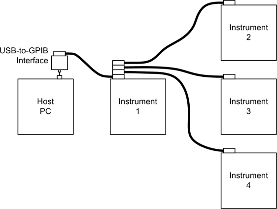
GPIB devices may also be connected in a star configuration, as shown in Figure 7-39.
GPIB via USB
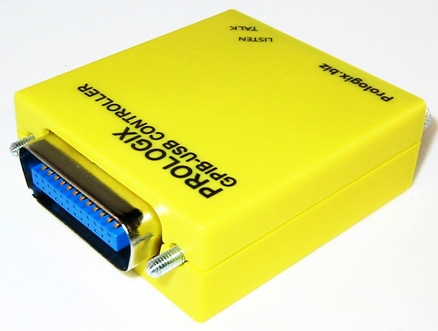
Although one can install a GPIB PCI interface card in a full-sized computer, there are now inexpensive USB-to-GPIB interface modules available. One of these is shown in Figure 7-40. These work well with notebook-class computers, and most include interface software for use with custom applications, as well as drivers with an application program interface (API) for custom software.
The Prologix interface shown in Figure 7-40 uses the FTDI FT245R USB interface chip, and you have a choice of two interface modes: Windows virtual serial port/Linux serial driver, or direct access via a library module. FTDI provides drivers for both Windows and Linux. It is also useful to note that the Prologix device can be connected directly to the GPIB port of an instrument, so one can avoid purchasing a GPIB cable if only one GPIB instrument is involved. It is also possible to equip multiple instruments with their own converters and use a USB hub instead of daisy-chaining GPIB cables between instruments.
Internally, a USB-to-GPIB interface will typically have two main sections: the USB interface hardware and a GPIB interface processor, as shown in Figure 7-41.
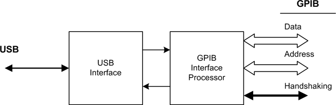
With a USB-to-GPIB converter, you are basically using a serial port (USB) to communicate with a parallel instrumentation bus (GPIB). Internal logic in the converter handles the GPIB handshaking and data transfer operations. If the converter utilizes a virtual serial port, everything that applies to serial programming applies here as well.
PC Bus Interface Hardware
A device designed to connect directly to the internal bus of a computer doesn’t usually have a command-response protocol in the same sense that one would find with the serial or GPIB-type device. Instead, the interface protocol is embodied in the form of callable functions provided by driver software. They are also typically somewhat more difficult to use due to a higher level of software interface complexity.
You can buy various interface cards for a PC that are capable of capturing high-frequency signals in real time, whereas there are no such devices for RS-232 or RS-485, and only a handful with high-speed USB interfaces (and the USB devices often employ some type of buffering, or temporary storage, to help move data between the device and the host system).
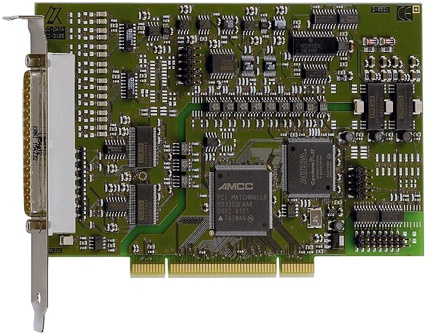
The most common type of bus-based interface cards utilize the industry-standard Peripheral Component Interconnect (PCI) bus and the newest variant, the PCI Express (PCIe) bus. A typical PCI multifunction data acquisition (DAQ) card is shown in Figure 7-42. There are also add-on cards available for the industrial VME bus and the instrumentation PXI bus, but we won’t get into those in this book as most of what we will want to do can be done with PCI- or PCIe-type cards.
Pros and Cons of Bus-Based Interfaces
Bus-based interfaces have a couple of inherent advantages over serial-interface-type devices:
The bus-based interface is always faster than a serial interface, since it has direct access to the internal data bus in the computer. Data can be moved to and from the device in parallel at full (or almost full) bus speed, thereby avoiding the serial interface bottleneck.
The internal settings of the device are directly accessible and the device can generate internal interrupt signals to get the attention of the host system, which makes it possible to incorporate functionality that would otherwise be difficult to build into a device connected using a serial interface.
Figure 7-43 shows the relationship between various types of PCI interface cards and the rest of the host computer system.
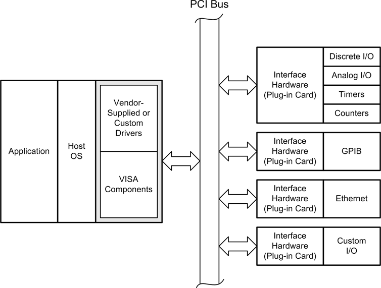
The main thing to notice in Figure 7-43 is that a PCI card always requires additional driver software to interface between the operating system, the application, and the hardware of the interface card itself. A driver will present an API that defines various functions for accessing the interface hardware, such as read, write, set a parameter, return a status value, and so on. We will discuss VISA drivers for instrumentation in Chapter 11.
The driver requirement is one downside to plug-in interface hardware. One cannot just pass ASCII strings back and forth via a serial port. You have to either create software that can interact with the driver’s API, or use the application software provided by the card vendor. The other downside is that the back of a PC can get very crowded very quickly, and some cards use special high-density connectors that are somewhat fragile and must be used with strain-relief brackets so as to prevent them from being pulled or twisted (which can result in a damaged connector, a damaged card, or both). In addition, a PC loaded with interface cards isn’t very portable, whereas a PC that uses serial, USB, or GPIB interfaces can (usually) be unplugged and moved without too much effort.
Data Acquisition Cards
There are numerous types of PCI cards available for data acquisition. Often referred to as DAQ cards, they range in functionality from simple discrete I/O interfaces to complex multifunction devices that almost qualify as computers in their own right.
There are four basic categories of functionality found in PCI data acquisition and control cards. These are listed in Table 7-7.
Function | Description |
Analog output | Multiple analog outputs, typically with 12- or 16-bit resolution. Some models also provide discrete digital I/O capability. |
Analog input | Multiple single- or double-ended (differential) analog inputs at 12- or 16-bit resolution. Eight input channels are common. Some models also provide discrete digital I/O capability. |
Discrete digital I/O | 24 to 96 channel models available, typically TTL-compatible. |
Counter/timer | Provide multiple counter/timer functions (up to 20 counters in some models). Some models also provide discrete digital I/O capability. |
A fifth type, known as a multifunction DAQ card, combines most or all of the four basic functions on one card. These types of PCI cards might include analog inputs (typically 12- or 16-bit resolution), two or more analog outputs, discrete I/O, and counter/timer functions, all under control of logic embedded on the card itself. The PCI card shown in Figure 7-42 is a multifunction DAQ card.
GPIB Interface Cards
Several manufacturers produce PCI GPIB interface cards. These cards are accessed through driver software supplied by the manufacturer, and most provide a programming interface that exposes functions for configuration, addressing, and data exchange.
Given that GPIB has a maximum data throughput of 8 MB/s, or 64 Mbit/s, a GPIB interface running at its theoretical maximum is over five times faster than a full-speed USB interface (but not as fast as a high-speed USB interface at 480 Mbit/s). Consequently, while a full-speed USB-to-GPIB interface may be convenient and easy to use, it becomes less useful as the need for high-speed data transfers over GPIB increases. There are some high-speed USB-to-GPIB interfaces available, but they tend to cost several times what a full-speed device costs.
One example of a plug-in GPIB interface card for the PCI bus is the 82350B from Agilent, shown in Figure 7-44.
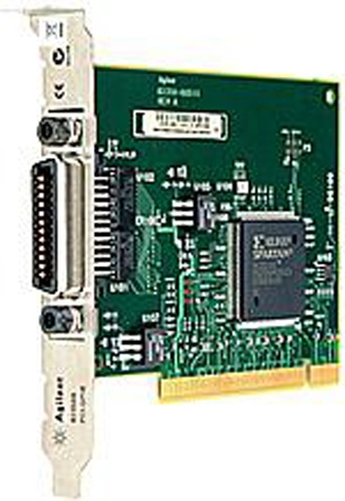
A PCI interface card will often provide features such as buffering for high-speed data transfers and a full suite of IVI standard interface functions.
Old Doesn’t Mean Bad
Just as with used test equipment, there are a lot of used instrumentation and interface devices available. Most of them are still perfectly usable—they’re just not likely to be as fast as newer equipment, or to have the bells and whistles that the newer units offer. Realistically, this shouldn’t matter when you’re working with systems that exhibit changes and responses that take anywhere from seconds to minutes (or even hours). What does matter is how easily the older equipment can be interfaced to a PC, and what kind of software interface it will need.
One downside to the older items is that they usually won’t have any USB support. But that’s really not a big deal in many cases. Unless a device uses a special custom interface, it should still have either a serial or GPIB interface available.
Older devices that employ a custom interface using a plug-in card won’t work with modern computers if the interface card uses an ISA-type bus connection. Other than some models of industrial rack-mount computers, it is simply impossible to buy a new computer with ISA bus slots. Although it is possible to acquire an older PC with a decent CPU and run Python on it, the effort required to assemble the system and then write custom interface software is usually not worth it. It would make more sense to purchase a newer piece of equipment with a more modern type of interface.
That still leaves a lot of older instruments available with serial or GPIB interfaces, and these could well be worth the effort of incorporating them into a system rather than consigning them to the recycler or the landfill. As we will see in Chapter 11, communicating with an external instrument can be readily accomplished with a suitable interface, and the software necessary to achieve this isn’t that difficult to implement.
Summary
We’ve covered a lot of ground in this chapter, and we should now be in a position to actually start thinking about how to select and use the physical interfaces of an instrumentation system. We’ve seen how different connectors are used with different interface types, and we learned the basics of assembling a connector. We then reviewed the various types of interfaces we’ll be dealing with later, from a hardware perspective. We will put this knowledge to good use when we start discussing real instruments and systems in upcoming chapters.
Suggested Reading
While there are some books available on the topics we’ve covered in this chapter, you can probably find everything you need to know on the Web. There is a large amount of information available for RS-232, RS-485, USB, and GPIB. For example:
- http://www.omega.com/techref/pdf/rs-232.pdf
Omega Engineering has made available a compact one-page summary of the RS-232 standard. It’s a handy thing to keep on the workbench or in your lab binder for quick reference.
Also, as you might expect, Wikipedia has entries on all manner of serial communications topics.
Some of the best places to look for technical information on connectors and the specialized tools that go with them can be found on distributors’ websites. Here are a few:
| http://www.DigiKey.com |
| http://www.alliedelec.com |
| http://www.mouser.com |
Federal and military standards are another good resource. Many of these documents go into great detail concerning assembly and interface techniques, and while you probably won’t need all of the information, they also typically include some high-level material, and some even have what can only be described as tutorials. The NASA document referenced here is one such standard, and there are many more available:
- NASA STD 8739.3, “Soldered Electrical Connections.” NASA Technical Standards Program, NASA, 1997.
One of many technical standards freely available from NASA through its Technical Standards Program, this is a concise guide to high-reliability soldering techniques. It is available from http://www.hq.nasa.gov/office/codeq/doctree/87393.htm.
A catalog of available NASA technical standards can be found at http://standards.nasa.gov/documents/nasa.