
Chapter 2. Essential Electronics
Electricity is actually made up of extremely tiny particles called electrons that you cannot see with the naked eye unless you have been drinking.
Although this is a book primarily about instrumentation software, we must also consider what the software is interacting with in the physical world—in other words, the hardware aspects of instrumentation. This chapter is intended to provide a general high-level overview of electricity and basic electronics from an instrumentation perspective, without delving too deeply into the theory and physics behind it all.
Electronics is a deep and vast field of study. Out of a desire to avoid turning this book into a reference work on the subject, some topics are lightly glossed over here, or not even covered at all. If you’re already familiar with electronics at more than just an Ohm’s law level, feel free to skip over this chapter and forge ahead, but if you’re not quite certain what Ohm’s law is, or about the difference between a current source and a current sink, what the term “waveform” means, or how digital and analog input and output differ from one another, this chapter is for you.
We’ll start off with a general description of electric charge and current, and then present some of the symbols used in schematic diagrams. Next, we’ll take a look at very basic DC and AC circuits, followed by a discussion of the types of input and output found in instrumentation systems from an electrical viewpoint. In later chapters, new concepts will be introduced and explained as necessary. We’ll conclude this chapter with a list of references for those who would like to learn more about electronics.
Electrical Charge
For most people, the term “electricity” typically refers to the stuff that one finds in the wires strung along poles beside the street, in a wall outlet, inside a computer, or at the terminals of a battery. But what is it, exactly?
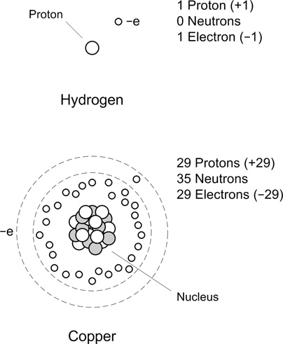
All matter is composed of atoms. Each atom has a nucleus at its core with a net positive charge, and one or more electrons are bound to it, each of which has a negative charge (although one might hear that the electrons “orbit” the nucleus, this is not entirely accurate in the classical sense of an orbit, like, say that of the Earth around the Sun; I would refer you to a modern chemistry or physics text for a better definition than I’m prepared to deliver here). The nucleus of an atom may have one or more protons, each with a positive charge. Most atoms also have a collection of neutrons, which have mass but no charge (one might think of them as ballast for the atom’s nucleus). A typical atom on a typical day in a typical chunk of matter will have a net charge of zero, because there are as many electrons, each with a unit charge of −1, as there are protons in the nucleus, each of which carries a unit charge of +1. Figure 2-1 shows schematic representations of a hydrogen atom and a copper atom.
Some atoms have electrons that are tightly bound, whereas others can lose or gain electrons rather easily. Here’s a simplistic description as to why that is.
In atoms, the electrons are arranged into what are called orbital shells. The outermost shell is called the valence shell. Elements whose atoms have only one or two electrons in the valence shell, and in which the shell is considered to be “incomplete,” tend to release and gain electrons easily. Notice that the copper atom in Figure 2-1 has 29 electrons, one of which is shown outside of the main group of 28. This is copper’s valence electron. Because this electron isn’t very tightly bound, copper doesn’t put up too much of a fuss about passing it around. In other words, copper is a good conductor. An element such as sulfur, on the other hand, does not willingly give up any electrons. Sulfur is rated as one of the least conductive elements, so it’s a good insulator. Silver tops the list as the most conductive element, which explains why it’s considered useful in electronics.
This should be a sufficient model for our purposes, so we won’t pry any further into the inner secrets of atomic structure. What we’re really interested in here is what happens when atoms do pass electrons around, and why they would do that to begin with.
Electric Current
There are two fundamental phenomena involved in electricity: electric charge and electric current. Electric charge is a basic characteristic of matter and is the result of something having too many electrons (negative charge) or too few electrons (positive charge), with regard to what it would otherwise need to be electrically neutral.
A basic characteristic of electric charges is that charges of the same kind repel one another, and opposite charges attract. This is why electrons and protons are bound together in an atom, although they can’t directly combine with each other because of some other fundamental characteristics of atomic particles. The important thing to remember is that a negative charge will repel electrons, and a positive charge will attract them.
Electric charge, in and of itself, is interesting but not particularly useful from an electronics perspective. For our purposes, it’s only when charges are moving that really interesting things begin to happen. Electric current, or current flow, is the flow of electrons through a circuit of some kind. It is also what happens when the static charge you build up walking across a carpet on a cold, dry day is transferred to a doorknob: in effect, the current flows from a high potential (you) to a lower potential (the doorknob), much like water flows down a waterfall. The otherwise uninteresting static charge suddenly becomes very interesting (at least, it gets your attention).
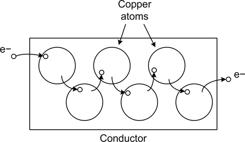
Current flow arises when the atoms that make up the conductors and components of electrical circuits transfer electrons from one to another. Electrons move toward things that are positive, so if one has a small lightbulb attached to a battery with some wires (sometimes known as a flashlight), the electrons move out of the negative terminal of the battery, through the lightbulb, and return back into the positive terminal. Along the way, they cause the filament in the lamp to get white-hot and glow. One way to visualize the current flow is shown in Figure 2-2, where we see a simplified diagram of some copper atoms in a wire. When an electron is introduced into one end of the wire, it causes the first atom to become negatively charged. It now has too many electrons. Assuming that we have a continuous source of electrons with a net negative charge, the new electron cannot exit the way it came in, so it moves to the next available neutral atom. This atom is now negative and has a surplus electron. In order to become neutral again (the preferred state of an atom) it passes its extra electron to the next (neutral) atom, and so on, until an electron appears at the other end of the wire.
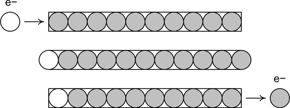
Another way to think about current is shown in Figure 2-3. In this case, we have a tube (a conductor) filled end-to-end with marbles (electrons).
When we push a marble into one end of the tube, a marble falls out the opposite end. The net number of marbles in the tube remains the same. Note that the electrons put into one end of a conductor are not necessarily the ones that come out the other end, as one can see from Figures 2-2 and 2-3.
Basic Circuit Theory
Electricity flows when there is a closed circuit that allows for the electrons to move from a high potential to a lower potential. Stated another way, in order to have current flow we need a source of electrons, and there must be a return point for the electrons. Electric current (a physical phenomenon) is characterized by four fundamental quantities: voltage, current, resistance, and power. We’ll use the simple circuit shown in Figure 2-4 as our baseline for the following discussion.
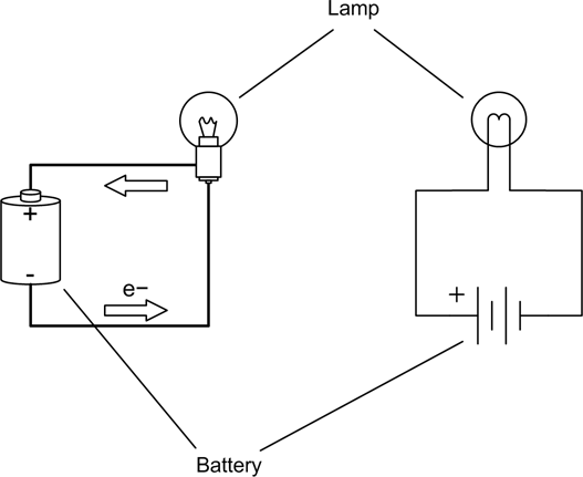
Current that flows in only one direction, as in Figure 2-4, is called direct current (DC). This is what is produced by a common battery, and by the DC power supply in a typical computer system. Current that changes direction repeatedly is called alternating current (AC). This is what comes out of a household wall socket (in the US, for example). It is also the type of current that drives the loudspeakers in a stereo system. The rate at which the current changes direction is called the frequency, and is measured in cycles per second in units of Hertz (abbreviated Hz). So, a 60 Hz signal is composed of a current changing direction at a rate of 60 times per second. We’ll stick to DC circuits for now, and save AC for later.
By convention, current is described as flowing from positive to ground (negative), whereas in reality electrons flow from the negative terminal to the positive terminal of the power source. In Figure 2-4, the arrows show the electron flow. Although you should be aware of this, from this point onward we’ll use the positive-to-negative convention for discussing current flow.
Voltage is the measure of how much electric charge, or electrical potential force, is driving electrons into a circuit. It is measured in units of volts (V). Electric charge is a force, in that a charge will exert a force on other charged objects. How much force is exerted depends on how much charge is present. The concepts of energy, force, and potential are described by classical mechanics, and they also apply to electric charge. The main point to remember here is that a high voltage has more force than a low voltage. This is why you don’t get much more than a barely visible spark from a common flashlight battery at 1.5 volts, like the one shown in Figure 2-4, but lightning, at around 10,000,000 volts (or more!), is able to arc all the way from a cloud to the ground in a brilliant flash. The lightning has more voltage, and hence more force behind it, so it is able to overcome the insulating effects of the surrounding air.
Current is the measure of the volume of electrons moving through a circuit. What the term current means depends on the context. As we’ve been discussing it so far, electric current refers to the flow of electric charge in a conductor, which is a physical phenomenon. In electronics, the word “current” is usually taken to mean the quantity of electrons flowing through a conductor at a specific point at a single instant in time. In this case, it’s referring to a physical quantity and is measured in units of amperes (A or amp).
Resistance is the measure of how much the current flow is impeded in a circuit, and it is measured in ohms. One might think of resistance as an analog of mechanical friction (although the analogy isn’t perfect). When current flows through a resistance there is a drop in voltage across the resistance (as measured at each end), so some of the energy (voltage) in the current flow is being lost as heat. How much energy is lost is a function of how much current is flowing through the resistance and the amount of the voltage drop. As we will see very shortly, there is a famous equation that captures this relationship between voltage, current, and resistance.
Power is the measure of the amount of energy consumed in overcoming the resistance in a circuit or performing work of some sort (perhaps running a motor), and is a function of voltage and current. The common unit of measure is the watt (W), although one will occasionally see electric power expressed in terms of joules (J).
Circuit Schematics
Before moving on, we need to acquire some symbols to help describe what we’re talking about. Electrical circuits are described graphically using diagrams called schematics. There are industry-standard symbols for every type of electrical component available, and how one graphically arranges these describes how the actual components are connected in the physical circuit. Figure 2-5 shows a small sampling of some of the more common symbols one might encounter regularly for what are called “passive” components.
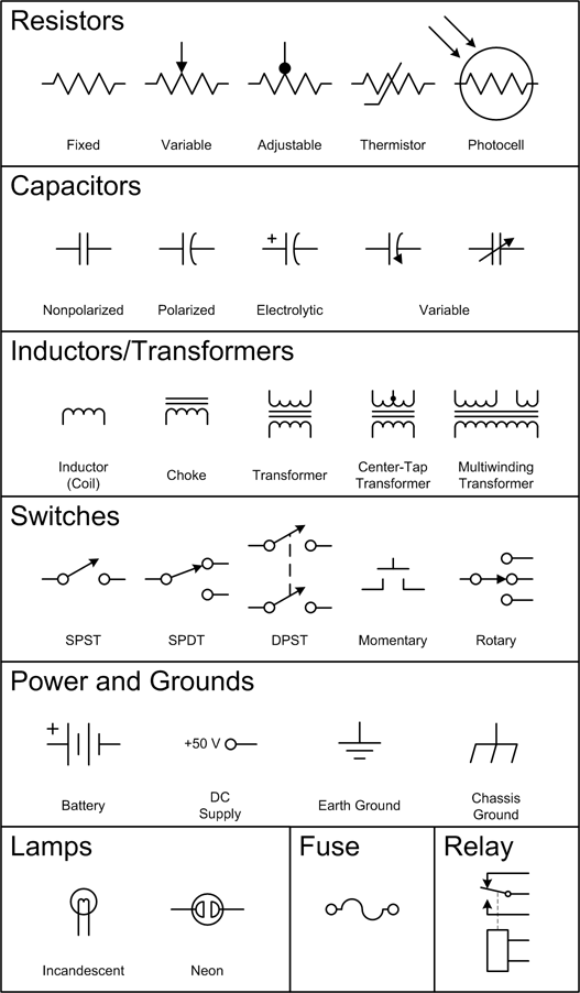
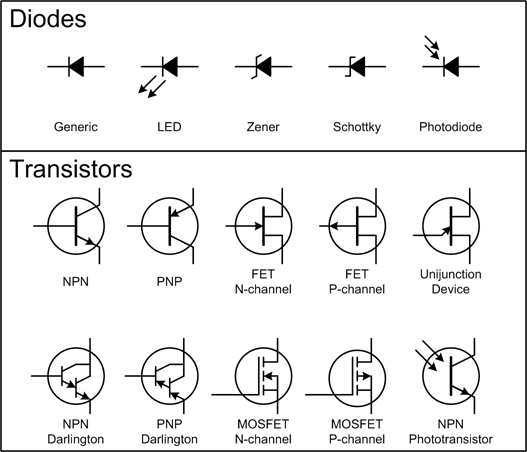
Figure 2-6 shows the symbols for diodes (rectifiers) and transistors of various types. These are referred to as solid-state components and are considered to be active components in that they are capable of altering the current flow in a nonlinear fashion.
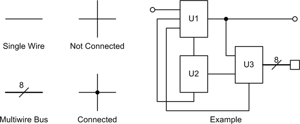
The wires (or circuit board traces) in a real circuit are shown as lines in a schematic. Connections between wires are shown with a solid circle where they meet; otherwise, they simply cross. This is illustrated in Figure 2-7. Some older schematic styles use a small hump in one wire to show that it doesn’t connect to the wire it is crossing, but this has become rather rare in modern diagrams. Also note that in order to avoid drawing multiple parallel lines to represent sets of associated wires, such as digital data buses, the bus is shown as a single heavy line with an indication of the number of individual wires involved.
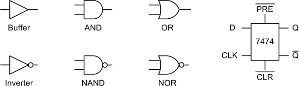
Digital logic has its own set of symbols, and functions within integrated circuits (ICs) such as flip-flops, timers, registers, latches, and so on, are generally shown as rectangles with input and output connections. These types of symbols are shown in Figure 2-8.
The set of schematic symbols presented in Figures 2-5 through 2-8 is by no means complete. A full set of all currently used schematic symbols would be much more involved than what is presented here. In reality, only a small subset of those symbols are necessary for our purposes.
Also, like other specialized fields, electronics is rife with its own peculiar set of abbreviations, acronyms, and other jargon. Here is a small sampling:
- DPDT
A double-pole, double-throw switch.
- DPST
A double-pole, single-throw switch.
- NPN
A type of transistor junction. The acronym refers to the negative-positive-negative “doping” that is used to create the active junctions where modulation of current flow occurs in the device.
- PNP
The opposite of the NPN transistor. It uses positive-negative-positive junctions.
- Polarity
The positive or negative state of a terminal or device.
- Polarized
A device is said to be polarized when it is intended to be used such that one terminal is always more positive (or negative) than the other. Nonpolarized devices are not picky about how they are connected.
- SPDT
A switch with a single pole but two active positions. May also refer to a switch with a mechanical center-off position.
- SPST
A single-pole, single-throw switch.
The small “bubbles” used with digital logic symbols (as shown in Figure 2-8) indicate inversion. That is, if a logical True (1) encounters a bubble, it is inverted and becomes a logical False (0), and vice versa. For example, the truth table for an AND device (where A and B are the inputs) is shown in Table 2-1.
The NAND (Not-AND) device, with a bubble on the output, produces the truth table shown in Table 2-2.
Don’t be confused by the open circles often used to indicate terminal points in a circuit diagram. These do not indicate logical inversion. Only when the open circle is next to a digital component symbol does it mean that logical inversion is applicable.
Schematic symbols will be introduced or revisited as we go along, so there’s no need to commit these to memory at this point. If you’re curious, I encourage you to investigate the references found at the end of this chapter for more details on schematics and the various symbols utilized in creating them.
DC Circuit Characteristics
Now let’s examine the lamp and battery circuit in Figure 2-4 more closely. It may seem simple, but there is actually quite a bit going on here.
When the lamp is connected to the battery, closing the circuit, current will flow through the lamp and then return back to the battery. If it were an open circuit, there would be no current flow and no light (switches are often used to open or close circuits). Generating current flow in a circuit requires a power source capable of producing some volume of electrons (the current) at a voltage (the electrical potential) sufficient to operate the circuit.
When electrical current flows through a circuit, there is always some amount of resistance to the flow; even wires have some resistance. A circuit with low resistance will move current more easily than a circuit with high resistance, and the high-resistance circuit will require a higher voltage to achieve the same level of current flow as the low-resistance circuit. For example, a circuit with a 10-volt supply and 50 ohms of resistance will conduct 0.2 A (also stated as 200 mA, or milliamps—thousandths of an ampere) of current. If the resistance is increased to 100 ohms and we still want to maintain 200 mA of current, the voltage will need to be increased to 20 volts. A high-resistance circuit will also dissipate more power (heat) than a low-resistance circuit at the same current. We’ll have more to say about this a little later.
Ohm’s Law
As you may have already surmised, there is a fundamental relationship between voltage, current, and resistance. This is called Ohm’s law, and it looks like this:
where E is voltage, I is current, and R is resistance. This simple equation is fundamental to electronics, and indeed it is the only equation that one really needs to accomplish many instrumentation implementations.
In Figure 2-4, the circuit has only two components: a battery and a lamp. The lamp composes what is called the “load” in the circuit. Incandescent lamps have a resistance that varies according to temperature, but for our purposes we’ll assume that the lamp has a resistance of 2 ohms when it is glowing brightly. The battery is 1.5 volts, and we’ll assume that it is capable of delivering a maximum current of 500 milliamps for one hour (this is the battery’s total capacity, which is usually around 0.5 amp/hr for a typical AA type battery) at its rated output voltage.
According to Ohm’s law, the amount of current the lamp will draw from the battery is given by:
or:
Here, the value for I can also be written as 750 mA (milliamperes). If we want to know how long the battery will last, we can divide its capacity by the current in the circuit:
This might explain why those cute little single-AA-battery flashlights sometimes handed out at trade shows don’t last very long before a new battery is needed.
In the simple circuit shown in Figure 2-4, the flow of electrons through the filament in the lamp causes it to heat up to the point where it glows brightly (1600 to 2800°C or so). The filament in the lamp gets hot because it has resistance, so current flows less easily through the filament than it does through the wires in the circuit. The power expended to force the current through the filament is expressed as heat. The energy converted and dissipated by a component is defined in terms of dissipated power and is expressed in watts (W). Power in a DC circuit is computed by multiplying the voltage by the current, like so:
If we want to know how much power the lightbulb in our circuit is consuming, we simply multiply the voltage across the bulb by the current:
Now let’s look at a slightly more complicated circuit with some new symbols. Consider the simple LED circuit shown in Figure 2-9. Here we have a resistor in series with an LED (light-emitting diode). There is a 5-volt DC power supply indicated but not shown, and a ground connection (which is the current flow return back to the power supply).
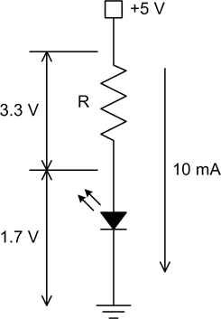
A typical garden-variety red LED device will exhibit a drop of about 1.7 volts across its terminals. Note that this is not the same as the voltage drop across a resistor, but rather a characteristic of the solid-state “junction” that is the heart of the device. If the LED has a nominal rating of 10 milliamps (mA, or 0.01 amps) and we have a 5 V power supply, what size of resistor should we use to get 10 mA through the LED?
Since we can assume a 1.7 V drop for the LED, we can also assume a 3.3 V drop across the resistor. If we solve Ohm’s law for R, we get:
So, a resistor with a value of 330 ohms will supply the 10 mA of current the LED needs to conduct and start glowing. This simple example is more important than you might think, and it will pop up again when we look into connecting LEDs to discrete digital I/O ports later.
Sinking and Sourcing
When reviewing the specifications for an interface device, one may encounter ratings for current sink and source capabilities. What this means, essentially, is that when a load is connected from the device to the positive power source, the device will be able to “sink” up to the specified amount of current before risking damage. Conversely, when the load is connected from the device to ground, it will be able to safely “source” up to the rated amount of current. Figure 2-10 shows this schematically.
The step up and step down symbols indicate how the LED will respond when the voltage from the device is high or low. When the output of the device is low with respect to the +5 V supply the LED in the current sink configuration will be active, and when it is high with respect to ground the LED will be active in the current source arrangement. The same math we used to determine the value of R for Figure 2-9 applies here as well. Note that it is important not to exceed a device’s maximum sink or source ratings. For example, when a device is rated for 20 mA of current source capability, it may mean 20 mA for the whole device, not just for a single output pin.
More About Resistors
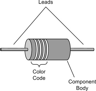
Resistors are ubiquitous in electronic circuits. A resistor can be fabricated from a piece of a poorly conductive carbon material, from a carbon film deposited on a ceramic core, or from a section of resistive wire wound inside a protective package of some type. In addition to a specific resistance value (in ohms), resistors also have a wattage rating. Typical values are 1/10, 1/8, 1/4, 1/2, 1, 2, and 5 watts, with even larger ratings available for special-purpose applications. This sets the maximum amount of power the device can safely dissipate before it risks self-destruction. Lastly, resistors are manufactured to specific tolerances, ranging from 20% to less than 1%, with the price rising as the tolerance tightens. The most common tolerance value is 5%.
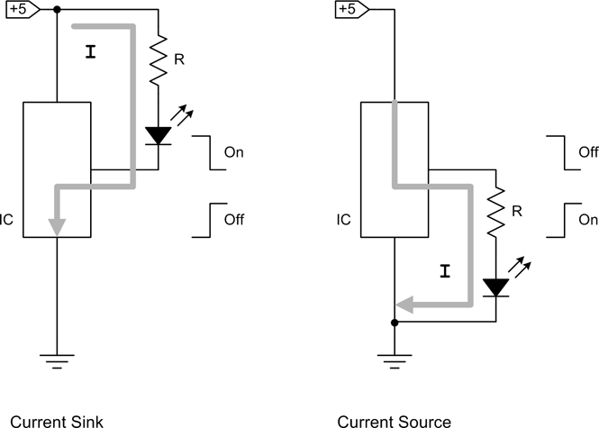
Figure 2-11 shows a generic resistor. Notice that this type of resistor uses color bands to denote its value. You can find the resistor color code in any basic electronics text, and it is explained on numerous websites, so we won’t go into it here.
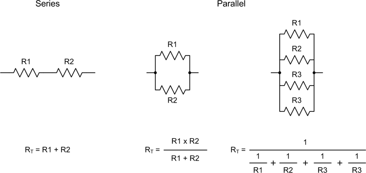
Resistors can be used to reduce a voltage level or limit the current in a circuit, among other things. Resistors are often found in instrumentation applications in circuits such as the one in Figure 2-9, in the role of current limiter. Resistors can be used singly, or they can be connected in parallel or serial configurations. Figure 2-12 shows both, and the simple math used to calculate the equivalent resistances.
We now have enough pieces of the DC puzzle to start to do useful and interesting things with voltage, current, and resistance. Figure 2-13 shows a simple arrangement of two resistors called a voltage divider. These appear quite frequently in electronic circuits.
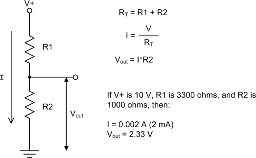
The math necessary to determine the voltage across R2 in Figure 2-13 is straightforward. Once you know the total resistance, you can find the current, and since the current through both resistors is the same it then becomes a simple matter of applying E = IR to find Vout.
AC Circuits
As mentioned earlier, current flow that changes direction over time is called alternating current, or AC. AC is a bit more complex than DC. As well as the expected characteristics of voltage and current, it has the additional characteristics of frequency and phase.
When talking about the power wiring in a house, for example, one would expect to hear terms such as “AC,” “AC voltage,” or “AC current” (which is somewhat redundant). These terms typically refer to the electrical power type in general, the voltage in the circuit, and the current in the circuit, respectively. However, when referring to the low-voltage, low-current AC typically found in instrumentation circuits, the common term is just “signal” or “AC signal.”
Sine Waves
AC signals can occur with any one of a number of types of waveforms, but the sine wave is the prototypical AC signal. A sine wave is “pure”; that is, it is composed of just one frequency. Other waveforms can be decomposed into a series of sine waves by means of Fourier analysis techniques (which we won’t delve into here), but a pure sine wave cannot be decomposed any further.
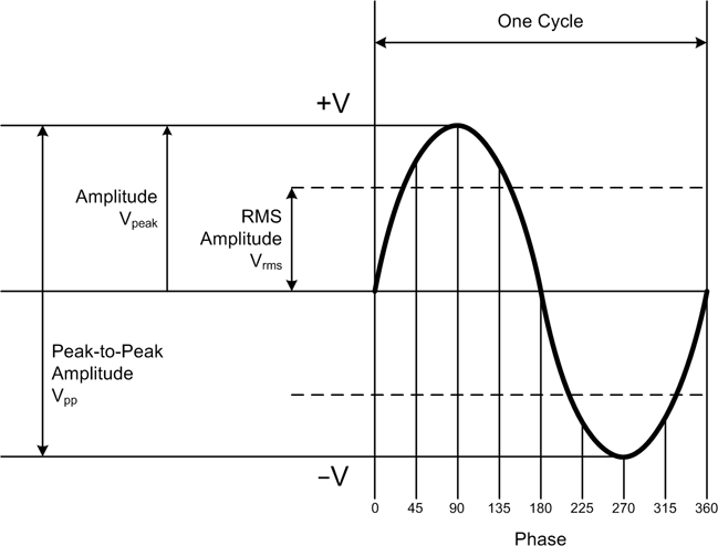
A generic sine wave is shown in Figure 2-14. The sine wave gets its name because mathematically it is defined by the sine function:
where A is the amplitude, f is the frequency, t is time, and θ is the phase. Sometimes one might see this form:
where ω, the angular frequency, is actually just 2πf.
A fundamental characteristic of an AC signal is its frequency. Frequency is the measure of the number of times the signal changes direction (that is, changes polarity) in one second of time and is measured in units of Hertz (Hz). The inverse of a signal’s frequency (f) is its period (t), which is the time interval between each repetition of the waveform:
For example, if a video camera generates frames at a rate of 30 ms (milliseconds) per frame, it is operating at a frequency of 33.33 Hz. The time period of a 60 Hz signal is about 16.67 ms. A signal with a frequency of 10 KHz (kilohertz) has a time period of 100 μs (microseconds, often written as u instead of μ).
Another essential characteristic is amplitude. There are three ways to describe the amplitude of an AC signal: peak amplitude, peak-to-peak amplitude, and root-mean-square (RMS) amplitude. Take a look at Figure 2-14 again and notice that the peak value (the A in the sine wave equations) refers to the maximum value on either side of the zero line. When we talk about the peak-to-peak value (written as Vpp), we are referring to the range between the positive peak and negative peak. Lastly, the RMS amplitude is used to compute power (measured in watts, as with DC circuits) in an AC circuit. For a sine wave Vrms = 0.707 * Vpeak, and for other waveforms it will be a different value.
Now, here’s something to consider: the AC power in your house is probably something like 120 VAC (volts AC). That is its RMS value. The Vpeak value is around 165 volts, and the Vpp value is about 330 volts. The Vpp value isn’t really something to get excited about, but it might be useful to know that the actual Vpeak value is 165 volts when selecting components for use with an AC power circuit. Just remember that the RMS value of 120 VAC is used primarily to compute power.
Capacitors
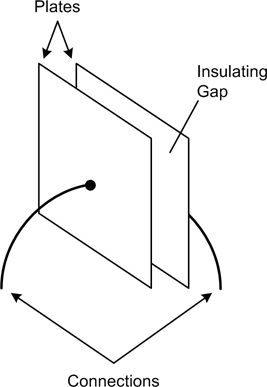
A capacitor is a passive component that is basically two parallel plates with a small gap between them. They come in a wide variety of materials, values, ratings, and sizes. Some capacitors are built using thin layers of aluminum as the conductive plates with an equally thin layer of insulting material between the layers; other types use a porous material soaked in an electrolytic solution as the separator between the conductors, and some incorporate a piece of ceramic material with metalized surfaces on opposite sides. Figure 2-15 shows a generalized view of a capacitor.
Units of capacitance are measured in farads (F, named after Michael Faraday). In electronics applications one will typically encounter values ranging from tens of picofarads (pF, 10−12 F) to upward of several hundred microfarads (μF, 10−6 F). Values measured in whole farads are also available for specialized applications.
Capacitors are a type of charge storage device, similar in many ways to the Leyden jar used to store electrostatic charges (the Leyden jar was invented around 1745 and named after Leyden University in the Netherlands). In a capacitor, the area of the plates and the size and type of the gap determine the capacitance of the device. The larger the plates, the more charge they can hold, and the distance between them determines how effectively the charges on the plates can interact. Capacitors can be fabricated using nothing more than metal plates separated by air: versions of this scheme with movable plates were once common in the tuning circuits of radio equipment and are still in use today. Most small capacitors found in electronic circuits use a dielectric (insulating) material that allows the plates to be very close without actually creating a directly conducting path.
When a voltage is applied to a capacitor, one of the plates will become charged in one polarity, while the other plate will take on the opposite polarity. This is illustrated in Figure 2-16.
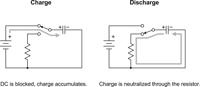
When the switch in Figure 2-16 is set to the opposite position, the capacitor will discharge the energy it accumulated through the resistor. As one might surmise, one way to view a capacitor is as a type of short-term battery (in fact, the term “battery” was coined by Benjamin Franklin to describe an array of the Leyden jars mentioned earlier). Interestingly, there are now available capacitors with values measured in terms of whole farads that are capable of holding a large amount of charge for long enough to actually take on the role of a battery in some applications.
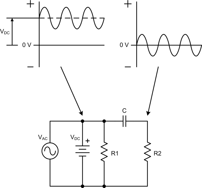
A capacitor will block DC but will pass AC. How well a capacitor will allow the AC signal to pass is a function of the capacitance value, any associated resistances in the circuit, and the frequency of the AC signal. In Figure 2-17, we have a circuit that combines an AC voltage source with a DC voltage source (a battery, for instance).
We can see a couple of interesting things immediately in this figure. The first is that AC and DC can exist simultaneously on the same wire (this is actually quite common in electronic circuits). Secondly, the AC signal will “ride” on top of the DC voltage, with the zero-crossing level of the AC signal at the maximum VDC level. This is often referred as a DC offset or a DC bias, depending on the context.
Notice in Figure 2-17 that one can measure the composite AC-DC signal across R1, but the capacitor C will block the DC and allow only the AC to pass, so taking a measurement across R2 shows only the AC signal. Actually, we’ve neglected to consider the interaction between the resistors and the capacitor, which will affect how the circuit will respond to different signal frequencies. In other words, this is a type of passive filter.
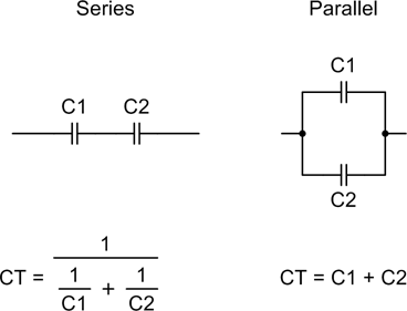
Like resistors, capacitors can be combined in series and in parallel, although the math involved is a little different. Figure 2-18 shows how to compute the equivalent capacitance for series or parallel arrangements of capacitors.
The ability of a capacitor to block DC can be put to use in a variety of interesting ways in instrumentation systems. Consider the situation where one might have an electromagnetic tachometer for measuring the revolutions per minute (RPM) of a rotating device. If the signal suddenly stops, how can one know if the tachometer failed, the circuitry failed, or the mechanism came to a sudden stop without actually going and looking? Figure 2-19 shows one way to do this.
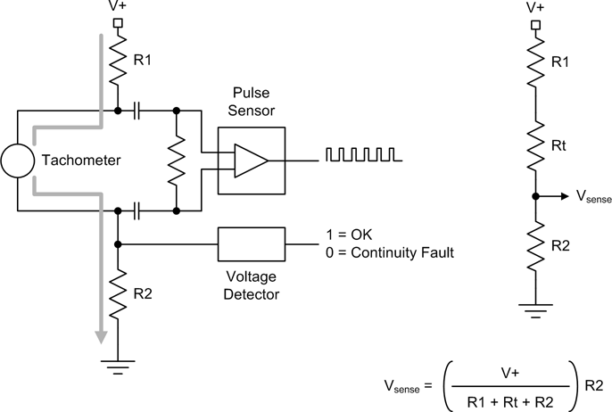
In Figure 2-19 the circuit to the right is the equivalent DC circuit, where Rt is the DC resistance of the tachometer itself. This would probably be on the order of only a few ohms. The capacitors block the DC, and R1, R2, and Rt form a voltage divider. If the tachometer should fail and open the circuit, the voltage detector will indicate the fault when its input goes to zero. Conversely, if the voltage suddenly goes up, the tachometer is probably shorted. Lastly, if the signal ceases but the continuity through R1, R2, and Rt is still good, either the pulse sensor circuit has failed or there is a mechanical problem (i.e., something isn’t moving).
Inductors
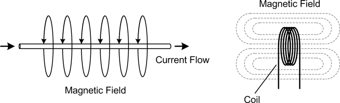
Electricity and magnetism are closely related (exactly how is still not fully understood). Current flow through a conductor will create a magnetic field, and a magnetic field in motion will induce current flow in a conductor in response. Consequently, when current flows through a conductor an associated magnetic field is generated around the conductor, as shown in Figure 2-20. If the current is DC, the magnetic field remains static until the current flow stops, at which point it collapses. When a magnetic field collapses it creates a current flow in the direction opposite to that which created it in the first place (the collapsing magnetic field is in motion). When the wire is wound into a coil, the magnetic field is concentrated. The use of an iron core further increases the effect.
When a coil is energized with DC the result might be an electromagnet, although AC electromagnets are also common. Electromagnets can be found in relays, solenoids, and electric motors.
When a coil is used to alter the behavior of a circuit, it can have the interesting effect of presenting a variable amount of impedance to an AC signal that depends on the frequency of the signal. The only effect a coil will have on a DC signal (other than the creation and collapse of the magnetic field) is the basic resistance of the wire used to wind the coil.
The frequency-dependent response of a coil (also called an inductor) to an AC signal is referred to as the inductance of the coil, and it is measured in henries (H, named after Joseph Henry). In electronic circuits, the millihenry (mH) is the unit most commonly encountered.
From the preceding description it follows that a simple length of wire is an inductor, particularly at high frequencies. This effect can degrade signals traveling over long distances, such as pulses or square waves.
In a DC circuit an inductor is basically a short (or a very, very low resistance), so it isn’t all that interesting. However, in an AC circuit an inductor will impede AC (hence the term impedance) by generating a reverse current each time the signal goes from a peak amplitude (either negative or positive) back toward zero. The amount of the impedance is a function of the inductance of the coil and the frequency of the AC signal.
We won’t go into the details of inductive circuits in this book, although the topic is by no means any less important than any other aspect of circuit theory. In general, we won’t really need to worry too much about it, and when the need arises we will deal with it. The interested (or curious) reader should check out the references at the end of this chapter for more information.
Just as current flow creates an associated magnetic field, a moving magnetic field can generate current flow. Whenever a conductor intersects magnetic lines of force, a current flow will occur. This is shown in Figure 2-21 in the form of a simplified AC generator, also known as an alternator.
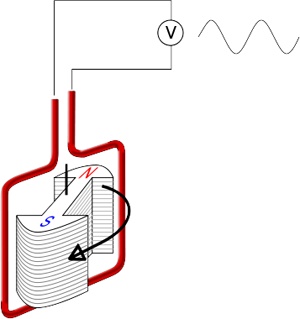
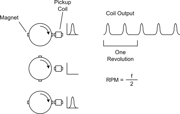
In Figure 2-21, an AC voltage is induced in the wire as the magnet rotates. One could also arrange the device such that the coil rotated through a stationary magnetic field. The end result would be the same. This effect has some useful applications in instrumentation, particularly when one wants to measure the rate of rotation of some mechanism. Figure 2-22 shows the basic idea behind an electromagnetic tachometer.
The output from the coil is idealized here, and in reality it may look quite a bit different. The idea, however, is the same: as the magnets pass the coil a voltage pulse or spike will be produced. Two magnets are shown here because one would usually want things to be balanced on a rotating device or shaft, especially if the mechanism spins at high revolutions per minute (RPMs). Because there are two magnets, every two output pulses represent one revolution of the mechanism.
Other Waveforms: Square, Ramp, Triangle, Pulse
Besides sine waves, there are other waveforms commonly found in electronic circuits. The basic shapes are shown in Figure 2-23.
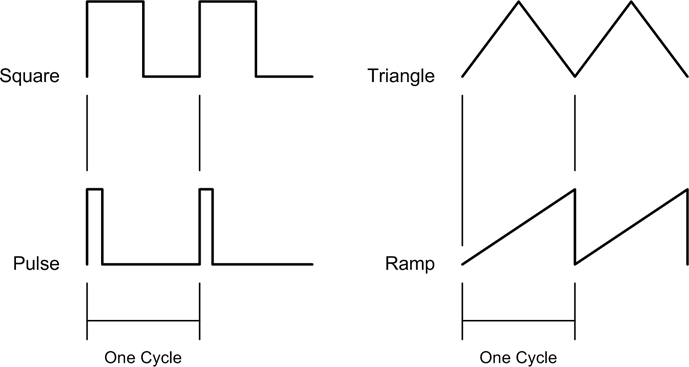
There are, of course, very complex waveforms, such as those found in audio signals. The complexity arises because an audio signal can contain many components with different frequencies. We’ll focus on the types of waveforms one is most likely to encounter in instrumentation circuits.
One of the most common (and most useful) of the nonsinusoidal waveforms is the square wave, together with its close relative, the pulse. Although a square wave is usually drawn with a shape that implies instantaneous on and off times, in reality square waves tend to be rather messy. This is shown in Figure 2-24.
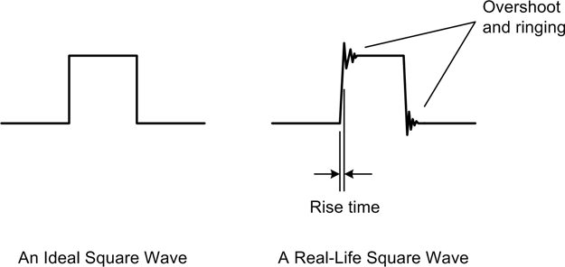
The overshoot and ringing occur because of the various impedance and capacitance effects in a circuit. Because a wire has intrinsic inductance (as was stated earlier), sending a pulse or square wave over more than a few feet of unshielded wire will result in a degraded signal at the receiving end. There are ways to get around this, or at least reduce the effect, as we’ll see later.
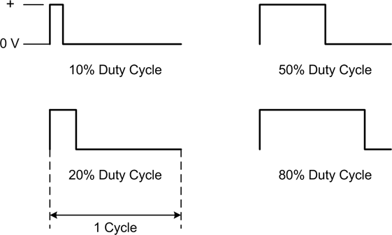
When dealing with pulses and square waves, one often refers to the duty cycle of the waveform. In fact, a square wave is actually a pulse with a 50% duty cycle. That is to say that it is on for one-half of a cycle. Figure 2-25 shows some pulses at various duty cycles.
Interfaces
In an instrumentation system, the interfaces are where the software meets the real world. An interface might be as simple as an input to sense the open or closed state of a switch, the voltage from a temperature sensor, or pulses from a magnetic sensor on a rotating shaft. An interface can also be a data communications channel for interfacing with a self-contained instrument or controller of some type. It could even be another computer system, as in the case of an Ethernet interface.
Discrete Digital I/O
A discrete digital interface gets it name from how the input and output bits, also called lines or pins, are organized, read, and controlled. Discrete digital I/O can be used whenever there is a need for sensing discrete input states or controlling something with discrete operational states. “Discrete” in this case means that each input or output line has a finite number of unique discontinuous states. With a discrete digital interface, this equates to two states: on or off, 1 or 0. Discrete I/O lines may be handled in software as either singular bit values or members of a set of bits. In some cases, a particular line may be configured as either an input or an output. In other cases, an interface may provide a set of lines dedicated to output, and another set for input. As for terminology, it is common to hear “discrete I/O” or “discrete line.” The digital part is understood.
Discrete I/O lines are often grouped in multiples of eight, which is the size of an 8-bit byte, but one can build interfaces with almost any number of discrete I/O lines (at least within practical limits). When a discrete interface is grouped by eight, each set of eight lines may compose what is referred to as a port.
There are quite a lot of indefinites in the preceding sentences, because how an interface is organized is entirely up the engineers who designed it. But from the viewpoint of a microcontroller device, the use of ports containing eight discrete lines is a natural extension of the microcontroller’s internal architecture. Figure 2-26 shows how an 8-bit discrete I/O port could be implemented. Prior to the advent of low-cost microcontrollers and programmable logic devices this was a common way to implement such an interface, and it is still used today.
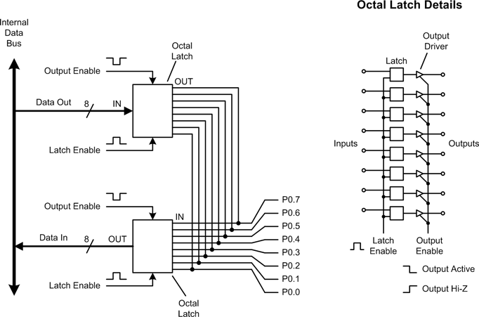
In Figure 2-26, there are two groups of eight signals (1 byte’s worth) connected to each octal output latch device (octal means eight), and another set of eight coming out of the octal input latch device. In other words, this interface will read or write 8 bits of data, or 1 byte, at a time. These are internal data buses, and they would most likely be connected to a main data bus at some point. The various signals shown going into the output and input latches are used to control when the latch should sample the input data (the latch enable signals) and when it should actually make the data available on its outputs (the output enable signals). When the outputs on either latch are not enabled they are in a high-impedance (Hi-Z) state, which is effectively an open circuit. This allows the interface to be either an input or an output, but it cannot be both at the same time. It would not make any sense to set an output line to a high level while trying to read the input from an external device, which might be low. Even if nothing overheated, it still would be a pointless thing to do. However, in the circuit shown in Figure 2-26 it would be possible to write data to the output lines and then read the data back. This is sometimes done to verify that a short to ground does not exist on any of the I/O lines.
Some interface devices, and some microcontrollers, provide the ability to assign discrete I/O pins as either inputs or outputs on an individual basis. In this case the I/O lines would be addressed in the software individually, rather than as a group of 8 bits. Assuming that the interface circuit had this capability, one could use something like the line names P0.0, P0.1, and so on, in the software to refer to specific pins (in this case, specific pins, or lines, on port 0).
It is common for a discrete interface to utilize standard transistor-transistor logic (TTL) voltage levels, although other voltage levels are sometimes used. With TTL, anything below 0.8 volts is considered to be a zero, and anything from 2.0 volts to Vcc (assuming the DC supply voltage is 5 volts) is a logical one. The range between 0.8 and 2.0 volts is invalid. In order to ensure that the input levels don’t wander into the invalid range resistors are often used to either pull the input up, or pull it down. This is shown in Figure 2-27.
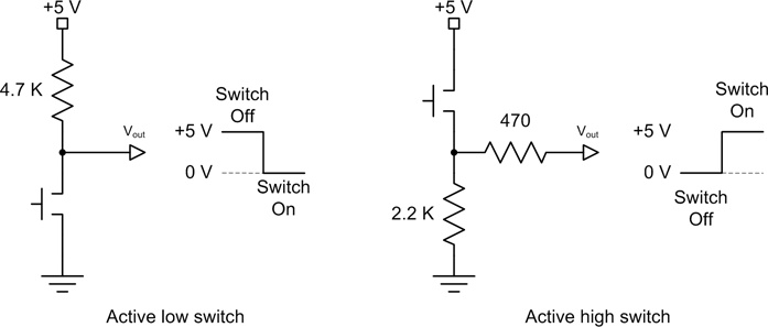
In Figure 2-27, the push-button switch will cause Vout to go to zero when the switch is closed. The 4700-ohm resistor (shown as 4.7 K) will conduct slightly more than 1 mA when the switch is closed, which is negligible in most cases. More importantly, it will provide a constant source of voltage to a digital input, thereby holding it in the logic 1 state until the switch is closed and Vout is pulled to ground (the switch effectively being a short). The active high switch circuit does the inverse, although here we’re trying to hold Vout low until the switch is closed. When the switch is open, the digital input connected to Vout is pulled to ground through the two resistors. When the switch is closed, +5 V is applied to the input through the 470-ohm resistor and a logic 1 is sensed. The 470-ohm resistor limits the amount of current applied to the digital input to about 11 mA. While this resistor may not be absolutely necessary, it is still a good idea. Otherwise, the entire current capacity of the power supply, which may be many amperes, is present at the input of whatever the circuit is connected to. About 2 mA of current will flow through the 2200-ohm resistor when the switch is closed.
When using a mechanical switch as an input you should always keep in mind that switches have a tendency to exhibit what is called contact bounce, or contact chatter. In other words, the contact closure is seldom a clean, snap-on type of thing. Instead, the contacts inside the switch will tend to bounce off of each other for a little while after the switch is closed. This can result in a situation where a switch will generate a series of short on-off events before it finally settles down into one state or the other. Typically this occurs over an interval ranging from just a few milliseconds to upwards of 100 ms or so, depending on the type of switch involved. To avoid reacting to contact bounce the input is “debounced,” either using logic or in software.
The switches in Figure 2-27 could just as easily be limit switches on a moving part, or optical sensors detecting objects passing by on a conveyor, or even float switches in a vat or beaker. A pull-up resistor is also useful for helping to reduce signal degradation over a length of wire by making the sender actively pull the signal low, and otherwise holding it high, as shown in Figure 2-28. This helps to prevent the introduction of noise and also helps make the high to low and low to high voltage transitions more definite (i.e., the signal will have less tendency to “float” or drift between the high and low states).
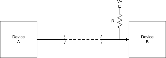
The value of R will largely depend on what type of output circuit device A happens to have. Some logic devices have what is called an open-collector output, which is intended to be used with an external pull-up resistor. Other devices do not have an open-collector output but can still be used with an external pull-up, provided that the value of R does not result in the device sinking more current than it is rated for.
We’ve already seen how a discrete digital output line can be used to directly control an LED (recall Figure 2-9), but they can also control other interesting things if the right type of interface circuit is used. Applications include relays for switching large amounts of voltage or current, solenoid valves, mechanical actuators, or electric brakes, to name but a few.
Figure 2-29 shows how one might arrange for a discrete output to drive a relay. Normally a discrete output is only capable of sourcing a small amount of current, on the order of 10 to 20 mA, and a relay might require significantly more. Connecting a relay directly to the output would result either in no operation or a damaged discrete I/O interface, or both.
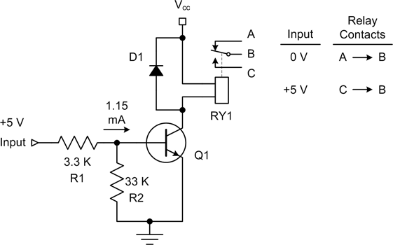
In Figure 2-29, an NPN transistor is used as a current switch. It doesn’t really matter what type of NPN transistor is used for a circuit like this, so long as it is what is called a “small signal” type and it can handle the current through the relay coil. A 2N2222A is a typical choice for small, low-power relays. When the base terminal of the transistor is positive (the “P” part of NPN), the transistor will conduct, and it is capable of handling much more current than the discrete interface alone. R1 and R2 form a voltage divider, supplying around 4.5 V or so at about 1.15 mA to the input (the base) of the transistor when 5 V is present on the input terminal. When there is no input voltage, R2 acts as a pull-down to hold the transistor in an off state. R1 is a current limiter to provide enough current to drive the transistor but not so much as to damage it. Diode D1 is used to prevent the relay coil from sending a reverse voltage spike back into the transistor, which will almost certainly destroy it (recall from our earlier look at inductors that when current through an inductor is removed it will generate a reverse current flow as the magnetic field collapses). Now we have a circuit that can control a significant amount of current by means of the relay contacts. This same circuit could be used to drive a variety of high-current loads.
To avoid having to build such a circuit, one can purchase ready-made relay driver modules and use them with discrete outputs. This is the approach I would advocate, but it definitely doesn’t hurt to have some idea of how the modules work.
Analog I/O
Analog data is converted into digital values using a device called an analog-to-digital converter (ADC). Conversely, a device called a digital-to-analog converter (DAC) is used to convert a digital value into an analog voltage or current. These functions were once quite expensive, and the necessary hardware occupied many circuit boards and a lot of cabinet space. Nowadays, many low-cost microcontrollers have ADC and DAC functions built into the chip itself. The voltage ranges and resolutions of these devices vary widely; for some applications it makes more sense to use an external high-resolution device capable of operating at high conversion rates, but even these are not excessively expensive.
Analog data is problematic for a computer. Because of the discrete digital nature of a computer, it is simply not possible to capture analog data and convert it into a digital form with a level of accuracy that will allow for a 100% faithful representation of the original signal. The same applies to converting digital data into an analog signal. This effect is called quantization, and it arises as a consequence of obtaining or generating a sequence of measurements of a continuously variable signal at discrete points in time.
Acquiring analog data
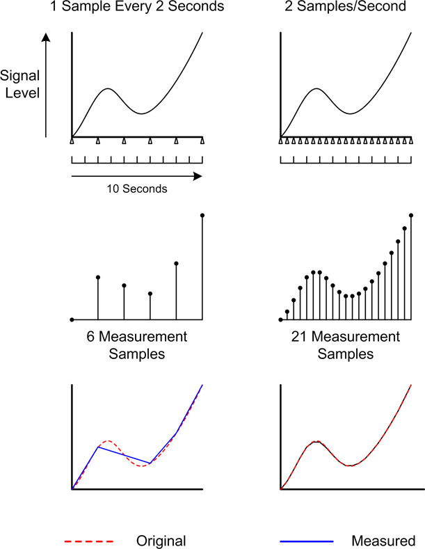
With analog inputs any changes in the analog signal between sample events are lost forever, and the result is only as faithful to the original as the number of samples per unit time permits. This is illustrated in Figure 2-30, which shows the difference between a signal sampled once every two seconds and the same signal sampled twice per second. Notice that the reconstructed result of the faster sampling rate is much closer to the original, but it is still not a 100% faithful reproduction.
Of course, not every application needs a high level of fidelity in order to accomplish the instrumentation objectives. In many cases it is perfectly acceptable to take data samples at intervals of several seconds, or even minutes. This is particularly true when the measured input doesn’t change very much within the sample period, such as might be the case with something like an oven, an air conditioning system, or a culture incubation chamber. Other applications, such as the conversion of audio to digital form, require very high sampling rates in order to accurately capture the highest frequencies of interest and maintain a high-fidelity representation of the original input.
Analog data is typically converted to digital form with a resolution, or data size, ranging from 8 to 24 bits per sample. Resolutions of less than 8 bits or greater than 24 are not readily available, but are possible. With an 8-bit resolution, the data will range in value from 0 to 255 (or from −128 to +127 if negative values are used). Again, one does not always need a high degree of precision for every application, and sometimes less is more than sufficient.
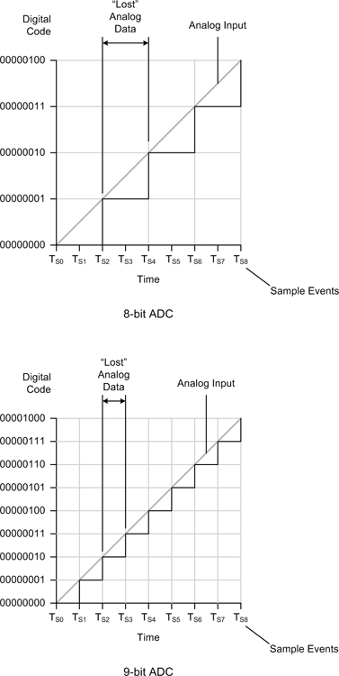
When converting from analog to digital (or vice versa), one will encounter an inherent limitation in the conversion referred to as quantization error. In general terms, this is the error between the original signal and the digital values, or codes, resulting from the conversion. As shown in Figure 2-31, the lower the resolution of the ADC, the more pronounced the quantization error becomes.
According to Figure 2-31 (which is only an approximation for purposes of discussion), a 9-bit ADC with a range of 512 possible values will generate a more accurate conversion than an 8-bit ADC with a range of only 256 possible values. The sampling events (the sample rate) are shown on the time axis as TS0, TS1, and so on. Note that it doesn’t matter if the 8-bit converter is sampled at a fast rate; it cannot do any better than its fundamental 8-bit resolution, although it will be able to detect and convert fast changes in the input that are within its resolution.
In Figure 2-30, the loss of fidelity at the slower sampling rate arose because of a lack of samples to accurately track the changes in the analog signal, not a lack of conversion resolution (the resolution isn’t even mentioned, actually). In Figure 2-31, it is the lack of resolution that results in the loss of fidelity due to quantization error.
The sampling rate and the sample resolution together determine how accurately an ADC can convert an analog signal to digital form. Sample resolution can be expressed in terms of volts/step, or, in other words, the measurable voltage difference between each discrete digital value in the converter’s resolution range. If we have an 8-bit converter with a maximum full-scale input range of 0 to 10 volts, each increment, or step, in the digital output code will be the equivalent of 0.039 volts. This can be expressed as:
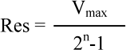
Therefore, a 10-bit converter with a Vmax of 10 V can resolve 0.00978 volts/step, a 12-bit device can resolve 0.0024 volts/step, and 16-bit ADC can resolve 0.0001526 volts/step.
This should be enough information about ADCs to get us started for now, so we will move on to the inverse of the ADC, the digital-to-analog converter. For more information about ADC devices and their behavior, refer to the references listed at the end of this chapter.
Generating analog data
The opposite of the ADC is the DAC, or digital-to-analog converter. These devices generate an output voltage that corresponds to a digital input value. Like ADCs, DACs have some inherent limitations in regards to resolution, and the devices also exhibit quantization.
Figure 2-32 shows the relationship between the resolution and the output update rate, or sample rate.
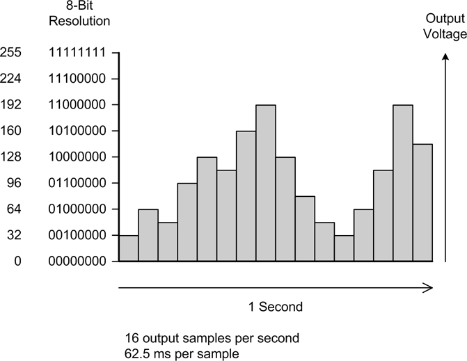
For many instrumentation and control applications the output sample rate is not a critical parameter, and something on the order of once or twice a second will suffice. This is assuming, of course, that whatever the DAC is intended to control does not need to change at a faster rate.
For some DAC devices, the output voltage range is established externally using a reference voltage. In other cases, the reference voltage is built into the DAC device itself. The output resolution is determined by the number of bits used to generate the output value, and is just the output voltage range divided by the number of possible digital input values. The actual accuracy of the output is a function of the linearity of the device.
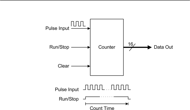
Counters and Timers
Counters and timers are essential components in many data acquisition and control implementations. Figure 2-33 shows a generic 16-bit counter with Run/Stop and Clear control inputs. When the Run/Stop input is high (true) the counter will increment an internal count value for each input pulse detected. Otherwise, it will ignore the pulse input. The Clear input allows the internal counter to be reset to zero. A counter does not need a continuous stream of input pulses; it can count random events as well. As implied in Figure 2-33, the length of time that the Run/Stop signal is in the Run state can be used to determine the rate (i.e., frequency) of the input pulses.
A timer is a device that also contains an internal counter, except that instead of counting external events it is counting either up or down until it reaches some specific value. Figure 2-34 shows a generic timer configured for single pulse output, and another version that has been configured for continuous pulse output by tying the output to the reset input.
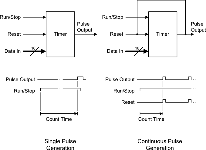
A 16-bit count value is loaded into the device via the data input lines. The Run/Stop input controls the counting action, and the Reset input restarts the counter either at zero (if it is counting up) or at the preloaded value (if it is counting down). Some timer devices also allow the current count value to be read out of the device.
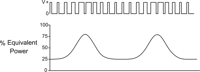
PWM
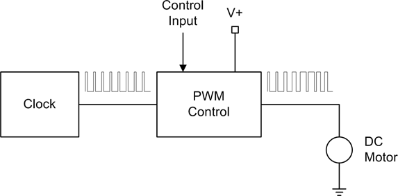
Pulse-width modulation (PWM) is a common form of output signal used to control lights, motors, and other devices. A PWM signal is a variable duty-cycle pulse, as shown in Figure 2-35. As the duty cycle increases, the average amount of power increases.
PWM is particularly effective for efficiently controlling DC motors. The RPM of a DC motor is proportional to the amount of power available to it. With PWM, unlike with an active linear control device such as a transistor, the average power can be modulated without wasting energy. A PWM signal can be generated directly from a digital source, with no DAC required. Figure 2-36 shows a block diagram of a PWM DC motor control.
Serial I/O
A serial interface is one wherein the data moves as a series of data bits over a single path, as shown in Figure 2-37. Serial data is typically implemented in one of two forms: synchronous or asynchronous. In a synchronous serial arrangement, there are one or two lines for transmitting data and a line (or two) for clock signals. The clock signals are used to inform the electronics at either end when a valid bit of data is present on the serial lines. An example of a synchronous serial interface is the low-level serial peripheral interface (SPI) feature found in some microcontroller and I/O ICs.

Notice in Figure 2-37 that device A is the source of the clock signal, so it effectively controls the data exchange rate, or speed, of the interface. Device B sends and receives data only when the clock is active, and only when it has been electrically selected via a special device select input (not shown here). The diagram shows a situation where data is valid on the falling edge of the clock signal. Also notice in Figure 2-37 that the falling edge of the clock occurs in the middle of the data bit position. Recall the “real-life” square wave from Figure 2-24: one can see that sampling (or, “latching,” as it is called) the data between the nastiness on the edges of the square waves in the data bit stream diminishes the risk of errors.
In an SPI interface, the clock is usually only active when the master device wishes to initiate communications with a peripheral device. Other types of synchronous interfaces may have the clock active all the time, and still others may utilize independent clock signals for both ends of the channel.
When connecting computing or instrumentation devices to one another, a more commonly encountered type of serial interface is the asynchronous serial interface. In this scheme there is no clock signal between the communicating devices, so the receiver electronics must synchronize on the data itself. To this end, the serial bit stream includes additional start, stop, and parity bits for each character of data. Figure 2-38 shows a greatly simplified diagram of an asynchronous communications channel using two Universal Asynchronous Receive-Transmitter (UART) devices. The RS-232 interface that was once a common feature on PCs is an asynchronous serial interface and was implemented in early versions of the PC using an Intel 8250 UART device. These types of devices can still be purchased, but it is also common to find the logical model of a more modern UART, such as the 16550, implemented within a custom gate array device as part of the chipset on a motherboard (now you know where the reference to “16550” in the serial port setup dialog box of your PC comes from, if you didn’t know before—it’s still there, it’s just not a separate part anymore). An interesting historical tidbit is the fact that in its original form the RS-232 specification set aside signals for timing—it could also be implemented as a synchronous interface. This is still defined in the specification but is seldom used nowadays in PCs.
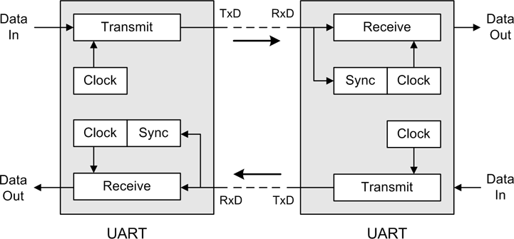
A modern UART chip contains all the circuitry necessary to implement one end of an asynchronous serial interface channel. In Figure 2-38, the box labeled “Sync” is responsible for detecting the incoming data stream and adjusting the receiver section’s clock to the data rate.
If an interface has signal lines for both sending and receiving data, it also has the capability for full-duplex operation. The term “full-duplex” means that an interface is capable of sending and receiving data at the same time. Interfaces that have only a single data path are typically half-duplex, meaning that the devices connected to the interface can only be a sender or a receiver at any given time, not both at the same time.
SPI and RS-232 are just two examples of serial interfaces. Some others are I2C, USB, RS-422, RS-485, MIL-STD-1553, FireWire, and Ethernet. They differ mainly in regard to how the interface operates electrically and the speed at which data can move across the channel. In Chapter 7 we will examine serial interfaces in more detail, and also explore some of the differences between full- and half-duplex operation.
Parallel I/O
Parallel I/O refers to a data communications channel where a set of discrete I/O lines is used to transfer a set of data bits in a single read or write operation. A common example of a parallel interface is the printer port on a PC, although in reality there is nothing unique about the printer port except that the pins have been preassigned to implement a printer interface. Figure 2-39 shows the pin-out and data transfer timing diagram for a PC printer port.
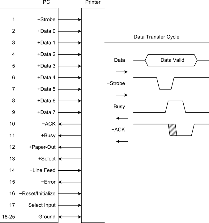
In Figure 2-39, the timing diagram (we’ll see more of these later) shows the general relationship between the Strobe, Busy, and ACK signals. The + and − symbols indicate the active-high and active-low true states of the signals, respectively. Also notice the shaded region in the ACK waveform. This indicates that the start of the ACK signal can vary, which is OK since the sender won’t attempt another transfer until ACK returns to the high state (False).
It is also possible to implement a parallel I/O channel using generic discrete I/O hardware, such as the plug-in cards available for the PC’s PCI bus. This is shown in Figure 2-40.
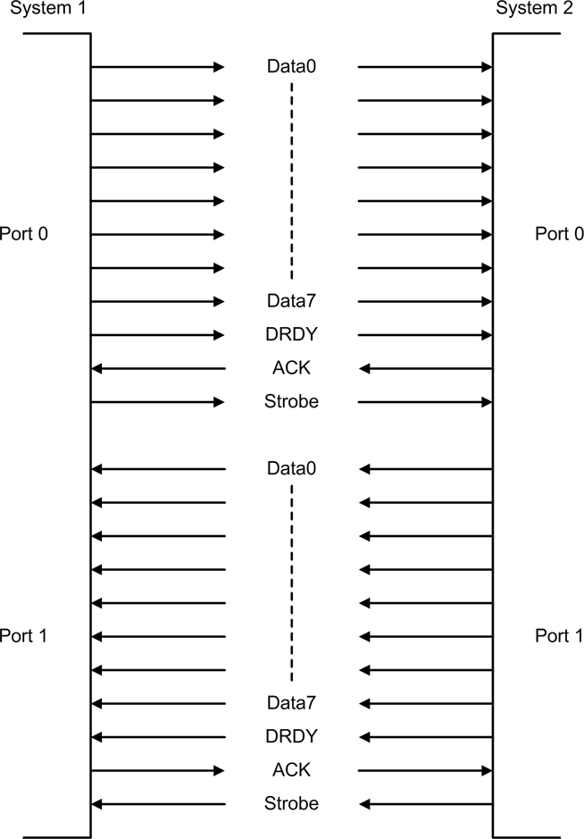
Notice that in both cases there are signal lines set aside for “handshaking.” These are the signals used to coordinate data exchanges between two devices, and are often implemented as “active-low” logic (meaning that the signal indicates True when it is low, rather than when it is high—this helps reduce false signals due to noise or other interference on the lines). In Figure 2-40, when one device has data available it will pull the DRDY (data ready) line low. The receiver will acknowledge this by pulling its ACK (acknowledge) line low and holding it low until the data transfer is complete. To initiate the transfer the sender pulls its Strobe line low, and the receiver uses this to latch the data into a buffer of some sort. When the receiver releases the ACK line, the sender is free to begin the whole process again for another set of data bits.
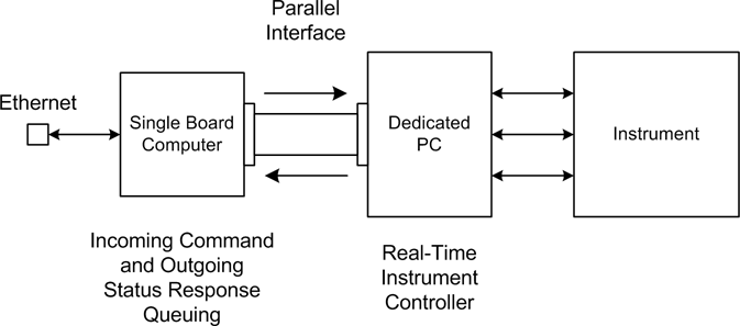
Parallel data interfaces have the intrinsic advantage of being able to move many bits of data at a time for every transfer cycle, and a parallel interface implemented entirely in hardware can move data at very high speeds. When implemented using software control for all of the functionality it won’t run as fast as it might otherwise, but it can still be a lot faster than an RS-232 interface. Figure 2-41 shows a block diagram for a system implemented in the late 1990s that used a single board computer (an industrial-type PC on a single PCB) to communicate with a dedicated controller PC that could not use a network interface for timing and resource reasons, but could support a dedicated bidirectional parallel interface.
Summary
In this chapter we’ve covered the basic concepts of charge, current, voltage, and resistance, and we’ve looked at some examples of how these concepts are applied. We also took a brief tour of interface electronics, but realistically, we’ve just barely scratched the surface. Nonetheless, you should now have enough basic background knowledge to feel comfortable with the data acquisition and control devices we will encounter as we go forward.
Suggested Reading
Electronics has become one of the cornerstones of modern civilization, and electronic devices of one type or another have now touched every corner of the globe. So it is no wonder that the field of electronics is vast and in a state of continuous change. Here are some books that I would recommend for those who would like to go deeper than what we could achieve in this chapter:
- The Art of Electronics, 2nd ed. Paul Horowitz and Winfield Hill, Cambridge University Press, 1989.
This book covers everything from the basics of electronic components through the design and construction of high-speed, low-noise laboratory-grade devices. It is written in a light and easy-to-read style, with just enough math to get the point across without becoming mired in details. The book contains numerous interesting examples of electronic circuits, and a good selection of “Bad Idea” circuits to avoid.
- Electronics, 2nd ed. Allan Hambley, Prentice Hall, 1999.
Suitable for use as a college text for an introductory class (or classes) in electronics theory, this book provides a formal and rigorous presentation, but the author does make a point of easing the reader into a subject, rather than dumping a pile of equations on the floor for the reader to sort out. It is a valuable resource for understanding the basics of the theory behind electronic devices and their applications.
- Data Conversion Handbook. Analog Devices Inc., Newnes, 2004.
Written by the engineering staff of Analog Devices, this book represents the definitive treatment of data conversion topics by the people who have designed some of the most advanced data conversion devices currently available. It includes coverage of topics such as the history of data conversion, sampled data systems, and data converter interfaces.