
Chapter 11. Instrumentation Data I/O
It is a capital mistake to theorize before one has data.
In Chapter 7 we looked at the various physical interfaces and signal protocols that you might encounter with instrumentation systems. Now we’ll look at how to use those interfaces to move data between the real world and our applications.
The data an instrumentation system collects or generates comes in a variety of formats and fulfills a wide range of needs. We’ll start this chapter with a discussion of interface formats and protocols, defining the basic concepts we will need for the upcoming software examples. Then we’ll take a quick tour of some packages that are available for interface support in Python: namely, the pySerial, pyParallel, and PyVISA packages.
Lastly, I’ll show you some techniques to read and write instrumentation data. We’ll take a look at blocking versus nonblocking I/O, asynchronous input and output events, and how to manage potential data I/O errors to help make your applications more robust.
Data I/O Interface Software
Over the years, computer interface hardware has evolved from simple devices using serial communications and I/O registers mapped into a computer’s memory address space to complex subsystems with their own built-in processors, onboard logic, advanced protocols, and complex API definitions. As the complexity grew, the number of unique interface methods and protocols also began to grow. As you might imagine, if a large system had to support more than just two or three unique interfaces, each with its own unique way of doing things, this could result in a significant hassle.
Early on, people began to realize that it didn’t make much sense for each device to have a custom interface, especially when many devices shared common internal functions and had similar capabilities. In order to rein in the impending chaos and establish consistent interfaces across different application domains, various industry standards organizations were formed. These organizations began to define guidelines and rules for interfaces and the software that would use them. These could then be applied to different types of equipment in a wide variety of situations. The Electronics Industries Association (EIA) published its initial definition of RS-232 in 1962, and after several revisions, it is still in use today. Various common standards have also been developed by other organizations, such as the American National Standards Institute (ANSI), the Institute of Electrical and Electronics Engineers (IEEE), and the Interchangeable Virtual Instrument (IVI) Foundation.
That being said, one must occasionally deal with exceptions. Although there are a number of common standards for communications and instrumentation interfaces, not every manufacturer follows them, and sometimes a device just doesn’t fit easily into an existing framework. If you want to use a device in your system that does things in its own special way, you’ll need to be able to accommodate that device. This is particularly true if you are planning to use an older instrument or device that might predate a more current standard.
Interface Formats and Protocols
Regardless of the type of connector used for a particular interface, or even the way in which data moves through an interface, the key thing is that data is moving between a host system (the master controller, if you will) and whatever devices or instruments are connected to it.
Naturally, when it comes to data acquisition and instrument control, there are multiple ways to get there from here. One approach is to use custom software with common interfaces to external instruments, such as serial and USB interfaces. Another way is to utilize industry-standard drivers and protocols that provide a consistent API across a range of physical interfaces, including serial, USB, GPIB, and bus-based hardware. Interface drivers that are based on the IVI standards are one example of this approach. In this section we’ll take a brief look at how various command and data protocols are implemented, at some of the more common standards and guidelines used to implement them, and at the physical interfaces commonly found in instrumentation devices.
The simplest way to interface a computer with the real world is through a serial or parallel port interface of some sort. The apparent simplicity is a result of the physical simplicity: the computer already (usually) has a serial or parallel interface of some sort, so the physical connection is typically just a cable. However, from a software viewpoint it may be anything but simple, especially with USB or GPIB. We’ll get to that in just a bit.
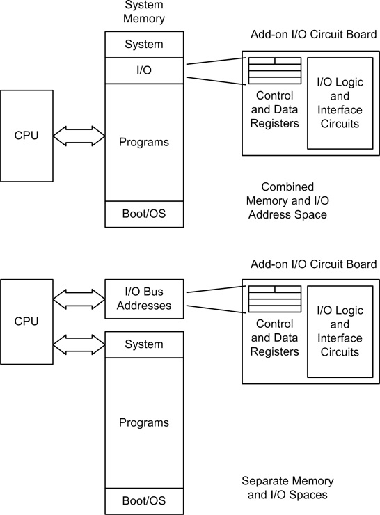
The other method, which we saw in Chapter 7, is the plug-in circuit board that is connected directly to the computer’s internal data and address buses. With an arrangement like this, the circuit board (or “circuit card,” as it’s often called) appears to the CPU (central processing unit) as just another address or set of addresses in memory space, I/O space, or both. Figure 11-1 shows how this works with a generic CPU that does not provide a separate I/O bus for peripherals (such as the Motorola 68000 family), and a CPU that incorporates a bus specifically for I/O functions (like the Intel processors found in most modern PCs).
The first generation of PCs used the Industry Standard Architecture (ISA) bus for add-on circuit boards. The earliest incarnations of the ISA bus, also known as the AT bus (it appeared in AT class PCs from IBM), took advantage of the Intel CPU’s built-in I/O bus and directly exposed the various add-on boards to the CPU in the form of registers. Later bus schemes, such as VESA Local Bus, EISA, and PCI, used special circuitry (called “chipsets”) to act as intermediaries between the CPU and the I/O devices. This resulted in more addressing flexibility, better support for direct memory access, and faster data rates. But regardless of the bus type, plug-in circuit boards still use registers to pass command and response data between the board’s circuitry and the CPU.
When working with I/O hardware that uses registers, a piece of software called a driver is employed to handle the low-level details of the interface. The driver provides an interface to programs that use the hardware, and it typically handles things like interrupts and bulk data transfers in a more or less transparent fashion. From the viewpoint of the application software, the driver appears as a set of function calls. From the viewpoint of the driver, the hardware appears as a set of registers in memory or I/O address space. Another characteristic of a driver is that it can be integrated into the operating system as an extension to its basic functionality. In modern operating systems, programs running at what is called the user level cannot usually access the underlying hardware directly, for various security and system-stability reasons. The operating system needs to be able to coordinate access to the hardware in the system to avoid conflicts and possible system failure.
Drivers might also be used to access a standard serial or parallel port, and they are always used with USB- or GPIB-type interfaces. In some cases, such as with a standard serial interface, the stock driver supplied with the operating system might be sufficient. In other cases, a special driver is needed to handle the interface. In those cases where software is provided to communicate with an external device using a common interface, I will refer to it as an I/O handler, rather than as a device driver. You can think of an I/O handler as something akin to a translator.
The upshot here is that whatever form the I/O takes, there is a driver or I/O handler of some type acting as an intermediary between the hardware and the application software. At the other end, in the hardware or external instrument, there are functions for handling the physical interface and communicating with the device’s hardware logic and control circuitry. Figure 11-2 shows the more common functional components one might encounter when interfacing with an external instrument or bus-based device connected to a host controller PC.
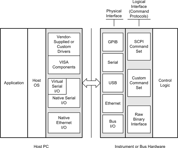
We will define the various acronyms in the figure and look at each component more closely in the following sections. For now, think of Figure 11-2 as a reference. I will refer back to it in later sections as we explore the various functional components within each level.
IVI—Interchangeable Virtual Instrument
In the instrumentation industry, the IVI suite of standards is becoming commonplace for Windows platforms, and many instrument manufacturers now provide IVI-compliant drivers. Aimed mainly at instrumentation applications, the IVI defines a standard set of instrument interfaces and commands. Prior to the creation of the IVI suite of standards, there were multiple standards in use, with the most notable being the Standard Commands for Programmable Instruments (SCPI, sometimes pronounced “skippy”) and the newer Virtual Instrument Software Architecture (VISA) standards. Each vendor could, and sometimes did, do things a little differently in its own special way.
The SCPI standard defines a standard set of commands for instrumentation, and VISA defines a common API usable with different I/O interfaces, such as GPIB and VXI. SCPI and VISA are now both part of the IVI suite. The primary focus of these standards is to define common interfaces that help to reduce, or eliminate, the necessity of treating each instrument as a unique programmable object. Note that while SCPI and VISA are now part of the overall IVI suite, they are actually two different things.
If you will be using instruments such as DMMs and counters in your instrumentation setup with GPIB interfaces, the odds are good that you will need to know about SCPI. If you want to take advantage of a manufacturer’s VISA drivers, you’ll need to know about those as well. In just a bit we’ll take a look at how to use VISA drivers with Python for both Windows and Linux systems.
There are, of course, situations where things like SCPI or VISA simply aren’t available. In these cases there may be no choice but to either try to use whatever interface software the manufacturer did provide or, lacking that, just write your own. That said, I should point out that writing a device driver or I/O handler is often a nontrivial task, and you really should avoid it if at all possible.
IVI-compliant drivers
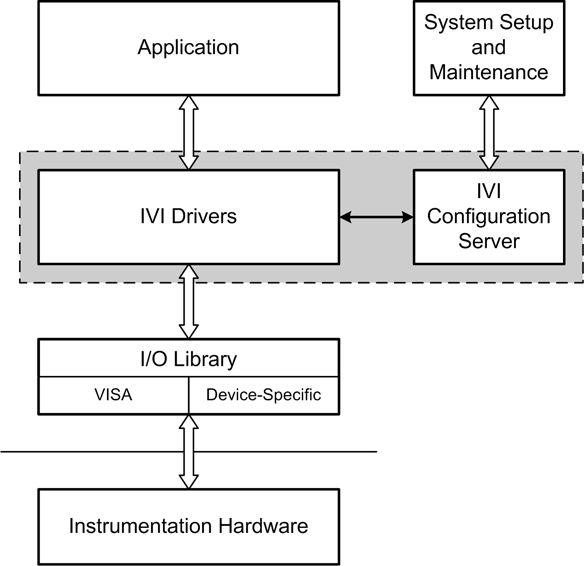
Depending on the complexity of the project and the operating system on the host PC, it may make more sense to adopt something like the IVI drivers instead of attempting to “roll your own” API. The IVI Foundation standards define the driver architecture for various classes of instruments and interface hardware. The IVI approach is based on the notion of shared software components with common functionality, so that the API for one instrument looks much like the API for another. It is based on the VISA I/O standard (which we will encounter shortly), and also incorporates the SCPI protocol standard. Figure 11-3 shows an overview of the IVI architecture.
IVI-compliant software can offer some significant advantages. These include state caching, multithreaded drivers, simulation capabilities, and instrument interchangeability. One of the claims made for IVI is that its standardized interface handles the details between different instrument types, thus allowing the system implementer to focus on the data handling and display software, rather than having to deal with unique interface code for each instrument in the system. For the most part this is true, but only insofar as it applies to commercial off-the-shelf (COTS) software that is IVI-compliant. If you need to access an instrument using a programming language that isn’t supported (such as Python), or use data capture and analysis tools that don’t come with IVI interface capabilities already built in, you will need to do some work to get things to play nice with one another.
One potential downside to IVI is that fully IVI-compliant (and IVI-certified) drivers are available only for the Microsoft Windows platform. This is stated clearly in the IVI specifications published by the IVI Foundation. Although some instrumentation vendors have created “IVI-style” drivers for their products that will work with Linux systems, if you’re looking for true cross-platform compatibility across a variety of vendors you may want to take this into consideration.
VISA—Virtual Instrument Software Architecture
VISA is a widely used interface I/O API specification for communicating with instruments connected to a PC using GPIB, VXIbus, serial, Ethernet, or USB-type interfaces. The VISA standard is also a core component in the IVI suite.
The VISA library defines a standardized API using a Windows DLL module, typically named visa32.dll. VISA also supports the Microsoft Component Object Model (COM) technology. If applications are written against the VISA standard, they should be generally interchangeable with VISA driver implementations from different vendors.
Not all instruments come with VISA drivers, and for some VISA support may be an optional add-on at the time of purchase. GPIB-interface products, such as the plug-in cards sold by National Instruments (NI), usually do come with VISA drivers, and a Linux version is readily available as well. Agilent also sells GPIB interfaces with VISA components, and Agilent recommends a VISA interface for Linux that is available from a third-party source.
SCPI—Standard Commands for Programmable Instruments
The SCPI standard defines the syntax, command structure, and data formats for use with programmable instruments. SCPI does not define the actual physical interfaces (GPIB, RS-232, USB, etc.), meaning that it is an interface-neutral standard. SCPI was preceded by the IEEE-488.2 standard, which is similar but with a more limited scope.
SCPI commands are ASCII strings. Responses may also be ASCII strings, although in some cases they are binary data (for example, when transferring bulk measurement data). SCPI commands are organized into instrument classes, each of which defines a baseline set of commands. Instruments that support the SCPI protocol do not require the low-level VISA I/O functions so long as there is some way available for the host system to communicate with the instruments (remember that SCPI is a command protocol, so it is interface-neutral). Figure 11-4 shows the instrument model employed by the SCPI standard. The SCPI functionality resides in the logical interface layer in the instrument interface, as shown previously in Figure 11-2.
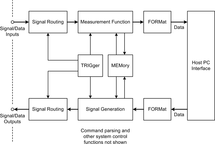
Not all of the functions shown in Figure 11-4 are used in all instruments. Some instrument types, such as temperature sensors or digital multimeters, may be input-only devices. For these, there would be no signal generation section. Others, such as some types of spectrum analyzers, might incorporate both input and output functions, so they could include all of the SCPI model (or at least a good portion of it).
The commands available for a given instrument are based on the instrument type, or class. The SCPI 1999 standard defines eight instrument classes, each of which utilizes a particular subset of the SCPI commands:
Chassis Dynamometers
Digital Meters
Digitizers
Emissions Benches
Emission Test Cell
Power Supplies
RF & Microwave Sources
Signal Switchers
Some of the terminology in these class names might not be intuitively obvious. In SCPI parlance, a digitizer is a device designed to measure voltage waveforms over time—in other words, an oscilloscope or a logic analyzer. A signal switcher is an instrument designed to control the path of signals through some kind of routing or switching network. This might be as simple as an on-off switch, or as complex as a multipath input-output switch matrix. Several instrument manufacturers produce devices that incorporate signal-switching capabilities along with optional data acquisition or control functions. The Agilent 34970A Data Acquisition Switch Unit and the Keithley 3706 System Switch/Multimeter are examples of these types of devices.
SCPI commands are organized as related groups of instructions. A
group is composed of a primary, or root, command,
and each root command has a number of optional parameters. One example
of a command group is the MEASure command. (SCPI allows commands to be
abbreviated, as indicated by the use of capitalization; so, for
example, instead of using MEASure
one could use MEAS.)
Figure 11-5 shows a
simplified command tree diagram for the MEASure command as it might be used with a
digital multimeter. To build up a command string, you would start at
the left side with MEASure and then
move to the right through the tree, picking up the necessary parameter
keywords as you go.
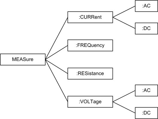
Here is an example of a SCPI command for use with a digital multimeter, such as an Agilent 34405A DMM (refer to Figure 6-4) with a GPIB interface:
MEASure:VOLTage:DC?
Assuming that access to the GPIB port or interface device has already been established, and the instrument has been correctly initialized, this command instructs the instrument to take a DC measurement using whatever autoranging is appropriate and return the result (as implied by the question mark at the end of the command string).
Here is an alternate command sequence for the Agilent 34405A DMM to set the DC input range and then acquire a measurement:
CONFigure:VOLTage:DC 1, 0.0001
TRIGger:SOURce IMMediate
INITiate
FETCh?
This command sequence configures the DC input for the 1 V input
range with a 0.1 mV resolution and sets the measurement trigger mode
to immediate. The INITiate command places the instrument in the
“wait for trigger” mode, which in this case is immediate, so the
instrument begins taking continuous readings. The FETCh command returns the most recent voltage
reading.
As mentioned earlier, the SCPI commands can be abbreviated. Here’s what the preceding command sequences look like in short form:
MEAS:VOLT:DC?
and:
CONF:VOLT:DC 1, 0.0001
TRIG:SOUR IMM
INIT
FETC?
A description of the entire SCPI specification would be beyond the scope of this book. For more information, consult the section Suggested Reading. You should also refer to the programming documentation supplied with each instrument you intend to use to determine exactly how it implements SCPI. While many instrument manufacturers follow the SCPI standard, there may be variations to accommodate special features.
Unique protocols
Some instruments (e.g., some low-cost DMMs) use command and
data protocols that are unique to that particular model. For example,
the tpi 183 has a 3.5 mm jack built into the side of the
meter and continuously outputs a stream of RS-232 data at 1,200 baud.
The type of data is determined by the meter’s manual control settings
(a large rotary switch)—there is no way to set it via the serial
interface. The output is a string of ASCII characters, and the format
is defined as FAR DDDDDDT. The
character in the F position is the
function code (0 to B), A is
the manual or autorange mode (0 or
1, respectively), and R is the range code (0 to 5).
This is followed by a space character (which is somewhat unusual) and
six ASCII characters for data in floating-point format (the DDDDDD part of the format string). The
T character indicates the end of
the output string.
Although this interface may be unique to the tpi 183, it is by no means a singular example. Many instruments—especially older units—have unique interface protocols. Even some modern USB-type devices have their own unique command and data interface protocols.
Another example is the command and response protocol used with devices connected to an RS-485 bus. A common scenario is where one device is designated as the master (typically the host PC), and the other devices respond only when they receive commands addressed specifically to them. In this case, a device identifier must be included with each command on the RS-485 bus, alerting the relevant device that this command is intended for it. The other devices will “hear” the command, but they will not respond to it. One possible format for the command and response messages s shown in Figure 11-6.

Notice in Figure 11-6 that
the response always begins with /0,
because in a scheme like this the master controller is typically
assigned a device ID of zero. Since there is only one ASCII digit
available for the device ID number, this protocol will only be able to
support 15 unique devices, addressed as 1 through F. From Figure 11-6 we can also infer that there
are 256 possible command or response codes (assuming that hexadecimal
notation is used, i.e., 00 through
FF). The number of characters sent
as command or parameter data or returned as response data is variable
and is defined by the command type. A command message is terminated
with a ! character, and a response
is terminated with a # character.
Remember that this is just one possible protocol, although it is
actually modeled on real products that are commercially available. How
the command and response messages are defined is ultimately up to the
engineers designing the product.
Python Interface Support Packages
There are several I/O support packages available for Python to help with the implementation of various types of interfaces in Python applications. These include serial, parallel port I/O, USB, and VISA-type instrumentation interfaces, including GPIB. In this section we will take a quick look at three different packages, all of which aim for easy portability between platforms (Windows and Linux, primarily).
pySerial
The pySerial package, written and maintained by Chris Liechti, encapsulates the functionality necessary to communicate with a serial port from a Python program. It is available from http://pyserial.sourceforge.net. pySerial will automatically select the appropriate backend (the physical interface and its OS-supplied driver), depending on the host OS, and it supports the Windows, Linux, BSD, Jython, and IronPython environments.
A single class, Serial,
provides the necessary functionality with the same set of methods for
all platforms, and once installed it is straightforward to use.
Assuming that there is something connected to the serial port that can
display the data written from Python, sending a string is as simple as
this:
>>>import serial>>>sport = serial.Serial(0)# open a serial port >>>print sport.portstr# print port string >>>sport.write("Port opened ")# write a string with CR and LF
When these lines are executed from the Python prompt, it will respond with:
COM1
(assuming that COM1 was used, of course), and at the other end of the connection you should see:
Port Opened
When we’re done with the serial port we can close it gracefully (it can be reopened later on, if need be):
>>> sport.close() # close portpySerial also supports various port
configuration parameters and timeout values, and it provides methods
such as read(), write(), and readln().
If there is no serial port available, which is typical with notebook and netbook computers, you’ll see an error traceback that looks something like this:
Traceback (most recent call last):
  File "<stdin>", line 1, in <module>
  File "c:APython26libsite-packagesserialserialwin32.py", line 30,
    in __init__
    SerialBase.__init__(self, *args, **kwargs)
  File "c:APython26libsite-packagesserialserialutil.py", line 201,
    in __init__
    self.open()
s  File "c:APython26libsite-packagesserialserialwin32.py", line 56,
    in open
    raise SerialException("could not open port %s: %s" % (self.portstr,
    ctypes.WinError()))
serial.serialutil.SerialException: could not open port COM1: [Error 2]
The system cannot find the file specified.
You can also create a serial port instance without actually
opening the port by simply not passing any parameters to the Serial object’s initialization
method:
>>>import serial>>>sport = serial.Serial()>>>sport.baudrate = 19200>>>sport.port = 0
Now that the serial port object has been instantiated and some
basic parameters defined, it can be opened and closed as necessary.
The isOpen() method is used to
check the state of the serial port:
>>>sport.open()>>>sport.isOpen()True >>>sport.close()>>>sport.isOpen()False
Tables 11-1 through 11-6 provide a summary of some of the methods available with pySerial, organized by functional category. In all likelihood you won’t need more than a handful of these, but pySerial does provide a fairly comprehensive suite of methods for dealing with serial communications. Even some of the more arcane capabilities of RS-232 are supported.
Method | Description |
| Opens (or reopens) the port using the current settings. |
| Closes the port but does not destroy the port object. It may be reopened later. |
| Returns |
Method | Description |
| Reads |
| Reads a string of
characters until an end-of-line ( |
| Reads a list of lines
until the read timeout occurs. The |
| Outputs the given string over the serial port. |
| Writes a list of strings to the serial port. |
Method | Description |
| Clears the input buffer, discarding all data currently in the buffer. |
| Clears the output buffer, aborting the current output and discarding all remaining data currently in the buffer. |
| Returns the number of characters currently in the input buffer. |
| Returns the number of characters waiting in the output buffer. |
Method | Description |
| Returns the current baud rate setting. |
| Sets the port’s baud rate. This method cannot be used if the port is already open. |
| Returns the current byte size setting. |
| Sets the data character bit size. |
| Returns the current DSR/DTR flow control setting. |
| Sets the DSR/DTR flow control behavior. |
| Returns the current parity setting. |
| Sets the port parity. |
| Returns the current port setting. |
| Sets the port number or name. |
| Returns the current RTS/CTS flow control setting. |
| Sets the RTS/CTS flow control behavior. |
| Returns the current stop bits setting. |
| Sets the number of stop bits to use. |
| Returns the current timeout setting. |
| Sets the read timeout period. |
| Returns the current write timeout setting. |
| Sets the write timeout period. |
| Returns the current XON/XOFF setting. |
| Sets the XON/XOFF flow control behavior. |
Method | Description |
| Returns a list of baud rates supported by the serial port. |
| Returns a list of the character bit sizes supported by the serial port. |
| Returns a list of parity bit settings supported by the serial port. |
| Returns a list of stop bit settings supported by the serial port. |
Method | Description |
| Returns the state of the Carrier Detect line. |
| Returns the state of the Clear To Send line. |
| Returns the state of the Data Set Ready line. |
| Returns the state of the Ring Indicator line. |
| Sets the Data Terminal Ready line to the specified state. |
| Sets the Request To Send line to the specified state. |
pySerial does not support RS-485 interfaces directly, but it works fine with RS-232–to–RS-485 converters that provide half-duplex auto-turnaround capability. It will also work with USB‒to–RS-485 converters, provided that they use a virtual serial port (for Windows) or a tty-type device entry in the /dev directory (for Linux). An experimental implementation of an RFC 2217 server is also provided with the pySerial package.
For installation and additional usage instructions, refer to the pySerial website.
pyParallel
pyParallel (http://pyserial.sourceforge.net/pyparallel.html) is a companion project to pySerial by the same author. The purpose of pyParallel is to encapsulate access to a parallel port by a Python program in a platform-independent manner (refer back to the discussion of parallel ports in Chapter 2 if you need a refresher). At present, it supports only Windows and Linux.
Unlike pySerial, pyParallel has no open or close methods. If instantiated with no port parameter, pyParallel will attempt to use the first available parallel port. Optionally, you can specify a particular port name as a string.
Here’s a simple example of how it can be used:
>>>import parallel>>>pport = parallel.Parallel()# open first available parallel port >>>pport.setData(0x55)>>>pport.setData(0xAA)
This will write the value 0x55 to the parallel port, followed
immediately by the value 0xAA.
Table 11-7 lists the methods
available.
Method | Description |
| Applies a byte value to the data pins of the parallel port |
| Sets the Data Strobe
line to |
| Sets the Auto Feed line
to |
| Sets the Initialize
line to |
| Reads the state of the Select line |
| Reads the state of the Paper Out line |
| Reads the state of the Acknowledge line |
Notice that pyParallel does not provide functions to read the Busy or Error inputs. However, pyParallel does allow you to directly manipulate the handshaking output lines on the port.
On Windows machines, pyParallel requires direct access to the physical port hardware. It cannot be used with USB parallel port adapters, so it won’t work on a notebook or netbook with only USB ports. It also does not support Extended Parallel Port (EPP) functionality.
Sending data to an external device via pyParallel involves outputting byte values one at a time under software control. This may sound clumsy, but there really is no other way to do it, short of using smart hardware with built-in flow control management and internal buffering capabilities. When communicating with a printer the program must, at a minimum, set and clear the Data Strobe and check the Acknowledge line coming back from the printer.
The parallel port on a PC isn’t restricted to just sending data to a printer, however. An interesting example of how you can drive an LCD display from a parallel port can be found at http://pyserial.svn.sourceforge.net/viewvc/pyserial/trunk/pyparallel/examples/.
Other interesting uses for a parallel port include controlling a DAC device, sensing discrete digital inputs, and using the 8 bits of output to control relays or other devices. The downside is that the port circuitry isn’t designed to handle very much current, so external interface circuitry is often required.
PyVISA
The PyVISA package provides a Python API for an IVI-standard VISA driver on Windows, or an IVI-compatible VISA driver for Linux systems. It uses a driver DLL or library file provided by an instrument vendor. On Windows machines, the package expects to find a DLL by the name of visa32.dll in the path, typically in C:WINNTsystem32. For Linux systems, National Instruments (NI) supplies an IVI-compliant VISA driver as a shared object library module (the Linux equivalent of a DLL on Windows systems), called libvisa.so.7. This file usually resides in /usr/local/vxipnp/linux/bin.
The NI Linux version of visa32 specifically supports the following distributions:
Red Hat Enterprise Linux Workstation 4
Red Hat Enterprise Linux Desktop + Workstation 5
SUSE Linux 10.1
openSUSE 10.2
Mandriva Linux 2006
Mandriva Linux 2007
Refer to the section Suggested Reading for more information about the NI VISA driver.
For Windows, you shouldn’t have to do a lot of digging to find what you need. Modern instruments with IVI-compliant interface capabilities typically come with a VISA driver for the Windows platform, so if you don’t have the original CD that came with an instrument you may want to look around and see if you can locate it, or perhaps one from a similar instrument. You may also be able to download the VISA components from an instrument vendor’s website.
VISA, and by extension PyVISA, supports serial, GPIB, GPIB-VXI, VXI, TCP/IP, and USB interfaces. We will be using VISA primarily to interface with GPIB-capable devices. A simple example of PyVISA in action looks like this:
>>>import visa>>>dmm = visa.instrument("GPIB::2")>>>print dmm.ask("*IDN?")
This tells the VISA driver that we want to use the instrument
with GPIB address 2 as the object dmm. The dmm.ask method sends the string specified
("*IDN?", in this case). It then
returns the instrument’s response, which should be the device’s
internal identification string.
You can find more information about PyVISA at the project’s home page, located at http://pyvisa.sourceforge.net.
VISA provides far too many different functions to go into all of them here. For a detailed look at VISA itself, the VPP-4.3 VISA library reference is available from the IVI Foundation.
Alternatives for Windows
There is an OSS project called PyUniversalLibrary that is developing a wrapper for Measurement Computing’s Universal Library API. According to the website it is not 100% complete, but it does have enough functionality to be useful. You can find out more about it here: https://code.astraw.com/projects/PyUniversalLibrary.
The UNC Python Tools package contains, among other things, a wrapper for National Instruments’s older NI-DAQ drivers. It is available from http://sourceforge.net/projects/uncpythontools/.
Using Bus-Based Hardware I/O Devices with Linux
Plugging an interface into a Windows machine is usually straightforward, and vendors typically supply interface drivers with their products. With Linux, an instrumentation device that uses a serial, GPIB, or USB port to communicate isn’t really a problem in most cases. However, when it comes to the cards that plug into the PC’s internal PCI bus, things get more complicated. In Chapter 5 we looked at what goes into an extension to allow it to serve as a wrapper for a DLL used with Windows to access a device connected to the internal bus of a PC. In the realm of Linux, each I/O device requires a driver written specifically for the Linux environment, along with whatever tools and utilities the device might need to configure its internal settings. Many instrumentation manufacturers simply don’t support Linux, at least not directly. This usually isn’t an intentional snub; there just aren’t enough Linux systems being used in instrumentation applications (yet) to justify the effort and expense of supporting two different versions of the interface software. There is, however, a project called Comedi that aims to provide a way to connect instrumentation interface hardware to PCs running Linux.
The Comedi project
The Comedi project was started in 1996 by David Schleef as a collection of low-level drivers to allow a Linux system to communicate with various types of data acquisition and digital interface cards. It is an open source project and is currently hosted at its own website, http://www.comedi.org.
The comedi package is a combination of three complementary software components. The first component is a generic, device-independent API. This interacts with a collection of Linux kernel modules that provide the interface support for the generic API (the second component), and lastly there is a library of functions that provides an interface to configure various cards (the third component). The Comedi team works with hardware vendors (whenever possible) to gather information, obtain hardware for test and verification, and develop the drivers. In one sense, you might say that Comedi is the Linux corollary to the IVI suite of drivers.
If you want to download and build Comedi yourself, make sure you get both the comedi and comedilib packages. You might also want to get the comedi_examples file.
Comedi hardware support
Comedi supports the following interface hardware manufacturers, to one degree or another:
ADLink
Advantech
Amplicon
Analog Devices
ComputerBoards
Contec
Data Translation
Fastwel
General Standards Corporation
ICP
Inova
Intelligent Instrumentation
IOTech
ITL
JR3
Keithley Metrabyte
Kolter Electronic
Measurement Computing
Mechatronic Systems, Inc.
Meilhaus
Micro/sys
Motorola
National Instruments
Quanser Consulting
Quatech
Real Time Devices
Sensoray
SSV Embedded Systems
Winsystems
Not every card from every vendor is supported, but with over 400 different types (and growing), Comedi covers a lot of territory. For a complete list, see the Comedi website.
Using comedi with Python
comedi is shipped with the ability to use the Simplified Wrapper and Interface Generator (SWIG) to generate a wrapper for comedilib. You can learn more about SWIG at http://www.swig.org. There is also a discussion group on Google that is a good first place to look if you encounter problems with comedi.
Data I/O: Acquiring and Writing Data
Now that we have some idea of what to expect in terms of the software we’ll need to interact with instrument hardware, let’s take a look under the hood and see how we can put it to work for us.
Basic Data I/O
When considering data acquisition, there are basically two types of data sources: external instruments, and data acquisition hardware installed in the computer itself. In both cases there is a transaction that occurs between your application software and the device. Sometimes the transaction is direct, such as when accessing the hardware registers of a device directly from the application-level code. This style of interface programming is rather rare nowadays, as the underlying operating system tends to prohibit direct hardware access by user-level code. In most cases, it will involve an intermediary such as a driver with a vendor-defined API (recall Chapter 5), or an interface library (e.g., pySerial).
When acquiring data from an external device, or sending data (e.g., a command) to a device, there are several ways to get there from here. If you want to send data, the first, and most obvious, approach is to just write the data to the port or device and let it go at that. When you want to read data, the obvious approach is to simply read the data on demand.
Both of these methods assume that when the device is sent a command or queried for data it will automatically and immediately perform whatever hardware functions are necessary to convert the data into an internal register address, an internal command code, or a return value. For the most part, this is a valid assumption. But there can be situations where things don’t work out like you might expect. Instead of a successful write operation, an error might occur, or the device’s driver API function might take a while to return or, worse still, not return at all.
Reading data
When reading data from a bus-based device, the device’s interface will typically return a binary value that can be used immediately. There is no need to send a command, per se; you can just use a function call. With an external instrument, on the other hand, the commands and data are typically in the form of ASCII strings and utilize a command-response format. ASCII-to-binary conversions can be handled fairly easily in Python.
Instruments that utilize SCPI will typically return strings
containing a numeric value, or multiple numeric values separated by
commas. Fortunately, Python can easily deal with numeric data in a
string format. Assume that we have an instrument that returns
something like "+4.85510000E-01"
when queried for a measurement. In the following code snippet, the
hypothetical function getDataResponse() will return a string
containing the instrument response string, or it will return None. We can use Python’s float type object
constructor to do the necessary conversion for us:
raw_data = getDataResponse(instID)
if raw_data:
    data_val = float(raw_data)
If raw_data is not None, the variable data_val will contain 0.48851, as expected.
Let’s look at another example, this time involving more than one
return value in response to a measurement command. Assume that an
instrument returns four values when queried, as the string "+5.50500000E00, −2.66000000E-01, +8.24000000E01,
−6.34370000E00". In Python, it is very easy to convert a
string of comma-separated values into a list of strings. The following
code snippet can be used to deal with a situation like this:
data_val = []
data_str = getDataSet(instID)
raw_vals = data_str.split(",")
for raw_data in raw_vals:
    data_val.append(float(raw_data))
After this, the list variable data_val will contain four floating-point
values:
[5.5049999999999999, −0.26600000000000001, 82.400000000000006,
 −6.3437000000000001]
The numbers look a bit odd due to the way that Python handles the string–to–floating-point value conversions, but they are essentially the same numbers as in the original string. The oddness is a result of the way that floating-point values are handled in the CPU (Python doesn’t make it pretty unless you ask it to do so).
If you are acquiring data from an instrument that returns an ASCII string that contains something other than just numeric data, you may need to do some type of parsing to extract the specific sections of interest from the returned string. The ASCII data will also need to be converted into a binary format of some type. The RS-485 interface we looked at earlier is an example of this type of situation.
In some cases the return string may contain a mix of numeric and nonnumeric characters, and not always in a fixed format. The tpi 183 DMM we looked at earlier generates a fixed-format data string. This is very easy to deal with, as all you need to do is extract a slice from the string that contains the data (see Chapter 3 for more on slices in Python). However, this is not always the case; sometimes the length of the data portion, and even the leading header characters, of the return string can vary.
If you’re dealing with an instrument or device that employs a format with a fixed starting position for the data and uses an end marker character, you can obtain the position of the end marker in the string and use a slice to pull out what you need. If the starting position is not fixed, you’ll need to scan through the string and find the start of the data field before you can use a slice to extract it.
Writing data
As mentioned earlier, accessing a bus-based device typically involves just calling a function in the device’s API. There are no commands, as such, but it is common to write parameter values to the device, or call a function to start or stop some action (such as, say, a timer or clock function).
Writing ASCII data (i.e., commands and parameter values) to an external instrument that utilizes SCPI, or a unique command format, involves creating the necessary command string, writing it, and then waiting for the instrument to respond. In this command-response scenario the instrument returns data only when requested to do so; it does not spontaneously send data on its own. Also, in some cases there is no response.
For example, let’s assume that we have a GPIB instrument such as a programmable power supply. This example is based on the Agilent E364xA series, which includes some non-SCPI commands that I won’t cover here. For now, I’ll just use the following commands:
OUTPut
    [:STATE] {ON|OFF}
    [:STATE]?

[SOURce:]
    CURRent
    CURRent?
    VOLTage
    VOLTage?

MEASure
    :CURRent?
    [:VOLTage]?
The curly braces around the ON|OFF parameters indicate a choice. Also,
notice that some of the items are in square brackets, including the
key command SOURce. This indicates
that these are optional, and whatever parameter is in square brackets
is the default. So, in the case of the MEASure command, if the command is given
as:
MEAS?
it will return the voltage at the outputs of the power supply. To get the current, the command must explicitly specify it:
MEAS:CURR?
Since the SOURce command is
optional, the following set of command strings will set the output to
5.1 volts DC and the current limit to 1.0 amperes:
VOLT 5.1
CURR 1.0
If we wish, we can also control the output from the supply using
the OUTPut command, like so:
OUTP:OFF
SOUR:VOLT 5.1
SOUR:CURR 1.0
OUTP:ON
This disables the output before changing the V and I
parameters.
To read back the settings, we can use the SOURce:VOLTage or SOURce:CURRent commands with a question mark
to indicate a query:
VOLT?
This will return a response like this:
5.00000
To see what is really happening on the output terminals we can
use the MEASure command, like
so:
MEAS:CURR?
This returns (for example):
0.20000
This command will read the output voltage:
MEAS?
and it returns:
5.00000
Finally, we can check to see whether the supply’s output is
enabled or not using the query form of the OUTPut command:
OUTP?
If the supply is enabled, it will return an ASCII “1”; otherwise, a “0” is returned.
I haven’t indicated how the commands are sent and the response
returned because there are several ways to do this, such as serial,
USB, and GPIB. But let’s assume that there is a function called
sendCommand() that will take care
of this for us. For this example we’ll create a function called
setPowerSupply() that will accept
the voltage and current parameters and send them to the
instrument:
def setPowerSupply(volts, current):
    rc = OK
    volts_str = "%2.2f" % float(volts)
    current_str = "2.2f" % float(current)

    cmd_str = "VOLT " + volts_str
    rc = sendCommand(instID, cmd_str)
    if rc == OK:
        cmd_str = "CURR ", current_str
        rc = sendCommand(instID, cmd_str)

    return rc
This seems rather straightforward, but there are some things going on that might not be readily obvious.
After rc (the return code) is
preset to OK (to be optimistic),
the input parameters volts and
current are converted to string
representations. Notice that the format is specified as %2.2f. This will create a string
representation that the instrument can easily handle. Also notice that
the input parameters are used to create float variable objects, which
are then inserted into the string variables. If the input parameters
are given as floats, nothing changes, but if the input parameters are
integers they will be converted. Also, this function will accept
string representations of integer or floating-point values for either
parameter.
This, by the way, is a very handy and powerful trick. It will
deal with almost any numeric value, in any valid format, that you
might care to throw at it, and gracefully convert it to a
floating-point type. It will fail if an input parameter is a
nonnumeric string, a hex value in string format, an
n-tuple, or a dictionary, but these cases can
easily be trapped and handled using a try-except construct.
Next, the sendCommand()
function is called. This might use GPIB, or it might be the access
function for serial I/O. It really doesn’t matter how the command is
sent, as long as the instrument gets it.
So now that we’ve seen how to send a command, how can we tell if the instrument actually accepted the command and did what the command specified? In the case of a power supply, we would mainly be interested in knowing if the output is active and what the output values actually are. Sensing the output state (On or Off) is straightforward, as we’ve already seen, but determining if the output levels are at, or near, the commanded values can be somewhat challenging.
The reason is that we’ve now made the leap from digital to analog, and the analog world is full of subtle variations. Depending on the accuracy of the instrument, if we command it to generate a 5.000 V DC output, in reality the voltage on the output terminals might be 4.999 V DC, or anything within the tolerance range of the device. The following snippet shows one way to implement a return value check with upper and lower tolerance bounds:
def testDelta(testval, targval, tolerance=0.001):
    testval_float = float(testval)
    targmax = float(targval) * (1 + tolerance)
    targmin = float(targval) * (1 − tolerance)
    if (testval_float >= targmax) or (testval_float <= targmin):
        return False
    else:
        return True
The float object conversion is also used here, as in the previous example. This ensures that all the internal variables will be float types.
If the value passed to testDelta() is within some +/− range of the
target value (targval), the
function will return True;
otherwise, False is returned. The
tolerance check is symmetrical around the target value, as shown
in Figure 11-7.
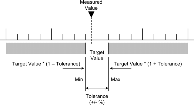
If we wanted an asymmetrical tolerance check, we would need to specify an offset relative to the target value. Between the tolerance range and the offset, we could move the acceptance window to any position and width necessary.
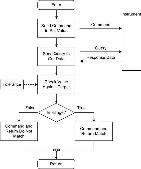
Figure 11-8 shows a flowchart for a function used to set the output of an instrument (such as a power supply or some other type of analog output), and then read the output and compare the value returned to the original commanded value. Depending on the system, just checking the actual output value and then reporting an error (if any) might be sufficient, but as we’ll see in a just a bit we could also attempt to retry the command, or initiate a system shutdown.
Now, at this point you may be wondering: “Why would I want to go to all that trouble?” Good question, and here’s an example of why you might want to do that.
With a programmable power supply you can set the maximum current as well as the output voltage. What happens when the current exceeds the programmed limit? Some power supplies can be configured to go into what is called “constant current” mode. What this means is that the supply will endeavor to maintain the output current at the preset limit, even if that means that the voltage begins to fall toward zero as the load gets closer to being a short. The same can apply if the output voltage is commanded to a point where the load draws more current than the present limit.
For example, if you command the current limit to something like
1.0 amps and the output voltage to 5.0 volts DC, and there is a 10-ohm
load connected to the supply, the actual current will be 500 mA. At
500 mA the voltage should stay at 5.0V, since it’s well below the 1 A
limit. However, if the load resistance is reduced to 4 ohms, the
supply cannot deliver more than 1 amp (the commanded maximum), and the
voltage decreases to 4 V DC while the current holds steady at 1 A.
This is just a simple application of Ohm’s law, which we covered in
Chapter 2. So, if the current limit is
set at or near the maximum you would ever expect the supply to
experience in a system, you can sense the voltage to detect a problem.
In such a case, the control software might send an OUTP OFF command immediately upon detecting
a voltage set failure.
Blocking Versus Nonblocking Calls
Now it’s time to introduce some concepts that you will need to use later to build robust and reliable software. We’ll start with a discussion of blocking and nonblocking function calls, and then take a look at some basic techniques for handling errors.
One way to describe the behavior of a function or method is in terms of how quickly it will return after it has been invoked. Some only return after a result of some type is obtained, while others may return immediately without waiting for something else downstream to produce a particular response. In other words, functions may be either blocking (the calling code must wait for a response), or nonblocking (the call returns immediately, usually with a response that indicates success or failure).
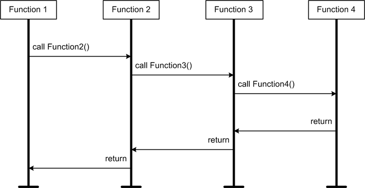
Actually, all software functions (and methods, too) can be
classified as either blocking or nonblocking, and the majority of
functions within a typical software application are of the blocking
variety—that is, they don’t return until the intended action is complete
or an error is detected. You can see this in the message sequence chart
(MSC) shown in Figure 11-9. Here we have
Function1() calling Function2(), which in turn calls Function3() and finally Function4(). The time required for Function1() to receive a response from
Function2() is dependent on how long
it takes for functions 2, 3, and 4 to complete their processing and
return. During this entire time, Function1() is blocked. (In an MSC diagram,
events in a function or process occur in a top-to-bottom order, and
transactions between functions or processes are the horizontal
lines.)
Blocking allows functions to maintain synchronization and honor the intended flow of execution through the code. The action or data that the call is requesting may or may not be available at the time the call is made, so a blocking call will wait for the other end to respond in some fashion before returning to the caller. As a side effect, it will also effectively suspend your application until it returns.
The type of blocking we’re most interested in is when an application process is forced to wait for an interface, which in turn waits for a hardware device to respond. This is shown in Figure 11-10. Notice that there is a timer symbol in this diagram. This means that if the hardware does not respond within some preset period of time, the interface process will terminate and return an error.
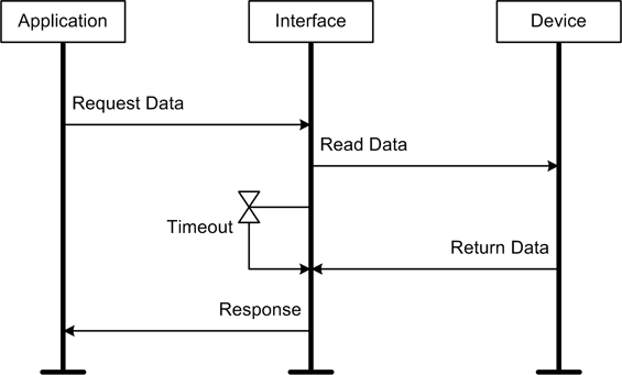
In some cases it may not matter if a blocking call waits for a bit before returning to the caller, and allowing this is more convenient than writing the necessary code to support continual query and retry actions. But, there is a warning in order here: when working with I/O devices, a blocking call without a timeout of some sort can potentially hang forever. This is usually a bad thing, and often the only way to get out of the situation is to shut down Python and restart the application. If your code is running on an unattended machine somewhere in the middle of nowhere, a fault that hangs a blocking call can be really, really bad.
One way to deal with this is to use nonblocking function calls. This entails some additional code, but it’s very useful when dealing with network communications and data acquisition. We’ll look at some ways to use this approach shortly.
Data I/O Methods
Now that we’ve seen what blocking and nonblocking functions entail, let’s look at how these concepts are involved with various operational modes of interface I/O. We’ll start with the simplest form, on-demand I/O, then proceed to polled I/O, and finally take a quick a look at multithreaded I/O.
On-demand data I/O
As I stated earlier, the two most obvious ways to move data into or out of your application are just a matter of reading from or writing to a port or device. When sending (writing) data using a serial (RS-232 or RS-485) or GPIB-type interface, there usually is no need to worry about the use of a blocking call. In the case of an RS-232 interface that does not use hardware handshaking, the data is sent out through the hardware port immediately. An RS-485 interface with a single master and multiple listeners should never block on a write by the master device, but the listeners may be unresponsive for a period of time. GPIB can also get into a situation where there are no listeners responding to the sender, but most GPIB interface APIs and the associated hardware can detect this and return an error code. Writing to a hardware interface API for a device such as a PCI interface card is usually not a problem in terms of blocking, but the call might still return an error code if something is amiss.
If your software uses on-demand calls to read data, they should be blocking calls, and your software should always check the return codes. If timeout parameters are available for a blocking function call they should definitely be used, but not every API provides blocking calls with timeouts (perhaps it was assumed that a timeout couldn’t possibly happen). For those situations you’ll need to use a nonblocking version of the API function and employ a different approach to implement a timeout in your own software.
Polled data I/O
A nonblocking call will return immediately, and its return code or return value will (hopefully) let the caller know whether or not it succeeded. A nonblocking call can be used to avoid an I/O hang, but it requires more code to support it. For example, let’s assume that the API we’re using has both blocking and nonblocking versions of I/O functions to read data from a device, or perhaps that the I/O functions have a parameter that can be set to control blocking. You can then put a nonblocking call into a loop that also checks for a timeout, like this:
def GetData(port_num, tmax=5.0):
    checking = True
    tstart = time.time()
    while checking:
        rc, data = ReadNonBlocking()
        if rc == ERR:
            break
        if time.time() - tstart > tmax:
            checking = False
            rc = TIMEOUT
        else:
            time.sleep(0.05)    # wait 50 ms between checks

    return rc, data
This is an example of polling: this function will attempt to get
data from a specific data acquisition device by continually polling
the port (using the ReadNonBlocking() function call) until valid
data appears. In between each read attempt it will sleep for 50
milliseconds. The delay is mainly for the benefit of the device being
read, as many devices can’t tolerate being hammered continuously for
data.
In order to actually have a polling function that doesn’t cause the rest of an application to suspend while it’s active, you need to use a thread.
Acquiring data using a thread
So far we’ve looked at on-demand and polled data I/O. Now let’s take a quick look at how we might check for incoming data without bogging down the entire system in a continuous polling loop.
There are two API functions in the following skeleton example
that we haven’t seen before: SendTrigger() and GetData(). It is assumed that these exist as
part of the API for the data acquisition hardware, and they do what
their names imply. Also, the type of data being acquired isn’t
specified, primarily because it doesn’t really matter for this
example. It could be anything, just so long as the specified number of
samples are acquired and no errors occur:
class AcqData:
    def __init__(self, port_num, timeout):
        self.timeout = timeout
        self.dataport = port_num
        self.dvals = []        # list for acquired data values
        self.dsamps = 0        # number of values actually read
        self.get_rc = 0        # 0 is OK, negative value is an error
        self.get_done = False  # True if thread is finished


    def Trigger(self):
        SendTrigger(self.dataport)


    def _get_data(self, numsamples):
        cnt = 0
        acqfail = False

        while not acqfail:
            self.get_rc, dataval = GetData(self.dataport, self.timeout)
            if self.get_rc == OK:
                self.datasamps = cnt + 1
                self.dvals.append(datavalue)

                cnt += 1
                if cnt > numsamples:
                    break
            else:
                acqfail = True
        self.get_done = True


    def StartDataSamples(self, samplecnt):
        try:
            acq_thread = threading.Thread(target=self._get_data, args=(samplecnt))
            acq_thread.start()

            self.Trigger()       # start the data acquisition

        except Exception, e:
            print "Acquire fault: %s" % str(e)

    def GetDataSamples(self):
        if self.get_done == True:
            return (get_rc, self.dsmaps, self.dvals)
        else:
            return (NOT_DONE, 0, 0)
This bit of code uses a thread, in the form of the function
_get_data(), to continuously read
the external device to obtain some number of data samples. Notice that
the hypothetical API function GetData() supports the use of a timeout parameter, and we can assume that it
will return an error code if a timeout does occur.
The key things in this simple example are how the thread is
created, and how we can check to see if the data acquisition is
complete. Python’s threading library includes a thread object method
called join(), which accepts an optional timeout parameter and is typically used to
block the execution of one thread while it is waiting for another to
complete. In this case we won’t use join(), so the thread is allowed to run on
its own. The accessor function GetDataSamples() checks the variable
self.get_done to determine if the
thread has finished. If so, GetDataSamples() will return the data
collected. If the thread is still running, it will return a 3-tuple
with the first item set to NOT_DONE. It is up to the caller to
determine if the sample count returned matches the sample count
requested.
This is just one way to do this, but it illustrates a
fundamental issue that is often encountered when working with threads;
namely, at what point does the program come to a halt and wait for
something else to finish what it’s doing? In a program that is designed to run
continuously, this can be dealt with by placing the call to
GetDataSamples() in a
single main loop in the application. This allows it to be checked
each time through the loop if data is expected, with the
results read back if they are available. Otherwise, the program could
just continue to use the last known results.
Handling Data I/O Errors
No matter how unlikely it may seem, errors can still happen, especially when dealing with interfaces to the real world. They might be the result of spurious noise on a serial interface, an out-of-range voltage level on an analog input, or a fault in an external instrument. How the software detects and handles errors is directly related to its robustness. Another way to put it would be to say that robust software tends to exhibit a high degree of fault tolerance.
For a system (be it software, hardware, or a combination of the two) to be called fault-tolerant implies that it has the ability to detect a fault condition, take action to correct or bypass the fault, and continue to function (perhaps at a reduced level of functionality) instead of just crashing or abruptly halting. The ability to continue to function at reduced levels of capability in the presence of an increasing level of errors is called graceful degradation. Of course, if the errors continue to mount, at some point the system will eventually come to a halt, but the idea is that it will do so after giving ample notice and it will not do it in a catastrophic fashion.
The reality is that there are almost always faults, and most things will eventually break or wear out. How much planning you should do for the mostly likely faults and the resulting errors is largely down to how much of a problem a failure will create. It might be insignificant (just ignore it and move on), or it could be a really big deal (something might explode, catch fire, or otherwise fail to stop an impending disaster). If you’ve done your up-front planning, as discussed in Chapter 8, you should be able to identify the nastiest scenarios and give some thought to how your system might deal with them should they arise.
Classes of errors
Errors can be grouped into two broad categories: nonfatal and fatal. A nonfatal error might be something like an intermittent communications channel, perhaps due to noise or other perturbations in the medium, or someone’s foot occasionally kicking a connector under a desk. Depending on the speed of the system and the duration of the failure, it may be possible to continue operation without adverse effects until communications can be reestablished. Another example might be an instrument that occasionally does not respond in a timely fashion, for whatever reason. If the command or query can be retried successfully with no ill effect, the error could be considered nonfatal. (Note that nonfatal does not mean nonannoying!)
A fatal error is one that requires significant intervention if the system is to continue functioning. Lacking that, it will need to perform a complete shutdown. An example of a fatal error would be the loss of control for the primary DC power supply used in an experiment. Unless there is a backup supply available that can automatically take over, the system will need to shut down until the problem can be resolved. Another example might be the failure of the control system for the liquid nitrogen supply used for the sorption pumps on a vacuum chamber, perhaps due to a failure in the control interface electronics, or a failure in the command communications channel. In either case, the system will begin to lose vacuum and potentially damage things like ion gauges or sputter emitters. At the very least, the current activity should be stopped until the problem is resolved.
Error retry and system termination
Sometimes it may make sense to retry an operation if an error is detected, perhaps after altering a parameter to compensate for the error. While this might sound clever (and it can be), it’s not something that should be done without some serious consideration of the context, cause, and consequences of the error. Blithely attempting to retry a failed operation can sometimes cause serious damage.
The more error-detection and self-recovery capabilities one attempts to build into a system, the more complicated the system becomes. This is fairly obvious, to be sure, but what isn’t obvious is how that complexity will manifest, and the subsequent implications it might have, not only for a particular subsystem, but for the system as a whole. As complexity increases, so too does the chance of new defects being introduced. Increased complexity can also increase the number of possible execution paths in the software, some of which may be unintended.
Figure 11-11 shows a scheme for handling a data I/O error in a fault-tolerant fashion. While this approach may not be suitable for every application, it does show why robust or fault-tolerant software tends to be an order of magnitude (or more) more expensive to implement than something that just does the I/O operation and returns either pass or fail. This is particularly true when performing testing to verify the fault-tolerant behavior. In Figure 11-11, there are three possible paths that can be taken should an error occur. In addition to the I/O operation itself, each of these paths must be tested by simulating the I/O and the error context. This rigorous testing involves a lot of work, but if you need that level of robustness there really is no other way to achieve it.
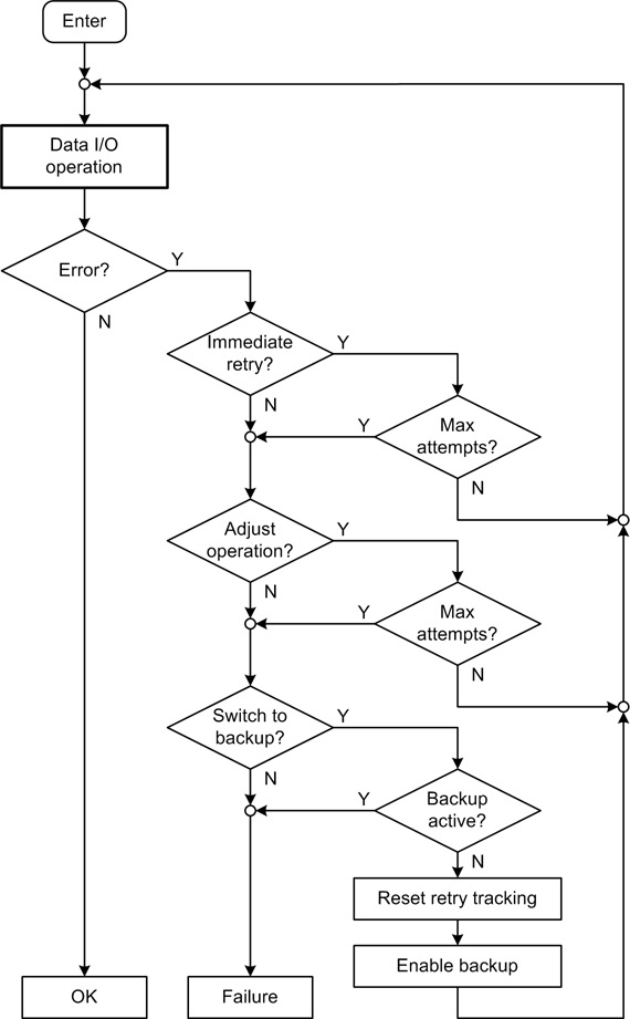
An interesting point to note about Figure 11-11 is the amount of
code it implies. The data I/O operation and its return code (pass or
fail, perhaps) are simple and straightforward, and might take no more
than a line or two of code to implement. With the error handling
included in the design, the code for performing a data I/O operation
will grow by anywhere from 10 to 100 times in size. This is typical of
fault-tolerant software. A large portion of it is concerned with error
detection and handling, and only a fraction actually deals directly
with the I/O. Also note that the last decision block, “Backup
active?,” means that if the backup is already in use (i.e., the test
is True), there are no more options
left except to fail.
When detecting and attempting to deal with an error, the system has to make a decision as to whether to attempt to recover from the error (and what recovery strategy to use) or just try to shut down gracefully. The logic making that decision must have inputs in the form of data describing the context in which the error occurred and the current state of the system, and there may also be a need to define excluded operations that should not be used.
For example, it may not be a good idea for a system controlling a pressure vessel to just relinquish control of the system without first performing some kind of check to determine if the pressure needs to be released. If the pressure continues to build even after the pumps and heaters are disabled (this can happen), there is a risk that the vessel may explode, especially if the error involved an over-pressure-related situation to start with. A graceful shutdown could possibly involve some type of venting action before control is completely terminated.
Similarly, if an error occurs in a system that is moving a mass of some type, does it make sense for the system to just stop? If the action of lifting or moving the mass entails control of power to a motor or servo, it might not be a good idea to just kill the power. The system may need to engage some type of braking or locking mechanism, or it might make sense for the mass to be lowered to a safe position prior to shutdown (if possible).
These considerations also come into play when attempting to retry a failed operation. Retries may not be appropriate after some types of failures, such as the loss of direct positional feedback, or the failure of a temperature sensor. Other failures may be known to be transient, and the operations can be retried some number of times before the situation is declared hopeless.
Consider the situation where the position of a secondary mechanism is dependent on the position of a primary mechanism, both of which are moving at a slow and relatively continuous rate for extended periods of time. The link between the two is a communications channel that is known to occasionally drop out due to system load or other factors. In a situation like this, the secondary mechanism that is following the primary one might be able to predict where it should be over short periods of time. This allows it to continue to function without an update from the primary mechanism. If after some period of time the communications with the primary mechanism cannot be reestablished, the secondary mechanism will enter an error condition. If it does reestablish the communications channel with the primary mechanism before the timeout period, it can update its position, if necessary, and reset the timeout.
Failure analysis, which we discussed briefly in the section Handling Errors and Faults in Chapter 8, comes into play when making decisions like these. If done correctly, it can provide the guidance needed to make the decision to terminate abruptly, terminate gracefully, or attempt to recover. Lacking a failure analysis, the best choice is often to just terminate gracefully, and provide sufficient information (typically in a crash log or something similar) to allow someone to go back and ascertain the cause of the problem later.
Error/warning message single-shot logic
It sometimes happens that something in a system will occasionally generate a nonfatal error or warning message, and while you do want to know that the error has occurred, you probably don’t want to see the warning messages over and over again.
An example of this might be a high-speed data acquisition device that, depending on whatever else is going on, might miss a data acquisition operation every now and again. The author of the API library might have considered this to be bad, but you might not, especially if your software is clever enough to toss out a bad sample and simply try it again (as we just discussed). So long as your software is applying a timestamp to the data and there are no specific requirements that the data be acquired at precise intervals (having an accurate timestamp can help with this), you can often just ignore the error and try for another sample.
Here’s one way to handle this:
# somewhere in the module's global namespace, we define some control
# variables and assign initial values (these could also be object
# variables):

msglock   = False
errcnt    = 0
errcntmax = 9   # this will result in 10 counts before lockout

# And here is the function/method that does the actual data
# acquisition and error message lockout:

def grabData():
    global msglock, errcnt

    rc = Acquire()

    if rc != OK:
        if msglock == False:
            errcnt += 1
            if errcnt > errcntmax:
                print "ERROR: Data acquisition failed %d times" % (errcntmax + 1)
                msglock = True
    else:
        msglock = False
        errcnt  = 0

    return rc
The idea here is to not emit an error message unless some number
of consecutive errors have occurred. When errors occur back-to-back,
the variable errcnt will be
incremented. When it reaches a threshold count, an error message will
be printed, but it will only be printed once. The first nonerror
return from the Acquire() call will
reset the error count and the lockout variable, msglock.
It is also possible to put the error count and lockout logic into a separate function, but remember that a function or method call takes time, and if you have a need for speed it might make more sense not to try to encapsulate this functionality, but just to leave it as inline code.
Handling Inconsistent Data
When attempting to acquire data, you may occasionally run into a situation where the quantity being measured exhibits some type of instability. This often occurs with devices that need time to stabilize after power-on before they begin to provide consistent readings. In other cases, the values being measured are so small that just the inherent noise in the system can introduce significant errors into the data.
Waiting for stability
Sometimes an instrument or external device needs a period of time to stabilize before it will return valid data. If you happen to know what that time period is in advance, all you need to do, theoretically, is wait until it has elapsed before attempting to take a reading. However, if the time period is variable (perhaps due to changes in the ambient temperature of the operating environment), a deterministic timeout period cannot necessarily be relied upon.
Figure 11-12 shows how a series of measurements can be used to determine when an input is stable.
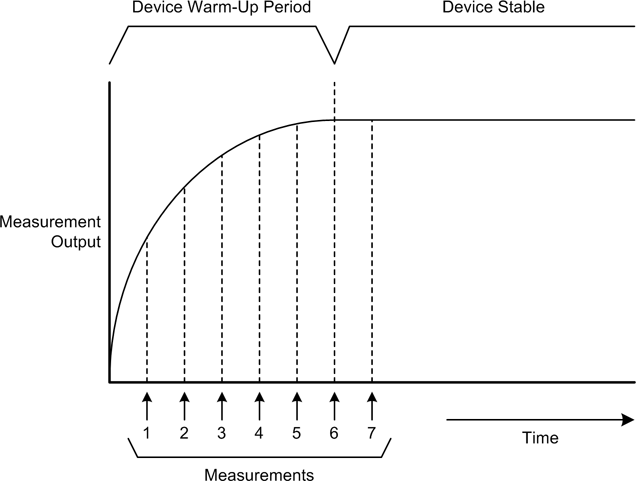
Depending on the inherent behavior of the instrument, the delta, or difference, between measurements may decrease as the instrument warms up, until it is close to zero. Hence, the difference between measurements 1 and 2 will be large, but it will be small (close to zero) between measurements 6 and 7. Due to noise or conversion errors, the delta may never be exactly zero.
In other cases the data may vary widely at first and then start to converge on a stable (more or less) output value, as shown in Figure 11-13. Precision solid-state laser controllers sometimes exhibit this type of behavior when attempting to measure the wavelength of the output beam. Until the controller and the laser head have both achieved an optimal operating temperature, the wavelength and the power of the beam may jump around, sometimes considerably.

The delta test function shown earlier (in the section Writing data) is a good candidate for checking warm-up stability convergence. A little additional logic could be used to set the delta match acceptance to something like two or three consecutive readings within tolerance.
The warm-up read and test approach offers a notable advantage over a simple timed wait in terms of fault detection. By taking a series of test readings and examining the delta between them, it is possible to determine if the data source is actually becoming more stable, or if it is having a problem achieving a stable output within a reasonable period of time.
Dealing with noise: Averaging
Now, let’s consider Figure 11-14. This shows a series of measurements that appear to be bouncing around in a random fashion. Depending on the scale, this might look worse than it actually is, but nonetheless the readings are not stable. This is not an uncommon situation when dealing with analog data inputs, particularly if the intent is to obtain a precise measurement over a small variance range and there is noise in the system.
One way to deal with this is by averaging the inputs over some period of time. Here’s a simple function to compute the average of an incoming stream of data:
data_sum = 0
data_avg = 0
samp_cnt = 0

def sampAvg(data_val):
    global data_sum, data_avg, samp_cnt

    samp_cnt += 1
    data_sum += data_val
    data_avg = data_sum / samp_cnt

    return data_avg
The global variables data_sum, data_avg, and samp_cnt must be set to zero before this
function is called. For now, assume that there is a list called
dataset that will hold the incoming
data values after they’ve been averaged. Each call like this one will
acquire a sample, average it with the samples already acquired, and
append the new value to the list:
dataset.append(sampAvg(readInputData()))
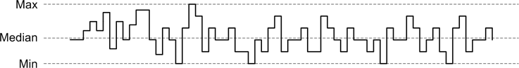
Averaging works best with data that is changing with each input sample. Figure 11-15 shows how averaging can help smooth out data that is fluctuating very rapidly.
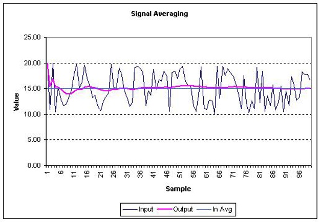
Of course, this isn’t real data (to produce data this nasty, something would have to be seriously wrong), but it shows how averaging fares with this type of input.
By the way, the averaging function used in this example is not optimal; it’s just there to illustrate one way of doing this. It would be better if the function calculated a continuous running average, so that there would be no need to worry about the summation variable eventually becoming a monstrous number.
Averaging can handle a lot of cases where data is changing on a small scale around a stable or very slowly changing mean, but it should be used with caution. An averaged signal that is trending either positive or negative will pull the average along with it, but if a change happens rapidly—say, a short-term variance that returns to the original level—the change will tend to be averaged out.
Summary
With the material that we’ve covered in this chapter, you should now have a good idea of what is involved when using an external instrument or device with Python, and the various tools that are available to help make everything work together. We’ve looked at serial, parallel, USB, GPIB, SCPI, and VISA interfaces, and at the basics of how one can implement an interface that is both robust and fault-tolerant. There are, of course, many deeper levels that we didn’t cover, but with what we’ve seen so far we can move forward into some working examples using real hardware.
Suggested Reading
In terms of books, USB is probably the most popular topic. With a little digging, you might be able to turn up a book or two dealing with RS-232 or RS-485. There really isn’t a whole lot available in the way of contemporary books about GPIB (or IEEE-488), but there are a lot of useful sources of information available via the Internet. Entering either “GPIB” or “IEEE-488” into Google will return numerous documents, some better than others.
Most of the books on Python that have already been referenced contain information concerning writing extensions in C or C++, and reviewing the API documentation for a particular piece of hardware is essential in order to use it effectively.
As a starting point, here are a few references you might find useful:
- Real Time Programming: Neglected Topics, 4th ed. Caxton C. Foster, Addison-Wesley, 1982.
Contains a brief but useful overview chapter on GPIB interfaces and the hardware handshaking GPIB employs. This book has long been out of print, but it is still possible to find used copies (also referenced in Chapter 9).
- USB Complete: The Developer’s Guide, 4th ed. Jan Axelson, Lakeview Research, 2009.
If you want to learn more about USB, you might want to consider this book. Axelson does a good job of explaining the low-level details of USB interfaces, with a particular focus on Human Interface Device (HID) class implementation. If you want to implement your own USB interface or just learn more about USB in general, this is a good place to start.
- http://www.ivifoundation.org/docs/SCPI-99.PDF
This link points to a PDF document that contains the complete SCPI specification. It is available free of charge through the IVI Foundation.
- http://www.ivifoundation.org/specifications/default.aspx
The IVI Foundation also has the VPP-4.3 VISA library reference available at no charge. If you’re going to use a VISA-compliant interface, you should have a copy of the documentation at hand.
- http://joule.ni.com/nidu/cds/view/p/id/852/lang/en
The NI-VISA 4.2 driver suite is available as an ISO file, ready to burn to CD. You can download it via this link.
The following semiconductor companies offer free application notes that cover a wide variety of topics of interest to instrumentation system implementers:
Analog Devices, Inc. (http://www.analog.com)
Maxim/Dallas Semiconductor (http://www.maxim-ic.com/appnotes10.cfm)
National Semiconductor (http://www.national.com/apnotes/)
Texas Instruments (http://www.ti.com)