
Chapter 14. Real World Examples
Beware of computer programmers who carry screwdrivers.
This chapter is intended to be a summarization of some of what I’ve presented in this book, so it’s not going to contain a lot of in-depth discussions. Rather than a step-by-step analysis and guide, it’s intended to be an inspiration for your own problem solving. You should be able to answer most questions that arise regarding the examples in this chapter by referring to the material we’ve covered in the preceding chapters, and if you need more details than can be found here you can look to the references and links provided in the chapters and the appendixes.
As you have probably surmised by this point, there are basically two main classes of instrumentation interfaces: those that require some type of add-on hardware that plugs into a computer, and those that require only a cable of some type. In this chapter we will wrap up our journey by examining examples of those devices that require only a cable. Drawing from what we’ve seen so far, we will see how RS-232 serial and USB interfaces can be used to acquire data and control devices in the real world.
We’ll start off with a data capture application for a DMM with a serial output (the same one we discussed briefly in Chapter 11), and then look at some other types of serial interface I/O devices that employ a more conventional command-response protocol. Next up is a USB data acquisition and control device, the LabJack U3. We’ll spend some time with the U3, mainly because it’s a complex device, but also because it’s typical of many devices of this type.
Serial Interfaces
When serial interfaces are mentioned, most people will think of RS-232, or perhaps RS-485. But in reality, a serial interface can take on a variety of forms. If, for example, we use a device to convert from USB to GPIB and back via a virtual serial port, we’re effectively using a serial interface, even though GPIB itself is a parallel data bus. The adapter and its USB driver perform what is called “serialization” of the data stream, so from the viewpoint of the software controlling or monitoring the device, it’s a conventional vanilla serial interface.
Serial interfaces based on RS-232 have the inherent advantage of being easy to work with, at least in terms of sending and receiving commands and data. Another aspect is that almost all instruments or devices with a serial interface use a command-response protocol. It is not that common to find instruments that will send data without being commanded to do so, but they do exist. One such exception is the tpi model 183 DMM, which we will look at next.
Simple DMM Data Capture
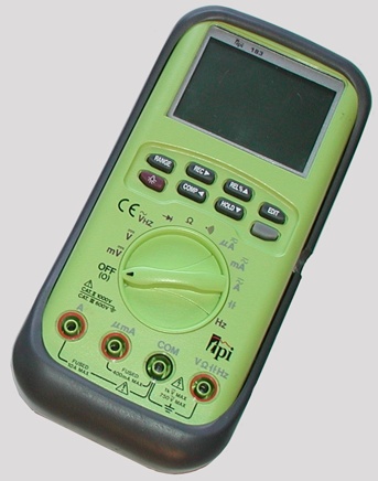
The tpi model 183 is an inexpensive DMM (around $130 from multiple distributors) with a variety of functions and reasonably good accuracy. It also provides a serial port in the form of a 3.5 mm jack and can continuously output a stream of ASCII data at 1,200 baud. If you connect the optional interface cable for the meter to a PC, you can capture this data and display it or save it to a logfile. Figure 14-1 shows the 183. The RS-232 interface is located on the righthand side of the case.
Note
There is a version of the 183, known as the 183A, that uses a different interface. This discussion is relevant to the original 183, not the 183A.
To start the RS-232 output, you hold down the “COMP” button while turning on the meter by rotating the dial. When the serial output is active the meter’s automatic power-off feature is disabled, so it can eat up a battery in short order. There is no provision for an external power source, so it’s not a good candidate if you need to leave it running for extended periods of time.
A serial interface kit is available for the 183 that includes some sample software and a special RS-232 cable. The serial interface is optically isolated, so the cable brings in DC power to the optical isolator in the meter by tapping one of the RS-232 control lines on the PC’s serial port. The cable for the 183 includes some additional internal components, so a conventional RS-232 cable won’t work. If you have a notebook or netbook PC without a true RS-232 serial port you can use an RS-232–to–USB adapter and communicate via a virtual serial port, so long as the USB adapter is able to supply the necessary RS-232 control line voltage.
The 183 uses the format shown in Figure 14-2 to encode the meter function, range mode, range, and data value into an ASCII string.
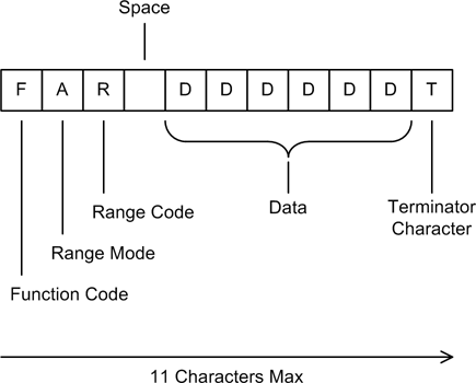
There are four distinct data items, or fields, and the function code field is actually hexadecimal. There are 11 possible values with one unused code, for a total of 12, so the numbering ranges from 0 to B.
Table 14-1 shows how to interpret the function code, and Table 14-2 shows the encoding used for the range codes.
Code | Function |
0 | AC volts |
1 | Ohms |
2 | DC volts |
3 | DC mV |
4 | AC amps |
5 | DC amps |
6 | Diode measurement |
7 | DC mA |
8 | Not assigned |
9 | AC mA |
A | Capacitance |
B | Frequency |
Function codes | Ranges | |||||
0 | 1 | 2 | 3 | 4 | 5 | |
0, 2 | 4.00 V | 40.00 V | 400.0 V | 1,000 V | – | – |
7, 9 | 40.00 MA | 400.0 MA | – | – | – | – |
4, 5 | 4.000 A | 10.00 A | – | – | – | – |
1 | 400.0 | 4.000 k | 40.00 k | 400.0 k | 4.000 M | 40.00 M |
B | 200.00 Hz | 2.0000 kHz | 20.000 kHz | 200.00 kHz | – | – |
A | 400.0n F | 4.000 μF | 40.00 μF | – | – | – |
3 | 400 mV | – | – | – | – | – |
6 | 4.000 V | – | – | – | – | – |
Now that we know what to expect, the following Python code snippet
shows how easy it is to pull out the four fields (where instr is the data from the DMM):
fcode = instr[0]
mcode = instr[1]
rcode = instr[2]
data = instr[4:len(instr)-1]
The first three fields are always one character in length. The
last field is taken to be whatever lies between the space (at instr[3]) and the end of the string minus 1
(we don’t care about the terminator character). The string itself must
be longer than nine characters. Any time we get a string from the meter
with nine or fewer characters, it should be tossed out.
There are several routes we might take when writing an application to capture data from this meter, and two that come to mind immediately. One is to just wait in a loop for the meter and handle things like writing to a logfile or updating a display in between readings. The other is to employ a thread to get the incoming data and push it into a queue that a main loop can then pull out and write into some type of display (or save to a file). The first approach is the more straightforward to implement. While the second is more flexible, it is also slightly more difficult to implement.
It’s important to account for the fact that the strings sent by
the meter have no EOL character. Shortly after one string is finished,
another is transmitted. In this case the safest way to get the data is
to use pySerial’s read() method and fetch one character at a
time while looking for the terminator character. This is where the
string length limit I just mentioned comes into play: if the capture
application happens to start reading characters in the middle of a
string, it could still see the terminator character and attempt to
extract data from an incomplete string. There’s no way to know what the
meter’s output will look like when your application starts listening to
it, so it will need to synchronize with the meter. Ensuring that at
least 10 characters have been read and the terminator is present greatly
reduces the odds of getting invalid data.
The code for a simple script to read the data stream from a 183
DMM is shown here as read183dmm.py:
#!/usr/bin/python
# 183 DMM data capture example
#
# Simple demonstration of data acquistion from a DMM
#
# Source code from the book "Real World Instrumentation with Python"
# By J. M. Hughes, published by O'Reilly.

import serial

sport = serial.Serial()
sport.baudrate = 1200
sport.port = "com17"
sport.setTimeout(2) # give up after 5 seconds
sport.open()

instr = ""
fetch_data = True
short_count = 0
timeout_cnt = 0
maxtries = 5    # timeout = read timeout * maxtries

while fetch_data:
    getstr = True
    # input string read loop - get one character at a time from
    # the DMM to build up an input string

    while getstr:
        inchar = sport.read(1)
        if inchar == "":
            # reading nothing is a sign of a timeout
            print "%s timeout, count: %d" % (inchar, timeout_cnt)
            timeout_cnt += 1
            if timeout_cnt > maxtries:
                getstr = False
        else:
            # see if the terminator character was read, and if so
            # call this input string done
            if inchar == '&':
                getstr = False
            instr += inchar
            timeout_cnt = 0     # reset timeout counter

    # if timeout occurred, don't continue
    if timeout_cnt == 0:
        if len(instr) > 9:
            # chances of this being a valid string are good, so
            # pull out the data
            fcode = instr[0]
            mcode = instr[1]
            rcode = instr[2]
            data = instr[4:len(instr)-1]

            # actual display and/or logging code goes here
            # the print is just a placeholder for this example
            print "%1s %1s %1s ->  %s" % (fcode, mcode, rcode, data)

            # reset the short read counter
            short_count = 0
        else:
            # if we get repeated consecutive short strings,
            # there's a problem
            short_count += 1
            # if it happens 5 times in a row, terminate the
            # loop and exit the script
            if short_count > 5:
                fetch_data = False
        # in any case, clear the input string
        instr = ""
    else:
        # we get to here if a timeout occurred in the input string
        # read loop, so kill the main loop
        fetch_data = False

print "Data acquistion terminated"
read183dmm.py has no provision
for user input. It will terminate after a read timeout has occurred five
times consecutively, so to exit this all you need to do is either turn
off the DMM or pull the interface cable out of the jack. It will also
terminate if it receives five consecutive short strings (len(instr) < 10), which indicates a
communications problem.
You would probably want to replace the print following the field extraction
statements with something a bit more useful, such as the ability to save
the data to a file or get command input from the user. The threaded
technique we saw in Chapter 13 would work well
here for user input. Also, from what we’ve already seen in Chapter 13, it would be a straightforward task to
extend read183dmm.py with a nice
display. I’d suggest an ANSI display for this situation, although it
wouldn’t be that difficult to build a GUI for it if you really
wanted to.
Serial Interface Discrete and Analog Data I/O Devices
Writing data capture and control applications for serial interface devices is usually rather straightforward once you know the command-response protocol. The tpi 183 DMM is just one example, albeit an off-nominal one (it only sends data, and has no commands). The D1000 series data transmitters from Omega Engineering are another, more common, example. These devices are fairly typical of data acquisition modules that utilize a conventional serial interface to receive commands from a host controller PC and send back responses via a serial interface. I chose them for this section not because I prefer them over any other device of this class, but rather because they have a rich command set and a lot of functionality stuffed into a small package. They aren’t the least expensive serial data acquisition modules available, but like most of Omega’s products they are easy to use and ruggedly built, and I’ve yet to have one fail.
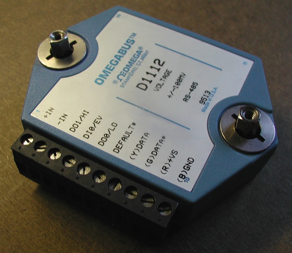
Figure 14-3 shows one member of the Omega D1000 series of digital data transmitters, which in this case happens to be a D1112. The analog input members of the D1000 family return data values from a sensor of some sort, typically a temperature sensor. They also have the ability to establish alarm set-points and scale the data, and some models provide extended discrete digital I/O capabilities.
The D1000 devices utilize a device addressing scheme as part of the command protocol, wherein the commands are prefixed with a device ID number, like so:
$1RD
The device will respond with something like this (depending on the input and the scaling):
*+00097.40
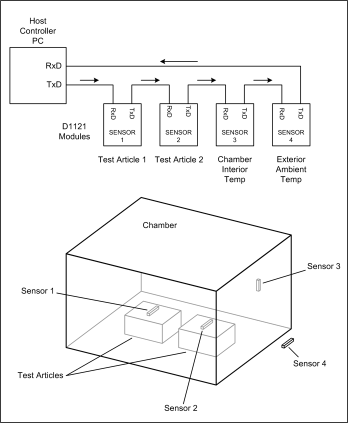
The device ID prefix allows multiple D1000 units to share a single RS-232 or RS-485 interface in a “daisy-chain” fashion. This is similar to the scheme described in Chapter 11 for RS-485 motor controllers. Figure 14-4 shows how several D1000-type devices can be used to monitor and control temperatures in a thermal chamber.
The setup shown in Figure 14-4 uses four sensors: two for the test articles in the chamber to prevent thermal damage, one for the chamber temperature, and one for the external ambient temperature. These could be thermocouples, thermistors, or resistive thermal device (RTD)–type sensors, so long as the input to the 1121 does not exceed 1 V (other models have different input voltage ranges). The devices labeled SENSOR 1 and SENSOR 2 are not used as control inputs to regulate chamber temperature, but rather as shutdown inputs should a test article exceed some preset temperature limit. SENSOR 3 would be the primary input to the temperature controller. The controller might use a bang-bang control, or it could use a PID algorithm, depending on how tightly the temperature needs to be regulated and the type of heating (and possibly cooling) system used with the chamber. SENSOR 4 is just an ambient external temperature sensor. Although it has no role to play in the operation of the chamber, data collected from this sensor could be used to determine how well the chamber is able maintain a specific temperature at different external ambient temperate levels. In other words, if the chamber is not well insulated and it is heating, the heating unit will work harder when the external temperature is low as it attempts to overcome heat loss from the chamber. By comparing the data from the external sensor with the internal temperature and the operation of the heating unit, we could work out an estimate of the insulation efficiency of the chamber.
For their small size, the D1000 modules pack in a considerable amount of functionality. The devices may be commanded to respond with two different string formats, which Omega calls short-form or long-form. Each module may also be assigned an identification string. One module might be “HEATER,” another might be “COOLER,” and so on.
All communication with a standard D1000 transmitter is of the command-response form. Unlike the tpi 183, a standard D1000 device will never initiate a conversation on its own (although it is possible to order them with this capability). A communications transaction is not considered to be complete until the D1000 has sent a response back to the host control system.
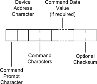
Figure 14-5 shows the layout of a
D1000 command. The command prompt character signals to the D1000 that a
command is inbound. The D1000 modules recognize four different prompt
characters, as shown in Table 14-3. The dollar sign ($) is the most common prompt, causing the
D1000 to return a short-form response. The pound sign, or hash (#), causes the D1000 to generate long-form
responses. The [ and ] prompts are used with the so-called Extended
Addressing mode, which I won’t go into here.
Prompt | Definition |
| Device returns short-form response |
| Device returns long-form response |
| Used with extended addressing |
| Used with extended addressing |
Following the prompt is a single device address character. D1000 devices are assigned an address by the user. Any printable ASCII character is acceptable as an address character, but in the interests of keeping things sane it’s a good idea to stick with the range 0 to 9, or perhaps 0 to F. Using address characters that don’t translate easily from a numeric sequence can make it awkward to use a loop to step through a set of daisy-chained devices.
After the address character come the device command characters, of which there may be two or three. Next is any parametric data the command might require. Some commands, such as query commands, do not require any additional data. Last, the command may use an optional two-character checksum, which is described in the D1000 user manual. Table 14-4 is a summary of the D1000 command set. For more details, including a discussion of each command and its nominal response, refer to the user manual.
Mnemonic | Definition | Short-form return |
DI | Read Alarms or Digital Inputs |
|
DO | Set Digital Outputs |
|
ND | New Data |
|
RD | Read Data |
|
RE | Read Event Counter |
|
REA | Read Extended Address |
|
RH | Read High Alarm Value |
|
RID | Read Identification |
|
RL | Read Low Alarm Value |
|
RPT | Read Pulse Transition |
|
RS | Read Setup |
|
RZ | Read Zero |
|
WE | Write Enable |
|
CA | Clear Alarms |
|
CE | Clear Events |
|
CZ | Clear Zero |
|
DA | Disable Alarms |
|
EA | Enable Alarms |
|
EC | Events Read & Clear |
|
HI | Set High Alarm Limit |
|
ID | Set Module Identification |
|
LO | Set Low Alarm Limit |
|
PT | Pulse Transition |
|
RR | Remote Reset |
|
SU | Setup Module |
|
SP | Set Setpoint |
|
TS | Trim Span |
|
TZ | Trim Zero |
|
WEA | Write Extended Address |
|
A D1000 response to a command begins with a prefix character,
followed by data, an error message, or nothing at all. There are two
possible response string prefixes: an asterisk (*) and a question mark (?). A third type of response scenario is when
the D1000 returns nothing at all, and a timeout condition is declared.
The asterisk indicates a no-error return, and a question mark indicates
an error condition. With error conditions, the question mark is followed
by the module ID, and then an error message. Here is a possible error
response to a command with an extra character:
$1RDX
?1 SYNTAX ERROR
Checking the response involves looking at the first character in the response string. If it’s an asterisk, all is well; otherwise, an error has occurred and must be handled. Analog data is returned as a nine-character string consisting of a sign character, five digits, a decimal point, and two digits for the fractional part. For example, the RD command will cause the device to respond with something like this:
*+00220.40
Conveniently, Python will accept the entire data value part of the string as-is and convert it to a float value, with no extra steps required.
Some commands do not return a data string in short-form mode, but all nonerror responses will return at least an asterisk character. The response for each command type is unique to that command (there’s no one-size-fits-all command response), so the software will need to be aware of what to expect from the device.
When dealing with devices like the D1000, especially if you find yourself working with them often, it might be worthwhile to create a class with a set of methods to handle the various functions. This is a lot cleaner and easier than the alternative of sprinkling the commands around in the code. It also allows for changes to be made in a single place (the class definition) and to take effect anywhere the class is used.
The Omega D1000 series devices are just one example of the kinds of products available for data I/O with a serial interface. There are many devices available for thermocouple inputs, RTD sensors, discrete digital I/O, and a mix of both analog and digital I/O. Entering the search strings “digital I/O RS-232” or “digital I/O RS-485” into Google will return hits for numerous vendors selling everything from kits to high-end devices for industrial applications. I would suggest that when shopping for serial interface I/O devices you make sure you’re not ordering a device intended for use with a DIN rail in an industrial setting. While there’s nothing wrong with these devices, the physical mounting requirements may prove more troublesome than something with just some plain mounting holes, and they tend to be more costly.
Serial Interfaces and Speed Considerations
RS-232‒based serial interfaces are typically rather slow, as RS-232 is limited to about 20 kbps, and that value starts to drop as cable length increases. RS-485 is much faster, with a maximum speed of 35 Mbps, and USB 2.0 can move data at a theoretical maximum of 480 Mbps. But the speed of the interface isn’t the whole story; there’s also the issue of how fast the software controlling the interface can send and receive the data.
For the types of applications described in this book a cyclic acquisition time of 10 ms (100 Hz) would be considered fast, and 100 Hz is well within the capability of Python running on a modern PC. However, update rates of 20 Hz are usually more than sufficient for many common data acquisition and control applications. Also remember that as the acquisition speed increases, so does the cost of the hardware and the complexity of the software.
The bottom line here is that there is absolutely nothing wrong with a device that uses a slow RS-232 serial interface for data acquisition or control, so long as it’s fast enough for the intended application. Here’s how we can do the math to see if a serial interface is fast enough.
Let’s say that we have a device with a 9,600-baud RS-232 interface. Each command is 8 bytes in length, and responses are a maximum of 10 bytes. There is a maximum 1 ms latency in the acquisition device between command and response (the latency is partly determined by the conversion time of the internal ADC in the device, and partly by the time required for any command or data processing between acquisition events).
At 9600 baud it will require about 8.3 ms to send a command from the host to the device, about 10.4 ms for the response to come back, and some time for the Python application to do something with it. If we add up all the times we might get about 21 ms for a complete command-convert-response-process transaction cycle. That works out to about 48 Hz. From this we can see that the serial interface transfer time dominates the acquisition rate of the device, which is typical for devices with slow serial interfaces. As the interface speed goes up, the time required for the command-response transaction becomes less of a limiting factor.
Although 48 Hz is usually more than fast enough for applications like thermal control, environmental monitoring, or stellar photometry, it may not be fast enough to acquire events such as pulses or other transient phenomena that might occur between the data acquisition events. Since the total cycle time of the control system is mostly the time involved in communicating with an external device or system, increasing the baud rate or switching to RS-485 are two ways to increase the speed and shorten the overall cycle time.
There is another way, however, and that is USB. In the next section we’ll see how to use a USB data acquisition and control device, which offers higher speeds and multifunction operation, albeit with slightly higher software complexity.
USB Example: The LabJack U3
Technological advancements in USB devices have continued to drive the cost of I/O devices with a USB interface ever lower. Just five years ago devices with the capabilities of this new breed of I/O modules would have cost many hundreds or even thousands of dollars. Prices today range from around $100 and up, depending on factors such as speed, conversion resolution, and the type and quantity of I/O channels.
One low-cost device is the LabJack U3, which is shown in Figure 14-6. This data acquisition device provides discrete digital I/O, analog I/O, and counter/timer I/O. It uses a USB interface for all command and data response transactions.
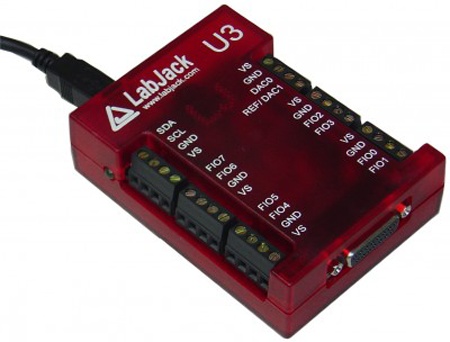
The U3 is powered from the USB interface. There is no provision for an external power supply, which is common for devices of this type. So even though there is +5 V DC available at some of the terminal positions, care should be taken not to draw too much current and cause the USB channel to go into shutdown.
LabJack Connections
Figure 14-7 shows a diagram of the U3’s connections. Many of the terminal points on the U3 can be configured for different modes of operation, and the configuration can be saved to ensure that the unit starts in the correct state at power-up. In addition to the terminal block connections, there is also a DB-15 connector that brings out 12 additional signal lines.
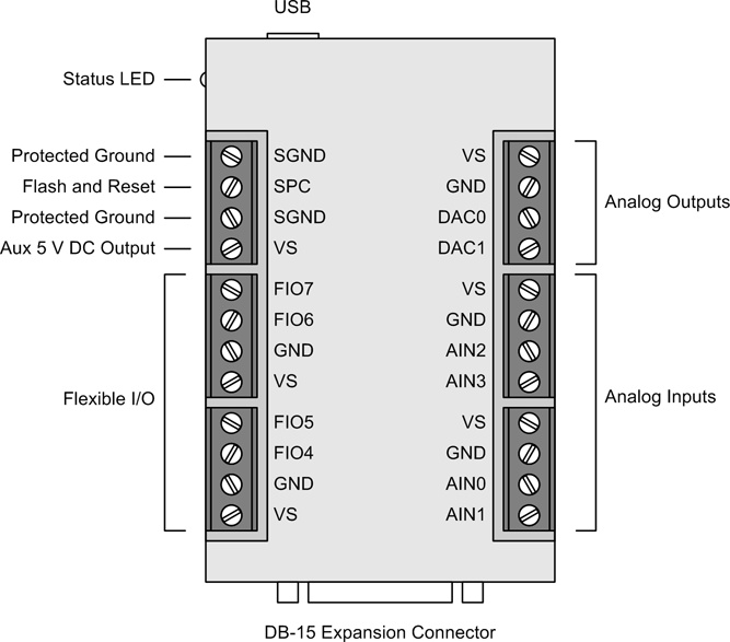
You can connect more than one LabJack at a time to a PC by using USB hubs, but keep in mind that the increase in data traffic can result in slower response times for all connected devices.
The LabJack U3 provides eight FIO (Flexible I/O) ports on the terminal blocks, and eight EIO (Extended I/O) ports and four CIO (Control I/O) ports on the DB-15 connector. In addition, there are two DAC outputs, six VS (+5 V DC) terminals, five common ground terminals, and two protected ground terminals. Notice that the terminals labeled AIN0 through AIN3 are actually FIO ports FIO0 through FIO3. These are configured as analog inputs by default, but you can change their function by modifying the LabJack’s configuration. You can use the LJControlPanel tool for Windows (supplied with each LabJack) for this purpose, or you can set the device configuration using the interface driver commands.
With the exception of the U3-HV model, each FIO and EIO port may be configured as a digital input, a digital output, or an analog input. On the HV version of the U3 the lines FIO0 through FIO3 are set as analog inputs and cannot be reconfigured. The four CIO lines on the DB-15 connector are dedicated digital lines.
The two DAC outputs operate in either 8-bit or 16-bit mode with a range of between about 0.04 and 4.95 volts. Using the 8-bit mode may result in a more stable output with less noise.
The U3 contains two timers and two clocks. Whenever a timer or clock is enabled, it will take over an FIO channel. In the U3-HV FIO4 is first, followed by FIO5, and so on. The standard U3 starts the counter/timer assignment at FIO0.
Installing a LabJack Device
LabJack supplies drivers for both Windows and Linux, as well as a complete Python interface wrapper. First we’ll take a brief look at what is involved in getting a LabJack device installed and running on either a Windows or Linux machine—it’s very easy, actually. In the next section we’ll dig into LabJack’s Python interface.
LabJack on Windows
To use a LabJack device with a Windows system, you need to install the UD driver supplied on the CD that comes with the LabJack unit. Install the driver before you connect the LabJack to your computer. Each LabJack DAQ device includes a single-sheet set of quick-start instructions that help make the whole process quick and painless.
LabJack on Linux
To use a LabJack device with a Linux system, you will need to first install the Exodriver package from LabJack. The Exodriver is supplied in source form and the only dependency requirement is the libUSB library. On most modern Linux systems this should already be present, but if not it can be easily installed using a package manager. You will, of course, also need a C compiler (since gcc comes with most Linux distributions, this should not be an issue).
Building the driver should just be a matter of typing make and, if it’s successful, make install. You’ll need to be
root (or use sudo) to do the
install step. The LabJack website contains detailed directions at
http://labjack.com/support/linux-and-mac-os-x-drivers.
LabJack and Python
The Python interface for LabJack devices, called LabJackPython, is a wrapper for the UD and
Exodriver low-level interfaces. It allows access to the driver
functions, and it supports both Modbus register-based commands and the
low-level functions in the LabJack drivers.
Installing and testing LabJackPython
Once you have a LabJack device installed and running, you can download the Python wrapper and install it. You can get more information about the Python binding at http://labjack.com/support/labjackpython, including installation instructions.
In summary, all that you really need to do is download the latest LabJack Python file (in my case it was LabJackPython-7-20-2010.zip), unpack it, change into the src directory, and type in:
python setup.py installThat’s it. You should then be able to start Python and import the LabJack module, like so (if you have a U6, import that instead):
>>> import u3Next we need to create a new object of the U3 class, which will be used for subsequent
commands to the device:
>>> u3d = u3.U3()Provided that your LabJack is plugged in and ready, you should see nothing returned from this statement, and you’ll be ready to start entering commands and reading data.
LabJack driver structure
We’re now well out of the land of serial interface devices and deep into API territory, which means we will need to understand how the LabJack driver API is structured in order to use it effectively. Dealing with a device like the LabJack is very much like working with a bus-based device and its low-level drivers. There is a lot of functionality there, but it’s not quite as easy to get at as it is with something like the serial devices we saw earlier.
Before getting too deep into things, you should take a moment to
at least glance through the LabJack user’s guide. You should also have
the source files LabJackPython.py and u3.py (or u6.py, as the case may be) close at hand,
because you will need to refer to them from time to time.
The driver API for LabJack is organized as a series of layers,
starting with the Exodriver or UD driver and eventually culminating in
functionality tailored to a specific model of LabJack device. This is
illustrated in Figure 14-8, which also shows
the u12 interface, which is a standalone API that uses its own
hardware driver, liblabjackusb.so, but doesn’t use the
LabJackPython interface module. The
u12 is included in Figure 14-8 for completeness
only; in this section we will focus mainly on the u3.
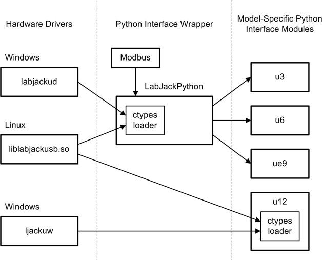
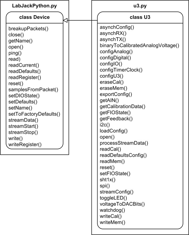
Our primary areas of interest are the LabJackPython.py module and the u3.py module. The u3 module contains the U3 class definition, which is a derived
class based on the Device class
found in LabJackPython. Figure 14-9 shows the inheritance relationship between the Device and U3 classes.
In addition to the Device and
U3 classes, there are also
functions in the LabJackPython and u3 modules that are very useful, but you
need to make sure that a particular function isn’t OS-specific. For
example, the ePut() and eGet() functions in LabJackPython.py are Windows-specific. If
you do elect to use these functions, bear in mind that your program
will no longer be portable.
In addition to the U3 class, there are functions and classes
available in the LabJackPython modules
that may be accessed without using the U3 class. For example, to get a
listing of U3-type devices connected to the system you can use the
listAll() function, like
this:
>>>import u3>>>u3.listAll(3)
The parameter value of 3
indicates that you want a list of U3 devices. For U6 devices you would
use a 6. In my case I get a
dictionary object in response that shows a single U3:
{320037071: {'devType': 3,
'serialNumber': 320037071,
'ipAddress': '0.0.0.0',
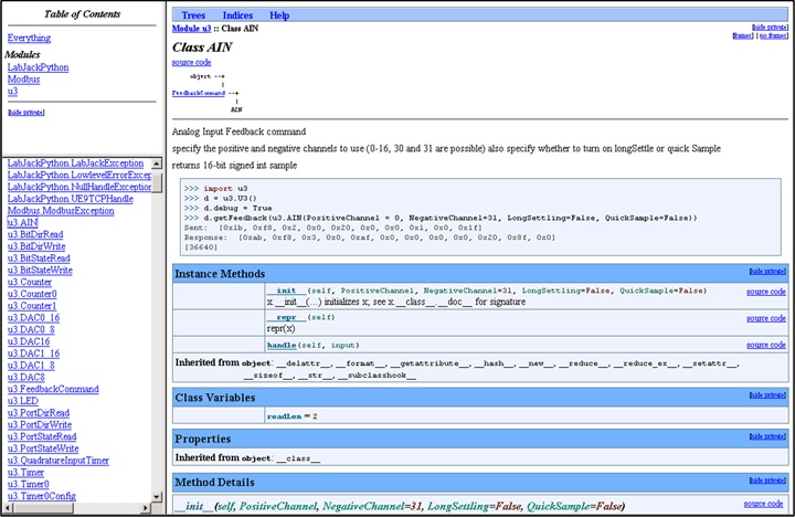
'localId': 1}}If you have Epydoc installed (see Chapter 8), I would suggest using it to create a
set of HTML pages as online documentation for the various Python
components. You’ll get nicely formatted documentation that is a lot
easier to read than using Python’s help() command or reading through the source
code. When used on the modules LabJackPython.py, Modbus.py, and u3.py, the output of Epydoc looks like the
screen capture in Figure 14-10.
U3 configuration
It is important to manage the configuration of a U3 device so
that the port definitions will be as expected for a particular
application when the device is powered on. The U3 class
provides the methods configIO(),
configAnalog(), configDigital(), configTimerClock(), and configU3() for this purpose. The sections Python API Types and Functions, The Method Table, and Method Flags of
the LabJack documentation describe the configuration management
methods. Here’s how to use configU3():
>>>import u3>>>u3d = u3.U3()>>>print u3d.configU3()
This returns a dictionary object. In my case the output looked like the following:
{'TimerClockConfig': 2, 'TimerClockDivisor': 256, 'LocalID': 1,
'SerialNumber': 320037071, 'CIOState': 0, 'TimerCounterMask': 64,
'DAC1Enable': 1, 'EIODirection': 0, 'DeviceName': 'U3-HV',
'FIODirection': 48, 'FirmwareVersion': '1.24', 'CIODirection': 0,
'DAC0': 0, 'DAC1': 0, 'EIOAnalog': 0, 'CompatibilityOptions': 0,
'EIOState': 0, 'HardwareVersion': '1.30', 'FIOAnalog': 15,
'VersionInfo': 18, 'FIOState': 0, 'BootloaderVersion': '0.27',
'ProductID': 3}
If you have access to a Windows machine, or you’re planning to use a LabJack with Windows, I would suggest using the LJControlPanel tool, at least until you get familiar with the configuration management methods and functions in the interface modules.
Using the Python interface with the getFeedback() method
If you’ve taken a peek at the u3.py module, you may have noticed that there are a number of little
class definitions in addition to the U3 class, each of which is derived from the
FeedbackCommand() class. (If you
haven’t done so yet, now would be a good time to take a look at this
module.) They are used to perform various operations in the context of
the getFeedback() method in the
U3 class.
Here is the definition for the getFeedback() method from the U3 class:
getFeedback(self, *commandlist)The parameter
commandlistis a list ofFeedbackCommand-type objects. The methodgetFeedback()forms the list into a packet and sends it to the U3.Returns a list with zero or more entries, one entry per object in the input list.
Here’s a simple example for controlling the status LED on the side of the U3:
>>>import u3>>>u3d = u3.U3()>>>u3d.getFeedback(u3.LED(0))[None] >>>u3d.getFeedback(u3.LED(1))[None]
To set the DAC output levels, you could do the following:
>>>u3d.getFeedback(u3.DAC16(Dac=0, Value = 0x7fff))[None] >>>u3d.getFeedback(u3.DAC16(Dac=1, Value = 0xffff))[None] >>>u3d.getFeedback(u3.DAC16(Dac=0, Value = 0x0))[None] >>>u3d.getFeedback(u3.DAC16(Dac=1, Value = 0x0))[None]
After entering the first two DAC commands, you should be able to
measure an output level of around 2.5 volts on DAC0’s output terminal,
and about 4.95 volts for DAC1 (0x7fff is half of 0xffff). The last two
commands set the DAC outputs back to zero. The getFeedback() method uses the u3.DAC16() function to send the value to the
DAC. Notice that the return value is None.
The following is a list of the FeedbackCommand derived class commands in the
u3.py module. For readability, I’ve
listed each class with the parameters passed to its __init__() method as if it was a function or
method:
AIN(PositiveChannel,NegativeChannel=31,LongSettling=False,QuickSample=False)WaitShort(Time)WaitLong(Time)LED(State)BitStateRead(IONumber)BitStateWrite(IONumber,State)BitDirRead(IONumber)BitDirWrite(IONumber,Direction)PortStateRead()PortStateWrite(State,WriteMask=[0xff, 0xff, 0xff])PortDirRead()PortDirWrite(Direction,WriteMask=[0xff, 0xff, 0xff])DAC8(Dac,Value)DAC0_8(Value)DAC1_8(Value)DAC16(Dac,Value)DAC0_16(Value)DAC1_16(Value)Timer(timer,UpdateReset=False,Value=0,Mode=None)Timer0(UpdateReset=False,Value=0,Mode=None)Timer1(UpdateReset=False,Value=0,Mode=None)QuadratureInputTimer(UpdateReset=False,Value=0)TimerStopInput1(UpdateReset=False,Value=0)TimerConfig(timer,TimerMode,Value=0)Timer0Config(TimerMode,Value=0)Timer1Config(TimerMode,Value=0)Counter(counter,Reset=False)Counter0(Reset=False)Counter1(Reset=False)
Although these will look like functions when used in your code,
they are actually class definitions that instantiate objects. It is
these objects that are invoked by the u3d.getFeedback() method to perform a
particular action or set of actions. Refer to the u3.py source code for descriptions (or the
Epydoc output, if you’ve already generated it). Also, after importing
the u3 module you can use Python’s
built-in help() facility, like
so:
>>>import u3>>>help(u3.WaitLong)
Now that we’ve seen what the getFeedback() method can do, let’s put it to
work. u3ledblink.py is a simple script that will blink the status
LED until the input voltage at the AIN0 terminal exceeds some preset
limit:
#!/usr/bin/python
# LabJack demonstration
#
# Blink the U3's status LED until the AIN0 input exceeds a limit value.
#
# Source code from the book "Real World Instrumentation with Python"
# By J. M. Hughes, published by O'Reilly.

import u3
import time

u3d = u3.U3()

LEDoff  = u3.LED(0)
LEDon   = u3.LED(1)
AINcmd  = u3.AIN(0, 31, False, False)

toggle = 0

while True:
    # blink the LED while looping
    if toggle == 0:
        u3d.getFeedback(LEDon)
        toggle = 1
    else:
        u3d.getFeedback(LEDoff)
        toggle = 0

    # getFeedback returns a list with a single element
    inval = u3d.getFeedback(AINcmd)[0]
    print inval
    if inval > 40000:
        break
    time.sleep(1)

u3d.getFeedback(LEDon)
print "Done."
Any voltage source with a range between 0 and 5 V DC will work as the input to AIN0. Touching a jumper wire between the AIN0 terminal and any of the VS terminals will also do the trick.
getFeedback() isn’t limited
to just one command at a time. You can stack up multiple commands.
Here’s an example where FIO4 (which is configured as a digital output
in my setup) is rapidly toggled on and off. It’s fast, and you’ll need
an oscilloscope if you want to see this activity:
>>>biton = u3.BitStateWrite(4,1)>>>bitoff = u3.BitStateWrite(4,0)>>>u3d.getFeedback(bitoff, biton, bitoff, biton, bitoff)
When using getFeedback() you
should bear in mind that some commands may take too long to respond
with the default timeout setting, and you’ll get an exception from the
driver. The WaitLong() class
command may look appealing, but it’s safer to just use Python’s
sleep() method instead of embedding
a delay in the middle of a command object list. Just remember to keep
things short and don’t pile too many command objects into getFeedback().
You now have enough information to start doing useful things
with a LabJack. We’ve only skimmed the tops of the waves, however, as
there is much more that the device can do. The user’s guide and the
LabJackPython source code contain
the information you will need to be able to use the more advanced
features.
Summary
The examples in this chapter are just a small sample of what is available in terms of instrumentation hardware, and of what can be done with Python to acquire data and control external devices. We didn’t discuss specific examples of GPIB or bus-based I/O, although these types of devices are used extensively in instrumentation systems. However, if you look back at Chapters 2, 7, and 11, these topics are covered there at length.
The devices discussed in this chapter were selected specifically to illustrate some shared concepts in the world of instrumentation hardware, such as the ubiquitous command-response paradigm. From this perspective a serial data acquisition device is similar in many ways to a GPIB device, and some lab instruments have the ability to communicate via a serial port while still using the SCPI model. The LabJack data acquisition devices employ a driver API and a Python interface layer that is very similar to what you might expect to find with a multifunction I/O card for the PCI bus. Once you understand the basic concepts behind the various interfaces, you’ll be well on your way to being able to deal with just about any kind of instrumentation device.
With a modest outlay you can convert almost any PC into a data acquisition and control system, and with Python you can program it to do what you want it to do and take advantage of the powerful and extensible Python development environment. Your programs can be as simple or as complex as you need them to be, and because it’s your software, you can modify it when you need to in order to keep up with changes in the requirements and the instrumentation environment.
If you’re comfortable with electronics you can even build your own I/O hardware, such as the parallel port interface we discussed in Chapter 11. You can also extend the capabilities of your system by incorporating networking and distributed control.
We’ve only just scratched the surface of what is possible. As you work with instrumentation devices and systems, more possibilities will begin to become apparent. Worthy candidates for some degree of automation are all around us in our labs and workshops, out on the production floor, in our vehicles, and in our offices and homes. With some practice, a little patience, and your creativity, you can apply the information in this book to design and build robust and elegant data acquisition and control systems to suit your specific needs.
Suggested Reading
The topics covered in this book are intended to provide you with the information you need to use the devices presented in this chapter. The primary sources of information for installing and programming devices such as data transmitters and DAQ units are, of course, the manuals supplied by the manufacturers. You should carefully read the documentation for a new device, as not all devices are intuitive or simple to use (very few are, actually). To that end, I’ve assembled a few links to online documents and other sources of information for the devices covered in this chapter:
- http://www.omega.com/DAS/pdf/D1000.pdf
An overview of the D1000 family of data transmitter products from Omega.
- http://www.omega.com/Manuals/manualpdf/M0662.pdf
The Omega D1000 series user’s manual.
- http://labjack.com
The source for the U3 and U6 LabJack devices, as well as the Python interface. The website contains application notes, a blog, and many other items of interest to LabJack users.