
Chapter 8
The Illusion of Space as an Element of Recording
Every record re-invents physics—the relationships and dimensions of our natural world. More precisely, space is redefined in every track to serve the recording’s artistic intentions. The physical positioning, relationships and the spatial qualities of sound and sound sources are presented in ways that cannot occur in the physical world, in ways that defy the basic principles of acoustics and physics and how we have experienced sound around us in real life. Sometimes these differences are subtle and other times they are pronounced, though their impacts on the track are profound; many of these percepts may not be apparent to the untrained listener. In records, there is an artistic use of space that serves, shapes and contributes substance to the track at all levels of perspective.
Spatial properties of the track play a dominant role in shaping the sound of the track as a whole and the sources it contains—a role shared with timbre. This connects fundamentally with two of the framework’s guiding principles: that every record is unique, and that of equivalence (each element has the potential to be significant, or contribute substantively at any time).
The significance of ecological perception in engaging recording elements was introduced in Chapter 6. Perhaps nowhere is it more profoundly in evidence than in the hearing of spatial properties. Research in psychoacoustics has offered much about sensations within the ear and its transformation of acoustic energy into neural impulses, but offers little in the way of information perceived and ‘heard’ (understood). Facets of ecological psychoacoustics (Neuhoff 2004a) and ecological listening (Clarke 2005) provide the concept of opportunities (affordances) for states of spatial properties and for their contributions to the track—and to listener interpretation. This is especially important for distance and environments, as we will discover. We hear spatial properties in context of the multidimensional layers of information within the track, not in isolation within a controlled laboratory. This distinction allows us to approach the properties of space as aesthetic variables; variables that can shape the track as much as any other. Thus, spatial properties open to the principle of equivalence.
Created (composed, invented) spatial qualities are integral to the individual track and the listener’s experience of it, and establish an individualized ‘reality’ for and ‘space’ of the record. They provide a sense of ‘place’ for each sound source, and a ‘stage’ for the ‘performance’ that is the track. Spatial properties bring the track to life for the listener; the listener accepts the virtual reality as part of the context and expression of the track—part of what makes it unique. This happens no matter the level of realism of the spatial properties.
This chapter will define the track’s spatial properties, and explore how they appear in and shape the record. It will navigate some of the ways we hear and perceive each spatial property, and engage in observing their attributes.
Before progressing with the spatial properties, however, we need to define the listener’s point of audition, and we need to examine initial challenges of hearing spatial properties of invisible sounds.
HEARING INVISIBLE SOUNDS IN VIRTUAL SPACE
Spatial properties are aesthetically central to the record’s content and its expression. This establishes a demand on our listening that most previous experiences have not prepared us to engage. Recorded popular music’s use of space (including amplified popular music performances) sets it apart from nearly all other music-listening experiences. Experiences that include visuals—such as motion pictures and video games—employ spatial properties, too, though rarely are they aesthetically central.1 In our everyday, casual listening our aural sense of space is not central to our experiences; it is a tangential quality that provides context or enhancement to the central focus—such as the sonic quality of a room around a speaker’s voice. When a spatial property arises and captures our attention, it is in the presence of visual experience. The aesthetic roles of spatial properties, and especially that we encounter the properties without the support of sight, further separates the record from real-world sound experiences.
When we engage space in everyday life, we process it as a multimodal experience. We bring sounds into our field of vision when they grab our attention; we open our eyes, and we turn our head or body toward the source. The geometry of a space is seen, in all its dimensions; our orientation to sources comes from looking at them; distance is estimated by sight much more than by sound; we turn our head to bring sources into the center of our vision to localize them. Vision takes over data collection; we quickly process and dispense with what was heard by shifting to fully engage and then define the experience with sight. Sound grabs our attention, but sight confirms the source. Sound may lead sight to discover and verify, as it provides the impetus that confirms physical relationships, though it does not provide the defining information in our daily life—for example, we look to identify a sound perceived as threatening. Sound may continue to contribute to the spatial experience, but it is typically the subordinate sense.
Listening to invisible sounds—to identify them or to localize them—is something we do not often attempt. When listening into the darkness, sounds in the night bring on imagining and often not knowing ‘what’s happening.’ Because we localize sounds and identify sounds so rarely by listening alone, we can feel confused or uncertain about what we hear.
We question ourselves: What is that sound? Where is that sound? What is it doing? Most typically, though, the sound is past tense—as ‘What was that sound?’ brings realization that our attention was elsewhere when the sound began. We wait, listening to hear the sound again to gain more information. We begin to question ourselves even more deeply: ‘Did I really hear that?’ We often do not trust our ears, our hearing—which is to say, what we perceived at the periphery of our attention and awareness. We experience a sense of uneasiness when relying on listening alone to figure out those things we cannot see—those things that go bump in the night. Acousmatic listening brings one to engage listening differently.
Clearly, real world listening leaves us inherently unskilled in engaging sounds without the aid of sight. Yet, this is exactly the context we find ourselves embracing with records. The track is wholly invisible, yet the track provides the illusion of spatial properties. Further, and very importantly, spatial properties provide significant substance to the record. Observing, recognizing and identifying spatial properties present challenges.
A reorienting of prior listening processes concerning space, a shift of attention toward sonic attributes previously not experienced, unknown or dismissed, and a sensitivity to the attributes that define spatial properties will each be required of the reader. It can present a challenge to hear what is now also unseen, to listen for the information of spatial attributes rather than allow the attributes to trigger sight. Sonic qualities never before experienced may be encountered by some. Finally, sonic qualities may need to be relearned or re-conceived to engage distance and angular orientation to the source; these may require reframing how to listen and what information to seek.
We search for a reference to make sense of the world around us. When listening to spatial properties in records, and hearing into its space (or spaces), the void of a visual reference can be disorienting. We may seek to use the only visual available: the loudspeakers. Those loudspeakers and their locations in the room will offer no guidance. Should loudspeakers be used as visual-to-sound reference they will mislead all percepts, except for the rare source located specifically at the speaker. Attempting to visualize sound locations by relationships to loudspeakers will mix two different contexts: the physical sound within the listening room and the virtual world within the track. Any common ground between the two will be by chance, and completely a coincidence of the particular track and the qualities of the physical room plus loudspeakers; observations will be distorted, and it is a distraction of effort to seek common ground. Further, sounds can appear at positions beyond the loudspeaker positions, extending the stereo array (see Figure 8.3).
Fortunately, we have inherent skills at hearing the attributes of direction, distance and environments that are capable of being developed (Blauert 1983, 47). These skills simply have not needed to be developed in our casual listening, and they can be honed to observe spatial properties within the track. Guided by clear understanding of the attributes that define spatial properties, we will use these skills for collecting information and for evaluating the track.
Listener Perspective and Track Playback Format
The listener’s perspective is used to calculate and define the spatial locations of sounds, and to understand the qualities of source host environments. An “implied physical perspective” (Williams 1980, 58) for the listener brings the impression of a point in space from which the track is heard; this is a vantage point from which listeners observe the track and its sounds. This conceptual location is the listener’s “point of audition”;2 this perspective is their perceived physical relationship to the track, that is defined as (or located at) a specific point in space. This term is adapted from film and television sound; I have transformed that definition to allow the term to identify and locate an unchanging listener’s position from which the track is observed.3
In everyday life, a point of audition is where one finds themselves at any moment; that position from which the direction and distance of sounds are perceived and unconsciously processed. Of course, as we navigate our lives our point of audition travels with us, and is continually changing with our moves of position. Here within recording analysis, though, we are concerned about this location more specifically; it is fixed throughout a track. The record establishes this position with its mix; the mix holds the assumption that the audience would hear the track from this same virtual position. This listener location needs to be recognized, and it needs to be stable in order to be of use for calculating sources positions and positional changes observed within the track. ‘Point of audition’ establishes a point of reference for calculating the angle and the span of space existing between listener location and sound source. The analyst will consciously process the qualities of space from one illusory physical location, a single point of audition. This defines the point of reference for all spatial calculations of the individual track; the point of audition is that point of reference, and establishes the listener perspective related to spatial properties.
Two-channel stereo (short for stereophonic sound) is the default format being addressed in all discussions; exceptions will clearly specify a different format such as surround sound (though ‘point of audition’ is also relevant to surround). This acknowledges the vast majority of music listening takes place using the two-channel version of a track; it is what nearly all consumers purchase and hear regularly. Indeed, the overwhelming majority of records are only available in two-channel stereo. Therefore, the spatial properties of stereo sound are integral to the vast majority of tracks.
Two other track formats are in common use: mono and surround. Either may be of interest to the analyst, and be examined in one’s analysis. All three playback formats will yield a different spatial experience. The three formats are:
- Stereo (with two independent channels)
- Surround sound (typically with 5 or 7 independent channels, with the potential for an additional channel that contains all of the lowest frequency range, which is directed to a subwoofer),
- Mono (a single channel containing all of the sound).
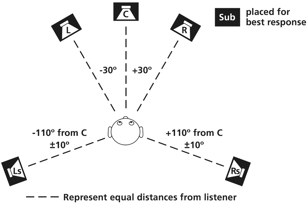
Figure 8.1 Left-right stereo loudspeaker configuration imbedded within the 5.1 surround sound layout recommended by the ITU (International Telecommunications Union); mono reproduced by center speaker or L/R stereo speakers.
Mono was the only format of early popular music recordings. Stereo (with its two independent channels) established a presence in the mid-1960s, and quickly dominated the market; initially two independent mixes were created: first for mono and an after-thought mix in stereo. Stereo is currently the default commercial format, and mono versions are now typically reductions of the stereo to a single channel. ‘Collapsed’ or ‘folded-down stereo’ merge the two channels of stereo into mono; this results in phase cancellations and other anomalies that alter the track, sometimes considerably. Mono records can be reproduced over two channel systems (sending the same information to both speakers producing “mirrored mono”) or over a single loudspeaker; these appear as either the center speaker of Figure 8.1 or the combined left plus right speakers. I have chosen to limit coverage of monaural versions of records primarily because of the overwhelming dominance of stereo in the literature. The spatial properties of mono are restricted to distance and depth, environments, and to a limited extent source size; Peter Doyle (2005) provides an extensive examination of spatial properties in mono tracks.
Stereo and surround sound playback formats locate sources very differently in relation to the point of audition. The listener is presented with sound arriving from different directions, different number of directions, and listening cues differ between the two formats, altering percepts. Each format provides a very different experience, with striking differences to source localizations, width and depth, and artistic treatments of sources; they shape the artistic statement of the track in very different ways.
The surround sound format, and all it brings to the track, will not receive coverage in this book. I have written about surround elsewhere (Moylan 2012, 2015, 2017); these provide a basis for recording analysis considerations that readers can pursue, though there is much left to be written. As surround sound continues to struggle for consumer acceptance and stereo substantially dominates over surround, it was decided not to engage it here. The format, however, has striking, distinguishing attributes not found in stereo; attributes that add substantive dimensions to the track’s aesthetics. The listening public has largely not experienced surround sound music production, but has embraced it for motion pictures. Perhaps these qualities may bring surround sound to become a more important part of the public’s music listening experience, just as home theatre sound has become widely embraced. For those of us who have experienced (let alone studied) surround recordings on a high quality system properly tuned, it is an experience that makes records new again—even tracks one knows well in stereo are rediscovered from their mix in surround.4
SPATIAL PROPERTIES AND ATTRIBUTES
Spatial properties and their attributes establish the sonic world of the track and a spatial identity for its sound sources. They can create “the appearance of a reality that could not actually exist—a pseudo-reality, created in synthetic space” (Moorefield 2005, xv), and they can provide a vivid real-life context for the track.
The track’s spatial properties present sounds in space where none are present. Sonic illusions locate sounds at direction and distance positions from the listener, and also provide sounds with size. Sounds may be localized anywhere within or around the listener’s listening field, at any conceivable depth and any angle reproducible by the playback format. Virtual spaces bring the experience of instruments and voices emanating from surreal rooms—illusions of rooms of any size, perhaps infinitesimally small or immensely large places, even spaces of impossible dimensions and geometry.
Curiously, perhaps astoundingly, the listener is perfectly willing to accept (albeit unconsciously) sounds emanating from these unknown, strange places. Worldly limitations are ignored, and listeners are willing to experience these illusions of distance and size, and accept them as the unique reality of the record. These qualities are wed to the fabric of the track, are an integral part of its sound and of its context; simply, they are part of the experience and substance of the recorded song. As such, the track may often be conceived as a performance emanating from a place of different sonic realities.5
The spatial properties of recording that establish these illusions fall into three categories:
- Angular direction and width
- Span of distance location and depth
- Dimensions of the environment within which an individual sound appears to be located ('host environment'), and dimensions of the overall environment the track occupies ('holistic environment')
This section will define the attributes of these three spatial properties in more detail, and discuss ways they interact, fuse, and work in complement. This is in preparation for a more detailed coverage of each that will fill this chapter.
Spatial Properties and Levels of Perspective
The dimensions of lateral angle (direction), distance, and illusory environments (simulated physical spaces) function most significantly on three (3) levels of perspective—levels we have already engaged:
- Individual sound sources and their attributes
- Composite texture of interrelationships of sound sources
- Overall sound
Table 8.1 adds detail to the three fundamental spatial properties, and how they manifest at levels of perspective.
Table 8.1 Spatial properties and their attributes or variables at the three levels of perspective.
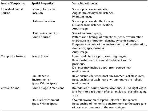
Listener attention naturally falls onto the perspective of the individual sound source. It is at this level that we interact with other humans, and at which we perform on instruments and sing. The perspective of the individual sound source represents the basic-level categorization; further detail of categorization brings more specific subordinate types (such as a particular performer or a type of guitar) (Zbikowski 2002, 31–33). Spatial properties shape the basic-level individual sound sources substantively; they add dimensionality. A spatial identity for each instrument, voice, or any other sound within the track results from (1) their left-right lateral placement, (2) their position of distance from the listener, and (3) the attributes of the individual host environment (space) they are perceived as occupying. The spatial identity is a virtual aural image of the source (1) having lateral location and size, (2) having distance from the listener, and (3) a sense of occupying a space that provides it with depth and a host room, space, or environment within which it exists and sounds.
These three properties are observed for each sound source at this perspective. The anomalies that establish environment and distance cues are at times much subtler than those of lateral sound location—both in real life and in the record. Sounds of environments can be pronounced though, and even incomplete sets of cues can establish illusions of physical, enclosed spaces. The perception of distance is fraught with misconceptions; distance attributes are often overlooked and confusion tends to replace distance with what is actually loudness, or reverb (an attribute of environments), or prominence, among others.
In the composite texture, sources are situated at a level of equal significance and are potentially balanced within the listener’s attention. This has been discussed earlier, and the concept continues for spatial properties. Here, individual sources are perceived in their interactions and relationships to other sources, and the interrelationships they might establish. The composite texture is where several important spatial traits manifest; these are based on the interrelationships of sound locations that coalesce on the sound stage.
In evaluating the sound stage, placements of sounds may establish groupings; the sounds dispersed across the stereo field and the depth of field can bond in various ways as a result of their timbral content, musical functions, staging placement, etc. Sources coalesce into groups within regions of the sound stage, and some may be isolated or delineated. This provides a connection or separation of sources and also of the materials they present; it also impacts the density of sound, and all that might entail.
Host environments of sources also establish relationships with the host environments of other sources, perhaps also generating percepts of distance and depth. Each instrument or voice might have its own ‘host environment’ (its own acoustic space, artificial room, reverb, etc.); relationships forming between instruments/voices are rarely akin to occurrences of naturalistic acoustic spaces. The sound stage houses rooms (spaces) that are positional in relation to other rooms—each containing a sound (instrument, voice), a performer, and an aesthetic idea. Each room (source host environment) is of its own geometry, size, sonic properties—real or surreal—and may change at any time. The sound stage has the potential to be active and dynamic, as well as contextual; in aggregate it establishes a context for the track, and much activity can exist within that framework without altering its fundamental context.
At the level of composite texture, the interaction of sources and spatial dimensions is evaluated. This contrasts with the spatial attributes of individual sound sources that are observed and evaluated at the track’s basic-level, above. Figure 8.2 illustrates these three perspectives: lateral and distance positioning of individual sound sources, composite staging of source image positions, and the placement of all sources within a holistic environment for the track. The identified sound stage width and depth can vary widely between tracks, as can the distance between the listener and the front edge of the sound stage.
At the highest level of perspective (the overall level of spatial properties), locations of all sounds coalesce into a single aggregate group. The grouping of sources establishes an area that is defined by width and distance—this area is the sound stage. This single all-inclusive ‘ensemble of sound sources’ resides within a single venue, a single space within which the track as an entirety resides—this is the track’s holistic environment. The holistic environment is an all-encompassing, global space or environment for the track; it also contains all of the track’s spatial properties that are generated from the individual sources and the sound stage—again, this aggregate is likely to be surreal.
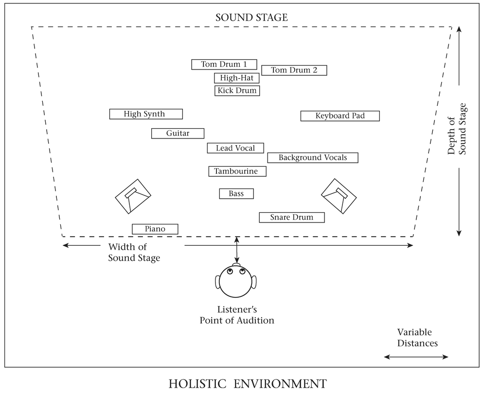
Figure 8.2 Sound sources positioned by lateral (stereo) location and distance from the listener, grouped into a single area or sound stage, which is contained within the track’s holistic environment.
In many genres of popular music or individual records, the listener experiences the illusion of a performance of the track; a performance that emanates from a single area that encompasses and binds all of the performers, and all of their sounds. This represents one conception of a sound stage for the track. The sound stage is positioned within an overall space that may also contain the listener’s position—the holistic environment, or the environment of the track, can be conceived as including the location of the listener, or detaching the listener as an observer. The holistic environment is at the highest level of perspective of all spatial properties; it contains all spatial properties. The sound stage and the holistic environment is contextual; they each establish a stable point of reference that may be used to understand lower-perspective activities. Some tracks are not staged performances, and others will not be conceived as performances by listeners; even in these situations, the sound stage can remain a helpful point of reference.
Elevation (the perception of sound located at an upward or downward angle along the listener’s median plane) has not become incorporated into stereo records, as the cues cannot be reliably or convincingly produced by two loudspeaker locations, on a common horizontal plane. For sounds at vertical angles to be consistently reproduced, an additional channel or channels of audio directed to a loudspeaker(s) located above and/or below the listener ear-level are required; these are found in the several emerging surround formats, with ceiling channels largely dedicated to environment cues. References to a vertical plane of the track typically refer to frequency or pitch register, or the ‘height’ frequency or pitch content: “All rock has strands at different vertical locations, where this represents their register” (A.F. Moore 2001, 121); rarely is activity on the vertical plane, situating sounds top to bottom, proposed (Hodgson 2010, 183–185). Neither of these references to the vertical plane is applicable to the discussions of this chapter.
In summary, the spatial properties of lateral placement, distance location and host environment are the basis for all that is space-related in the record. They have the potential to provide each instrument and voice with a unique spatial identity, and working together they establish the spatial identity of the track. These properties rely on the listener’s point of audition as a reference, allowing consistency to observations; the point of audition affords the performance of the record with some degree of separation from the listener, with sources at angles from the listening position and at some separation of distance, and with a sense of depth and other attributes from each source situated within its own performance space.
The following sections will present (1) stereo location of individual sources (in aggregate comprising the width of the sound stage) and (2) the distance location of sources (in aggregate comprising the depth of the sound stage). The sound stage (3) will be explored in detail afterward, before moving on to (4) the roles of environments in records, and their sound properties.
STEREO LOCATION: ANGULAR DIRECTION AND IMAGE WIDTH
Lateral (or stereo) location is the topic that arises when many think of a record’s spatial properties. It is the perceived lateral position of sound sources; their locations within the boundaries of the stereo array, calculated at an angle left or right from the listener’s forward facing center. Sound sources may be perceived at any lateral location within the stereo field, Figure 8.3. Sounds may be situated at either loudspeaker, though the majority of sound sources are located elsewhere, where no loudspeaker exists. “The stereo space acts as a sort of window through which the listener can ‘view’ the location of sounds. Not only in an overlapping construction but in a complex and dispersed structure” (Camilleri 2010, 201).
Illusions of sound placements can be established at positions where a physical source is not present. These illusions are produced by the interaction of the two independent stereo channels that emit from the two loudspeakers—speakers that are correctly positioned in relation to the point of audition—as each channel arrives asynchronously at both ears. Sound sources that appear without a physical presence are phantom images. The majority of sound images in nearly all stereo tracks are phantom images. Phantom images (and the sound sources they represent) may appear anywhere between the two loudspeakers, and up to 15° beyond (outside) each loudspeaker position.
Lateral placement of sounds establishes the width of the sound stage. The left-edge of the furthest left sound source image and right-edge of the furthest right sound source image define the sound stage lateral boundaries.
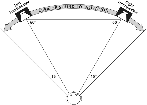
Figure 8.3 Stereo field: area of sound source localization in stereo.
Perception of Direction and Phantom Image Lateral Localization
Locating sound sources on the lateral plane relies on the perception of direction. Understanding a bit of the psychoacoustics for localization might assist the analyst in observing and assessing sources. In listening to the track, as in real life, the sound wave is different at each ear. These waves differ by time/phase, amplitude/intensity, and/or spectral content. These differences are essential to the perception of the direction of sound sources; they also play a role in the perception of environment attributes. Additional cues are required for the perception of distance and the attributes of spaces. Interaural cues provide decisive information for sound source location and angle on the horizontal plane, and for soundstage width.
The head, neck and shoulders act to produce time differences and intensity differences between the sound that arrives at each ear; these two types of interaural differences provide the primary cues used for perceiving direction. Jens Blauert (1983, xi) has noted the significance of sound at the two ears for perceiving spatial properties: “The acoustic signals presented to the two ears are by far the most important physical parameters of spatial hearing. It would be appropriate to discuss spatial hearing in terms of these signals alone. . . .” Handel (1993, 98) frames this a bit differently: “The human body acts to generate the physical cues for object localization. If we were only points in space with central ears, there would be no way to infer the direction of sound.” Direction of sound and locations of sounds are perceived largely through interaural differences of very similar waveforms.
Interaural time differences (ITD) are the result of the sound arriving at each ear at a different time; the physical separation of the two ears produce these differences. A sound wave will reach the ear nearest the source before it reaches the far ear. These arrival time differences also generate phase differences, as the wave at each ear has travelled a different distance; sound at each ear may be almost identical except the sound at each ear is at a different point in the waveform’s cycle (sound at each ear will also contain minute spectral differences) (ibid., 99).
Interaural amplitude differences (IAD) work in conjunction with ITD in the localization of the direction of the sound source. IAD are also identified as interaural intensity differences (IID). IAD is the result of sound pressure level differences at high frequencies present at the two ears. Reflections established by shadowing of the head, pinnae and upper torso produce interaural intensity (amplitude) differences at frequencies whose wavelength is shorter than the distance between the listeners two ears (frequencies above approximately 1600 Hz) (B. Moore 2013, 247–275). The human head acts as a low-pass filter (of sorts) where frequencies above approximately 2 kHz are attenuated at the ear opposite of the side where the signal originates (Mather 2016, 114). This disparity between 1600 and 2000 Hz as the approximate threshold for dominance of IAD percepts reflects the inconsistency of human physiology—as we each have a uniquely sized and shaped head, and each outer ear, hearing canal, inner ear (etc.) is different from the other and between individuals.
Interaural spectral differences (ISD) occur throughout the frequency range. While they may be subtle, they are important for the localization of objects in frequency ranges where IAD and ITD are ineffective. ISD are produced by the ridges of the pinna (outer ear); as sound reflects into the ear, the ridges introduce small time delays between their reflections and the direct sound that travels directly to the ear canal. Resonances also appear to be excited by, or produced within the outer ear. These also alter the frequency response of the sound source in predictable ways that vary between individuals. Important to recognize for surround sound, distance and location judgments are not as accurate to the sides and the rear. The absence of this spectral information generated from and collected by the outer ear seems to play a central role.
Pinnae serve a critical function in front to back localization. When sound arrives at the head from the rear, ridge reflections are not generated. When sounds are generated beyond 130° from the front center, pinnae block the rear-arriving direct sound from reaching the hearing canal and its ridges (Tan, et al., 2018, 40). The sound source is recognized as being present at our rear because of the absence of pinnae-generated spectral alterations (Mather 2016, 114).
Table 8.2 Interaural sound localization cues by frequency range.
With this information an analyst may direct attention to how specific interaural cues might be acting upon sound source placements. In doing so, one might most accurately identify the location of sounds by considering their prominent frequency content. Table 8.2 provides some guidance of which cue may be most appropriate for initial observations; the physiology of individuals brings frequency ranges and thresholds to vary slightly. This table is a point of departure for exploration, not a definitive guide. The nature of spectral content can bring localization of sources to manifest in unexpected ways. For example, a lower pitched sound (such as a bass) may localize more clearly than its presence well below 500 Hz might suggest; it might be localized by amplitude differences resulting from high-register frequency content in its attack, resulting in a narrower and more focused image than would result in other bass timbres. Localization typically occurs within the onset of a sound, bringing greater significance to this initial window of time; in real life we quickly determine where a sound is, then shift our attention to process other information (i.e. what it is doing, and whether it is necessary to react or take action).
There is no reason to believe we hear equally well in each ear, or that both ears share the same functional characteristics. We don’t see equally well with both eyes; we are comfortable in this knowledge, as the majority of us experience this regularly while being fitted with eye glasses. We do not have our hearing assessed regularly, and nearly all of us have no idea of how well our ears function in relation to ‘normal hearing.’ Given our physique is not fully symmetrical, and our outer ears are not identical and eye glasses need adjustments to conform to our head and ear location irregularities, it bears that we hear at least slightly differently in each ear. Further, we seem to have a dominant ear—anecdotal observations have proposed most people consistently put a phone up to the ear of their dominant hand, and others have proposed ‘creative’ people put their phone to their left ear. I offer no validation of these, as few formal studies have engaged ear dominance, or examined acuity imbalance except under trauma and restorative conditions. Anecdotally, though, it does appear many of us have a preferred ear we use to lean into a conversation, to talk on the phone, and so forth—just as we consistently make our first step off the bus with a certain foot, and stumble should we start with the other. Consider, you cup one ear (rather than the other) to hear more clearly. These matters of imbalance of hearing acuity between each ear and the possibility of a dominant ear have potential bearing on interaural perception—a bearing that is largely undefined.
This is a meaningful place to remember the explanation from Chapter 6 of how headphones present the spatial properties of tracks differently from loudspeaker listening—in ways that directly transform the spatial qualities being examined in this chapter. Headphones eliminate interaural cues and thereby establish voids in the stereo field where images cannot be formed (and those contained in the track reproduced); further, this establishes “an unnatural stereo image which does not have the expected sense of space and appears inside the head” (Rumsey 2001, 59); lastly, the closeness of the drivers to the ears exacerbates timbral detail, and alters distance and depth positions of sources and the timbres of environments. The sound stage and localization are wholly different experiences over headphones as compared to what is heard out of loudspeakers. The vast majority of records are created while listening over loudspeakers; the spatial properties generated by loudspeakers are integral to the sound established as the track’s finely crafted artistic statement (including recording elements); the sounds emanating from loudspeakers are integral to the track’s primary text.
In order to collect observations that accurately reflect the lateral characteristics of sounds, interaural cues need an accurate and consistent point of audition. Listener location at the apex of the equilateral triangle that defines the loudspeaker to listener position is critical; a shift of position brings a shift of angle/location of sources—even a small shift can make a substantial difference. This is a significant concern, as the positioning and sizes of sources are integral to the track; they play decisive roles in the spatial identities of individual sources and the track as a whole.
Image Width
Aural images (whether phantom images or located at a loudspeaker) also have a width dimension. This attribute is significant for the track, and it is often overlooked. Perhaps width does not get noticed because it is a quality rarely encountered in nature and life situations; when width then is present, we are ill-prepared to give it our attention. We are unaware of the presence of width, and do not have experience directing attention to that property. Further, its cues are typically subtle, though size can be perceived as more prominent when sounds are intimately close or when in highly reverberant spaces. Listening for width will be a new experience for many.
Width provides the illusion of a physical size to the sound source. Aural images have edges or boundaries on the left and right sides.6 They may be of any size width, spanning the extremes from occupying the entire breadth of the stereo field, to a very narrow point. Images may also change in width—at any time and by any amount. Subtle changes are common within instrumental or vocal lines, and more pronounced changes are common between song sections. Interesting examples of shifting image widths and positions give the sparse accompaniment of Phil Collins’ “In the Air Tonight” (1981) motion and direction, as well as suspense and tension, beginning with the first electric guitar sound.
Images that are very narrow in width, and clearly distinct as occupying a concentrated spot are point source images. Examples of point source images are not common. Sources in high frequency ranges produce point sources more readily, as these sounds tend to radiate less and be more directional. Lower frequency sources typically have resonant bodies that help the lower frequencies to radiate more, and thus provide the sounds with a sense of width. Paul Simon’s Graceland (1986) provides some interesting examples of point sources. Unusual point source electric guitar sounds are found in the opening riff to “Gumboots” and a similar guitar sound in the introduction of “Crazy Love, Vol. II.” Both sounds are near the center of the stereo field, and both are widened inconspicuously by reverb; each appearance has the guitar in a focused spot of direct sound, situated within a subtle and broader width of its space. More typical point sources appear in the collection of metal percussion sounds within the introduction and coda sections of “Under African Skies”; these sounds remain as focused points while shifting between lateral positions.
A spread image is one perceived to occupy a span of area; phantom images very often cover some expanse of width. The spread image is defined by the locations of its left and right boundaries (edges of the image), and by the area it is perceived to occupy. At times, a spread image may appear to be split, where it might occupy two more-or-less equal areas, one on either side on the stereo field. An example of a split image, polarized to each side of the sound stage, is the tambourine image during the first chorus of the Beatles’ “She Came in Through the Bathroom Window” (Abbey Road 1969, 1987).
In tracks, images are provided with width by the interaction of the two speakers each with different amplitude, timbre, and/or time-based characteristics of the source. The source is provided size by these differences between each channel. Width may also be the result of the attributes of a source’s host environment; the attributes of environment may produce an expansion of the edges of sounds. The sound of spaces may be prominent and distinct as a second presence, or may fuse with the source to create a blended sound.
Size is significant to stereo images, and contributes substance to their spatial identity. Sound source presence may be established and shaped by the amount of space they occupy; their prominence can be impacted by their size. As a result of their widths, images may overlap, occupy the same space, or be delineated in individuated areas; innumerable relationships are possible. When images are expanded by reverb or other environment cues, the edges of images that might otherwise be precise in their boundaries can acquire blurred and indistinct edges. This is significant, as images are defined by their size, as outlined by their edges; images with blurred edges take on different qualities, and may function differently in relation to other images.
These indistinct edges are established when an environment has a width greater than the sound source. This situation will typically also provide a sense of a different level of density (or amount of frequency present) within portions of the image. The central portion that is the source typically contains a greater level of substance than the edges (the environment). An example of these are the exposed drum sounds in the introduction to “The Boy in the Bubble,” also from Paul Simon’s Graceland.
Image size can bring unnatural qualities to a sound source, and unnatural relationships between sources. Imagine a flute occupying the entire breadth of the sound stage, and a piano confined to a single point in space. Width can have a strong impact on the aural image, and also on the realism of the track.
Sound Sources in Motion
Just as image sizes change, image locations are not fixed. It is as common for images to change in location as it is for them to change width. Images often move; they can abruptly change positions or gradually sweep to a new position. Abrupt changes in image location are common. They often shift positions between sections of the track, as mixes for verses and those for choruses can alternate throughout the track. Change can happen at any time, though, and sources may shift location by any amount along the entire stereo field. A change of position may be accompanied by a change of image width. Changes in position tend to be more readily noticed, as this skill is commonly used in daily life.
Actively moving sounds are not typical in tracks, but are certainly found. Moving sound sources may be of any width, travel at any speed, move to or between any locations. Narrow spread images and point sources most closely resemble our real-life experiences of moving objects, but the track is rarely governed by reality. Motion can be gauged by the amount of movement, or the difference between the starting and ending positions. For example, at the end of the introduction to Abbey Road’s “Here Comes the Sun” (1969) a Moog sound travels from the left loudspeaker to the center of the stereo field. The speed of movement, and the consistency of that speed represent other variables; here the sound moves steadily over the span of 4 beats. The image’s width remains stable throughout its motion.
Returning to Abbey Road, the lead vocal in “You Never Give Me Your Money” begins the song as a narrow image. It soon begins to gradually grow wider, until it occupies a significant portion of the stereo field; the sound’s environment contributes to this change with its gradual addition and varying qualities of cues and its changing proportion with the direct source sound. In the second section of the track, a new lead vocal sound gradually moves from the right to the left side of the sound stage; throughout the movement, the spread image maintains a similar size.
Motion between sounds may be present in a track. In this case a rhythmic structure can be established by interacting sounds located in different locations. The changing locations add spatialization to the rhythms, changes in timbres may also be present. Such occurrences are common in percussion parts, though examples between other instruments (especially instruments of the rhythm section) and voices (between lead and background locals) abound. Peter Gabriel’s “In Your Eyes” (1986) binds numerous percussion and drum sounds into a “spatialized rhythmic structure” (Théberge 1989, 104) that presents a strong rhythmic pattern between the instruments spread widely across the sound stage.
Observing Stereo Images
Data collection of source images can be engaged directly using the stereo location graph. Observations of sound source images—positions, size (width), and movements of size and locations—can all be notated on an X-Y graph. This image data can be clearly notated with as much precision as might be needed for the goal of the analysis; images can be located with great precision, or in a more general manner.
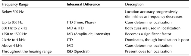
Figure 8.4 Calculating degree increments for stereo image source positions, and the vertical axis of the Stereo Location X-Y Graph.
The Y-axis positions the listener in the center, with the left loudspeaker location above and the right below the point of audition. This allows the listener to turn the graph to orient themselves at the point of audition. The axis is divided into degrees to the left or right of center, locating each speaker at 30˚ and the furthest left and right boundaries at 45˚. Figure 8.4 provides guidance in calculating degree increments on the stereo image graph.
Hearing Images
The challenge of hearing images successfully lies in accurately identifying their boundaries, or edges. As previously noted, in real life we do not directly engage the widths of sounds—and often they are not audible.
Beginning the process of hearing images, one is naturally drawn to the center of the image. This tendency is helpful to establish initial observations. With the eyes closed and head positioned correctly, one can readily point in the direction of the sound, to the core of its position;7 the skill can be refined with just a bit of practice. This will identify the general position or location of sources in the stereo field; the general distribution of sources might be assembled in this way, but the data would be quite incomplete.
Hearing edges of spread images requires focused attention. Once one has identified the center of the image, its edges can be sought. The point where an image begins can be elusive to start. It is one of the sound experiences of the track many have not previously experienced. Repeated listenings can reveal them through a process of guided exploration between ‘knowns.’
Knowing where the sound is not can assist one in identifying where it is. By directing attention outside the image, and gradually closing the point of attention toward the identified location one can make progress. The intention is to locate the edges of the image. By gradually closing the gap between where one knows the sound is and is not, one remains in control of the process. One can explore the material to find the point where sounds begin and end. Images with blurred, reverberant edges are a greater challenge, though this process will also help reveal their boundaries.
It will be obvious this skill is not as quickly honed as the general direction and positioning of sounds. It can be developed by attention and repetition, like most listening skills. This process of guided discovery—with guided attention alternating inside and outside the sound—will help significantly. As the attribute of image width and position are central aesthetic qualities of the track, engaging them can be crucial to meet the objectives of an analysis.
Using the Stereo Image Graph

Figure 8.5 Stereo imaging graph of “A Day in the Life” (1967, 1987). Graph contains two tiers of sources against the timeline.
Sources are placed on the graph according to the area they occupy. Edges of images are defined; the core of the sound occupies the space between them. Identifying the sources on the graph can be challenging without incorporating color or graphic patterns to fill the space between the edges. The graph can become unclear when numerous images are included, especially with wide spread images. In these situations, tiers can be stacked one above the other; this allows several groupings of sources (one on each tier) to be compared against the same timeline, as in Figure 8.5.
A suitable resolution to the timeline will be identified as observations progress; resolution is determined to clearly show the smallest degree of change the graph needs to clearly present.
The graph is capable of revealing considerable nuance of image positions, widths and their changes. Great detail may not be relevant to the goals of some analyses, though; in these instances, the Y-axis of the graph can be used without the detail of identifying positions by degree increments. The graph may also be dedicated to more general observations by changing the timeline resolution—perhaps to a level representing general positioning of particular sources within a section, rather than detailed positions and changes against a timeline.
Figure 8.5 contains two tiers of sound sources, following their activity throughout the first sections of “A Day in the Life” (1967, 1987). The Y-axis does not contain the detailed scale of degrees around the center, though the center position and left and right loudspeaker locations provide clear guidance of source locations and widths. The graph is the result of reducing a higher resolution version. Changes in image sizes are evident in the piano and acoustic guitar. John Lennon’s vocal gradually shifts across the stereo field, from right to left, over the duration of three verses and into the bridge; note several changes in width also appear. Percussion sounds have been omitted from the graph; these could be added to the graph overlaying the existing sounds, or placed on another tier.
Stereo Imaging Typology
Table 8.3 is a general listing of topics that could be collected in a typology table for stereo location. The table can be applied to data collection from X-Y graphs in a variety of ways—related to the number of sounds, the time area, and the variables under observation. For instance, a table might be dedicated to specific sounds within a specific section of the track; others might observe an attribute and its changing values of a single sound, of a collection of sounds, or of all sounds.
Table 8.3 Typology table attributes and values for stereo location images, and for the stereo field.


Multiple typology tables allow the analyst to focus on specific variables, attributes and sources, and to explore them in some depth. Typologies then may be compared and contrasted to gain a more holistic perspective and understanding. Separate tables for various structural sections of the track could be appropriate for many analyses that examine lateral placement of sound sources.
As in many other recording elements, the number of tables and their formatting is determined by the goals of an analysis—the type of information the analysis is seeking to explore and understand.
DISTANCE AND SOURCE POSITIONS IN THE TRACK
Distance is often misunderstood and misconceived, and therefore misperceived. Distance as a recording element is the amount of separation between the listener’s position and the position of a sound source. Framed differently: it is the degree of separation between the listener’s point of audition and the source’s location on the sound stage. We often confuse loudness for distance, amount of reverberation for distance, prominence for distance, and more; qualities that draw our attention can seem closer, something louder can create an impression of being closer than something softer, and an association such as a gentle breath can pull a vocal sound intimately close despite other contradictory distance cues. Distance perception is multidimensional and complicated.
Several important distance concepts shape the track: (1) the distance from the listener to the front of the sound stage, (2) the distance position of each individual sound source away from the listener, and (3) the distance placement of each sound source within its individual host environment.
The first two of these distances rely on the concept that the entire recording emanates from a single, holistic environment. This all-encompassing, global environment establishes a reference space for the track—a space within which the listener is also located. The listener position within the holistic environment is the point of audition—the listener’s position from which distance is calculated (and that was also used for calculating angle in lateral localization).
The stage-to-listener distance establishes the location of the front edge of the sound stage with respect to the listener. This is the distance between the closest source within the sound stage and the listener’s point of audition. This stage-to-listener distance also localizes the sound stage within the holistic environment of the recording, and provides a location for the listener inside the track’s overall environment. This distance plays a significant role in defining the listener’s level of connectedness to the track.
Each sound source is located at a more-or-less unique position away from the listener. These distances may be vastly different spans of space, ranging from unnaturally close to the listener to unimaginably far away. Distance positioning can differentiate sources from one another, as can lateral location and image size.
The depth of sound stage is the area occupied by the distances of all sound sources as they appear within their own host environments. The boundaries of sound stage depth are the nearest and the furthest sound sources—fused with the depths created by their environments, discussed below. The source’s host environment extends the sound source to have depth; this directly establishes depth to the sound stage. The perceived distances of sound sources within the sound stage may provide the illusion of great depth and a large area, the exact opposite of minimal depth and a minute area, or any state within a continuum between the two extremes.
Understanding Distance in the Track
Distance cues in the track are different from those in real life. This disparity—along with misconceptions about distance perception we may have often heard—is the source of many misunderstandings about distance in recordings, misunderstandings that result in misperceptions of source distances within the track.
In most of life’s contexts we first engage our prior perceptual experiences to understand what is newly encountered. In the track, what we have experienced for distance in the real world is often present for individual sources, as they are situated within their own environments—a very natural perception no matter the qualities of the environment. This is not the complete spatial identity of distance, though, and this partial presence serves to further confuse distance perception.
Within the track there are two distance cues: the distance placement of the sound source within its own host environment (just described) and the distance cue of the sound source in relation to the listener’s point of audition. It is this second percept—point of audition to source—that positions instruments and voices on the sound stage, and that is a dominant factor in distance perception in the track.
Let us briefly look ahead to examine Figure 8.10. Several sources are within their own performance spaces, the host environment within which they are located. These rooms and spaces place the sources within a sonic (virtual physical) presence at a specific distance within the sound stage. Note the sources are contained within their spaces; the listener is outside all spaces. The distance cues we have learned and rely upon for distance judgement are only useful within the spaces of the sound source; they are not fully in play in determining the placement of the sound away from the listener.
For distance localization in the track, timbral detail is the overriding attribute that defines a source’s position.8
In real life we hear the distance of sources within the spaces we occupy—whether enclosed spaces or free field spaces (out of doors, for example). We commonly rely on the cues of direct to reflected sound, of changing loudness and of spectrum changes when attempting to consciously judge distance—bringing mixed results. We process these cues, and sometimes they contribute to a reasonable estimation of distance position, and sometimes we make assumptions based on attributes that are not presenting distance cues. Our distance judgements are relatively inaccurate and our skills unrefined; we tend to rely on certain cues to make universal judgements about distance (especially loudness and reverberation), when those cues often have limited influence within a given context. Related to this, we have great difficulty judging the distance of sounds we do not know or cannot recognize.
Perception of Distance
Loudness is often considered a determinant of distance. A common notion is that louder sounds are closer sounds. Experiments have appeared to have born this out, but under certain test conditions that examine psychoacoustic perception without also investigating ecological and cognitive psychology (Neuhoff 2004b, 1–4). This is an important distinction. We often hear close, loud sounds in the world, and closer sounds may well be louder—at times. In music, a louder sound does not move toward the listener—neither in real-life acoustic performance nor in the track. A trumpet does not surge toward the listener during a crescendo. Louder is simply louder. In the track, loudness can increase markedly without adding the timbral detail that is gained when sounds move closer in the world.
As sounds move further from us, higher frequencies diminish more rapidly than lower frequencies—being absorbed by the air, attenuated by air friction. Timbral detail is diminished with increasing span of space between the source and the listener, and timbral detail is increasingly heightened with decreasing distance. Timbre is fixed when the source is recorded. Raising the amplitude level of a source in the mix does not change distance, when the changing loudness is not accompanied by a change of low-amplitude detail in timbre—loudness changes without timbral detail changes will not shift distance location. An increase in loudness might allow a sound’s timbral detail to be more apparent, in which case the timbral detail that establishes distance was made audible by the increased loudness—the loudness did not establish the shift, it revealed what was already present in the source. This is an important distinction for accurate localization of source distances.
While loudness and reverberation are often identified as “determinants” of distance, they are inconsistent and unreliable gauges of distance location and often not valid indicators. Loudness and reverberation are matters of coincidence and circumstance when they align with actual physical distance; these changes may be present because of changes of distance, and their qualities may reflect change in distance, but these are not causal. They are not directly transferred from one context to the next.
The ratio of direct to reflected sound and the time delay between direct and reflected sound may provide cues to distance within enclosed spaces. In the track, reflected sound (including echo) and reverberation are attributes of the space within which a sound is produced—its host environment. These create some confusion, as they may localize a source within an environment in the real world (this sonic experience suggests sources are in their own spaces contained within the space of the track itself, establishing a space within a space, discussed later). Still, a common misperception is to perceive a sound to be at a considerable distance, when presented with a sound appearing within a large environment containing a high percentage of reverberation. In the track, a sound can be placed intimately close to the listener while it is performing in an unnaturally enormous, overwhelmingly reverberant space—a space that contains the individual sound, a space that is then situated within the hierarchy of the holistic environment. Clearly, distance has several levels of dimension in the track.
Distance is very easily confused with other sound qualities. Perhaps this is because we have such little experience identifying the span that separates us from a source by sound alone. Sound elements are tangential to the visual (Schnupp, et al., 2012 177–189), so those sound elements that are prominent or are easiest to recognize (such as reverb or loudness) take over our perception—we seek to make them fit our experiences. For example, we equate loud with close, and highly reverberant with far, when the real world provides vivid experiences of close sounds in highly reverberant environments (singing in bathrooms?) and distant loud sounds (crack of thunder?). Handel (1993, 183) notes: “Listening is ‘making sense,’ trying to come up with the simplest and most plausible percept.” It ‘makes sense’ to us: if its loud then its near. It is helpful to remember what seems simplest and plausible may be a misinterpretation, a misperception, or misdirected attention. Schnupp, et al. (2012 188) contrasts loudness and visual perceptions related to distance to clarify this matter:
Obviously, we readily recognize distance positions of the known visual source; we are practiced at judging how visual objects change, decreasing in size proportionally as distance increases. We are not as skilled with recognizing the attributes of the sound that diminish with increasing distance—or that gain in resolution as distance decreases; instead we apply what ‘makes sense’ and cease searching for ‘what is.’
The dichotomy between the distance position of the source within its own space, and the distance of the source within the track can be a confusing one. It might be clarified with a central focus on timbral detail. Listening with attention on the level of subtle detail within a source’s timbre provides the cue to sound source position with respect to the point of audition.
Fortunately, we have the capacity to improve distance perception by bringing attention to a sound’s physical content. We locate sounds in distance by timbral detail, by observing the content of the sound. Also, we personally and culturally sense into distance of sources as they relate to personal space, bringing us to define our place and relationship to sources as they are situated in their location (more on this below).
A significant study of distance perception performed by Mark Gardner (1969) is often referenced and used to explain the perceptual process.9 Gardner’s study asked listeners to judge distance for shouted, normal and whispered voices; test subjects readily and accurately identified general locations and changes of distance from these sources, aided by instructions. Subjects also identified similar distance changes when presented with these sounds produced from the same location and at the same sound pressure; whispers were identified as closest, shouts as farthest. Examining this from experiential and ecological perspectives we might understand the percept was not established by loudness or perceived loudness differences, but rather by the recognition of timbre, timbre’s shaping of the experience, and what the timbres represent to the listeners (especially reflected in the energy required to produce the sound) based on their previous experiences. The percept is a product of interpreted context and connotation; it is not based on sensation and is not based on valid information. Not loudness, but timbre—both generating interpretation and producing associations—brought the percept of changes in distance and established distance positions.
We all engage distance (just as all percepts) from the vantage point of our human condition. Our interpretations of distance can easily be based on inaccurate data, should we not seek information based on its defining attributes.
Personal Space and Proxemics
As we learned in the previous chapter, timbres may be approached as situated within context; through context, timbres have character as well as content. Timbral character elicits interpretation. Augmenting our use of timbral detail to position sounds on the sound stage, we can also incorporate our sense of personal space to localize distance of the sound relative to the point of audition. Perception of content brings location; perception of location generates the context of a sense of physical relationship to the sound; content through context produces (or allows) interpretation. With distance, interpretation relies on our sense of occupying a personal space or territory.10 From a sense of being safe to an instinctive visceral reaction of being threatened, from intimate connection to the detachment of formality, our sense of distance takes place within this context of personal space.
Humans have a sense of occupying an area of territory—just as do other living creatures: insects, birds, mammals, fish. We unconsciously radiate a bubble around us, a sense of the space we occupy. This bubble is individualized—some people have bigger bubbles than other people—and otherwise variable in its size and qualities. It can change or be redefined from factors that are personal (personality type, inclinations), cultural (national customs of social interaction, those of social groups), environmental (size of space), or situational (number of people or objects in an area, or how one feels about others present). Each of us has a somewhat unique sense of territory, though we share social norms within our own, diverse cultures; further, the sense of territory can expand or contract from our feelings or intentions, such as feeling threatened or attempting to control a situation. Moving about within another culture informs us that others process space differently. We navigate our distance from others through a sense of interpersonal distance.
Interpersonal distance is how we can gauge appropriate action based on the distance of others (or other sounds); it is the basis for our social interactions, and also our sense of place. Personal space (the area we sense ourselves occupying) might serve as a reliable reference for distance location, with knowledge of its defining conditions. Personal space was the basis for the ‘area of proximity’ I proposed in my earlier writings on distance analysis (1992, 119–122; 2015, 218–220). The area of proximity aligns with the combination of intimate and personal zones of proxemics. We have a heightened sensitivity to all auditory differences within and between near sources, including distance cues (Shinn-Cunningham, Santarelli & Kopco, 2000).
Edward Hall (1969) formulated the study of proxemics, which psychology describes as interpersonal distance. He proposed we are surrounded by a series of invisible bubbles, each of measureable dimension. The radiating sequence of bubbles represent four distance zones, each containing two phases; each zone represents a different type or level of social interaction, that might be applied to different cultures. The zones and dimensions he identified are:
- Intimate distance: close phase, touching to six inches; far phase, six to eighteen inches
- Personal distance: close phase, 1.5 to 2.5 feet; far phase 2.5 feet to 4 feet
- Social distance: close phase, 4 to 7 feet; far phase 7 to 12 feet
- Public distance: close phase, 12 to 25 feet; far phase 25 feet or more
His research defined the size of these zones and their attributes from interviews with and observations of test subjects, and anecdotal evidence. The subject pool was narrow and non-inclusive (representing professional, white, upper-middle class individuals in the United States during the early 1960s dominated the pool) and resulted in skewed observations. Reading his descriptions today, many will recognize they emanate from a different culture.11 However, the zone dimensions, both physical and perceptual, establish several tangible points of reference that can be adapted for recording analysis; these might guide observations that are contextually based on interpersonal distances, as culturally defined. While Hall (ibid., 115) observes “Concepts of [how we respond to distance zones and territory] are not always easy to grasp, because most of the distance-sensing process occurs outside awareness,” the basic concepts, and certain core attributes of distance zones, hint toward references for engaging distance in recorded song.
Simon Zagorski-Thomas (2014, 78–79) observes proxemics, along with metaphorical models of embodied cognition and image schema, “provide an interesting avenue of analytical and interpretive potential.” He continues by noting a parallel:
The distance of space brings associations and meanings of many origins; in the track, many will emerge from the singer’s persona.
Allan Moore (2012a, 184–207) explores the relationship between singer persona, the ‘personic environment,’ and the listener through a modification of these proxemic zones; distance zones are adapted to refer to various states of presence of the persona and its ‘personic environment’ within the track. Persona is “the result of the activity of singing” (ibid., 189) that encompasses lyrics and ‘vocality’ in addition to melody; the ‘environment’ of the persona includes accompaniment (texture and harmony) and “formal setting or narrative structure” (ibid., 190). Here, proxemics is used as a set of categories to examine the character and content of the persona and its ‘environment’ (the lead vocal and its accompaniment), the narrative and form (structural and formal patterning), as well as distance-conceived interpretations based on the voice and its lyrical content. This approach is rich in nuance for examining the relationships between the lead vocal and all else (including lyrics), and how they might be interpreted by the listener. Allan Moore’s table on proxemic zones (ibid., 187) identifies some qualities of listener to sound source (lead vocal) distance that are useful in understanding spans of physical or virtual space; those will be incorporated into the approach offered herein.
With these constructs offered by Hall, Allan Moore and Zagorski-Thomas, we find ourselves mixing distance perception with other concepts and percepts. They augment distance observation by connecting it to other concepts that may hold great value for some analyses. Let us recall, now, that we intend to identify the position of sound sources (all sources, including the lead vocal) relative to the listener’s point of audition.
Distance Perception in Records
Distance is a complex percept that may be understood more clearly by including ecological perception for perceiving distance positioning. As sensations give way to (or coalesce into) information, that information affords particular possibilities that “cannot be measured as we measure in physics” (Gibson 2015, 128). Physiology, psychoacoustics, perception and ecological psychology contribute to and blend within our perception of distance. The following outline summarizes what we (seem to) know about distance perception pertinent to records, generated from the above discussions and background research:
- Potential to Learn Distance Perception
- o Our skills at hearing distance cues are unrefined, perhaps due to our reliance on vision to identify distances (Handel 1993, 108).
- o Distance perception, whether in real or virtual environments, is dynamic, and is dependent on the listener's knowledge of the sound and experience in listening within the room; we adapt to and learn the properties of sound sources and the conditions and attributes of spaces (Blauert 1983, 47).
- Relevant Aspects of Distance Perception
- o Research points to timbral content (spectrum) as decisive for distance perception (B. Moore 2013, 279). Spectra of sound sources change with distance; high frequencies are attenuated (absorbed by air friction) more than lower frequencies as distance increases.
- o The reverberation time and the early reflection timing tells the size of the space and the distance from the source to its surfaces (Rumsey 2001, 35); this is not listener to source distance. The spectrum of the reflected sound may differ from that of the direct sound caused by several influences (Roederer 2008, 80), and may provide some distance cue (B. Moore 2013, 280).
- o Loudness changes may parallel distance changes of steady-state moving sources tested in free space, and within certain real world experiences (Blauert 1983, 117); such changes are rarely present in records. In records, a change in loudness typically does not result in a change of distance percepts.
- o In enclosed spaces, the ratio of direct to reflected sound, and the time delay between direct and reflected sound, can provide certain cues to distance (Howard & Angus 2017, 46-50); in records, these distance cues represent the sound source within its own host room/environment, not the listener to source distance
- o Timbral detail, and the changes of spectral content that shape it, positions sound sources at a distance from the point of audition. In records, timbral detail (the amount of low intensity information present within the sound source's timbre) is a consistent and reliable distance cue.
- Basis for Analysis of Distance in Records
- o Our life experiences of distance are comprised of observing (hearing) sources within acoustic spaces, and with the assistance of sight. In records, we observe distance from outside the space in which a sound emanates, and we observe it acousmatically without the source being visible.
- o Distance perception in records blends percepts of listener position, sound stage, and distances of individual sound source positioned within their own environments.
- o Loudness levels often do not reveal distance cues in records; they often present information that conflicts with timbral detail or timbre as performance intensity.
- o Reflected sound of environments are rarely relative to the point of audition, and rarely provide reliable listener to source distance cues; the relative loudness of the direct sound to reverberant sound can be a reliable percept in some contexts.
- o Level of timbral detail is the conclusive percept of distance, also encompassing changes of loudness and reverberation; loss of high frequency content with increasing distance contributes.
- o A timbre's state of normalcy represents a reference that is reliable for calculating changes in sound source timbre due to distance. Identifying distance is difficult for unknown sounds.
- o We hear distances most accurately as relative positions between sources, by comparing positions of sources, and by placing sounds away from our bodily position related to degree of timbral detail.
- o Distance may be understood as a sense of territory. We are surrounded by distance zones representing various levels of culturally defined (or influenced) social interaction.
- o Distance zones may help establish tangible points of reference for analysis, affording more-or-less discrete distance positions of sound sources. Placing sounds within these zones/areas relies heavily on timbral detail cues, supplemented by social distance constructs that carry a variable degree of subjectivity.
An approach to distance analysis must function through addressing these factors. Examining this list, we see a familiar pattern emerge. Woven throughout are the physical, sonic content of distance cues—the waveform of the sound source and the components of timbre. Also present throughout that list are the psychological context of personal space and related conceptualizations and perceptions. These will form the basis for observing distance positions, and to analyzing distance.
Devising an Approach for Observing Distance
We will incorporate the above distance factors into an approach to observe distance in records. The approach seeks to draw attention to percepts that can become readily recognizable, are realistically learnable and are pertinent. Further, the approach strives to be readily transferable to different contexts—different musical genres and cultures, to begin.
It is possible to learn, or hone, a skill in perceiving distance of sounds; this can be most directly engaged by recognizing processes we already perform, even if we are unaware of them. Processes of our sense of territory and of our perception of timbre (already engaged in the previous chapter) are used regularly in localizing sounds in distance. We have experience with these tasks—though little awareness of how we engage those processes. We also have experience relating the distance of sounds to each other—as in which conversation taking place behind you is further from another, even within a noisy environment.
These three factors are the basis for our approach:
- Timbral detail
- Territorial zones surrounding the listener
- Positioning sounds in distance relative to one another
Context
Our approach will engage the psychology of our sense of occupying space; this provides a context for our observations. Through it we might recognize sound sources (and their performers) as a virtual presence in a (perceived) physical relationship to the listener. The approach will use some more objective observations from Hall’s (1969) research, and will incorporate select concepts of proxemic zones offered by Allan Moore (2012a) and his colleagues Ruth Dockwray (2017) and Patricia Schmidt.12 Central concepts from my previous work on distance in records (1992, 2012, 2015) will be blended into the approach as well.13
We have a sense of occupying territories, radiating in zones of various qualities; this sense may assist our navigating of physical distance, measured by inter-sensory modalities and by metaphor, by potential physical relationships to sources, and by psychological implications. These create references that can be useful, when used with some awareness of what is personal and what might be common to others within a culture. Though our sense of proxemic zones is dynamic—with situational changes, highly varied cultural conventions and individual differences—and the zones themselves are at best vague and inexact, the fundamental concept of proxemic distance zones establishes a reference that can assist distance judgements.
Providing some validation of personal space (and intimate and personal zones of proxemics), there appears to be physiological evidence supporting the theory that “listeners can discriminate between sources that are reachable and those that are not” (Neuhoff 2004c, 94). We are most sensitive to near sounds, especially those within ‘arm’s length.’ Further, it appears listeners are also sensitive to the distance region of bending at the hip to reach an object, versus solely extending an arm; both allow reachable distances to be accurately estimated, when differences of arm and torso lengths are factored (Rosenblum, et al., 1996). These findings are based on experiments implementing an affordance paradigm with listeners judging reachability of a natural, live sound source within a familiar acoustic environment. “Thus, the auditory perception of what is within one’s reach appears to be scaled to one’s body dimensions” (Neuhoff, ibid.). This demonstrates, the context of our personal sense of space has a physical basis, as well as being psychological.
Content
Timbral detail can be used as a spatial cue to place sounds within these territories. We ‘recognize’ the timbral attributes of known sounds through experience (including life experiences), and can further refine this skill with attentive study. Timbral content guides distance localization, and our ability to hear subtleties of timbre is acute.14 We recognize subtle differences between instruments and within instruments; our ability to judge timbral details and changes within details in voices is deeply imbedded as part of communication and in many other aspects of everyday life. These and other aspects of timbre were covered thoroughly in Chapter 7. We can use this skill to localize sounds from the listener’s point of audition, within distance zones. In time, we will recognize that loudness changes do not create distance changes, but rather may add or subtract timbral detail to cause distance to shift; in time, we will recognize that increased reverberation may mask timbral detail and decreased reverberation may reveal timbral detail. Loudness and reflected sound do not contribute the defining attribute of a sound source’s distance, though they may assist in allowing that information (timbre) to be available—or masked.
Timbral detail is the percept used to establish distance positions:
- From the listener
- Within distance zones
- Among sound sources
Once a source is localized within a certain distance zone, we can recognize the positional relationships of sounds relative to one another. This is a skill we already carry, and it is a skill that can be further refined. Just as we already carry the ability to sense objects within our territorial boundaries, we can place sounds in distance relative to one another within those zones with considerable acuity.
It might be obvious by now: bringing attention to distance positioning will require a learning process. As listening to any recording element, some may have an innate ability to acquire awareness to one property or attribute and less natural inclination for another. This obviously is normal; we have predispositions to listening in certain ways, to having certain elements dominating our attention (McAdams & Giordano 2011, 73). Though localizing distance positions may require some effort to develop, it is learnable. It requires becoming aware of possibilities and of where and how to direct attention.
COLLECTING DISTANCE OBSERVATIONS
A continuum for distance positioning of sources has been generated. Loosely based on proxemics, the continuum assimilates timbral content and the context of personal space to define its zones. These establish references to assist in positioning sound sources on the continuum; the goal is a consistent and relevant process of identifying distance positioning.
Context for identifying distance positioning pertains to the psychoacoustic, psychological and sociological underpinnings of personal space. A territory system provides the contextual reference. It is inherently subjective—personal and culturally variable. It is interpreted from perceptions that are not measureable.
The concept of content in distance positioning reflects timbral detail and the attributes of timbral components. Content is the physical waveform; it can be measured. Content is objective, and can be examined in isolation with the timbres pulled outside the musical, lyrical and sonic contexts of the track. The reference is what the listener perceives as the ‘normal’ attributes of a source timbre—this adds a level of subjectivity based on the analyst’s knowledge, experiences and biases.
The subjective perceptions of personal space are heard through the filter of listener biases, skills and experiences. In all this subjectivity we seek the common ground for communication whereby these perceptions might be more objectively communicated to others, and used to represent some percentage of a shared experience. By identifying timbral content, we might locate the source into a position relative to the context of personal space.
Establishing a Content Reference for Timbral Detail
Detailed and accurate judgement of distance is only possible when the listener knows the ‘normal’ sound of a source. It relies on the analyst’s experience and memory. One’s knowledge of a timbre is used as a reference to recognize changes and attributes within the source’s timbre. Skill in listening into timbre guides this assessment in hearing subtle qualities. Memory of timbral content and of timbral detail are critical to detecting and processing any changes; it is those changes that reflect change of distance, and timbral detail defines positional location.
Within that memory of timbral content is a sense of the source timbre in a state of normalcy—normalcy of timbres and the inherent timbral qualities of sources were discussed in Chapter 7. By knowing the qualities of an instrument or voice in its state of normalcy, we are able to identify changes in its timbre resulting from distance change or repositioning. This ‘state of normalcy’ is the listener’s expected timbral content of the source, one that has not been altered. This ‘normal’ timbral quality varies by individual; it is what is usual or expected by them under performance and/or listening situations they perceive as normative.
This timbral content the listener ‘expects’ under ‘normal’ conditions also establishes a reference. It also exists at some known distance (even if initially the listener is only vaguely aware of it). The timbre is known and remembered, though perhaps currently not articulated in their awareness. It is possible for the listener/analyst to define the distance zone (even a specific location of the source within a zone) of their timbral reference for the instrument/voice; this serves as a reference to gauge changes of location, even when the source moves into other zones. This ‘normal’ or ‘expected’ timbre contains a specific level of timbral detail, an expected level of detail that is present at an identifiable distance from their point of audition. This distance position might be generally or very specifically defined within a certain zone, depending on listener experience and/or the needs of an analysis.
For many timbres, this content reference will reside in the ‘social zone,’ where the performer and the instrument is clearly outside their area of proximity. In this zone many of life’s activities take place. Should the analyst have experience performing an instrument, the reference might be closer, perhaps in the ‘personal zone’ or even the ‘intimate zone’ depending on the instrument and the listener’s depth of experience. A reference timbre located within the ‘public’ or ‘distant’ zones would be atypical.
Establishing a Context Reference of Personal Space
Contextual traits for each zone are “by no means universal” (Hall 1969, 118); they will change between cultures (even between groups within cultures) and to some extent between individuals. For example, an intimate distance in one culture may be a social distance in another. Considering personal disposition, one person’s perception of activity within the intimate distance zone may differ markedly from those of others; the nature of musical materials or ideas, and the qualities of a sound source’s attributes will also impact how the sound is received—in the intimate distance zone, or at any other distance. This sense of occupying a space that we can claim as our own is strong, and it is a sense to which one can bring awareness.
Distance zones are, therefore, adaptable references; they can be redefined by individual analysts, according to their personal and cultural norms. The continuum of distance zones is useable, though—it allows for notating the relationships of sound sources. While source positioning might be relative to the individual’s interpretation, relationships of sound sources can be expected to be consistent with other, similar groups of listeners and analysts. This will allow communication between individuals to be effective in sharing and discussing information on the experience of tracks—though details within interpretations may well vary.
The notion of distance zones, loosely based on proxemics, represents a useful classification from which a more objective continuum can be formulated—though one that differs from that offered by Hall and modified by Allan Moore and his colleagues. While still far from empirical, I attempt to provide definitions that emphasize timbral qualities (physical content of sound sources) and relationships between the bodies of the listener and of performer/source (a context established from awareness to interpersonal distance). It is intended that jointly the levels of timbral detail and the relative physicality of distances and relationships of and between ‘individuals,’ will provide a bit of commonality (between analysts and readers) for a workable distance continuum. These are incorporated into the following discussion of distance zones.
The Continuum of Distance Zones
The continuum for distance location used herein is comprised of five zones. A fifth, ‘distant’ zone has been added to the four proxemic zones. Together, these five zones represent the space spanning ‘one molecule away’ from the listener to the furthest distance imaginable. A span of innumerable distance positions exists within each zone, the beginning to the end of each distance zone as a continuum from its closest point to the most distant point it contains. Within each zone there is a ‘close’ region and a ‘far’ region, representing the bottom and top halves of the zone; the center point of these regions can be identified, making visible each quarter of the zone, and allowing one to calculate a percentage above the lowest position a sound is placed. This makes it possible for a great many sound sources to appear at slightly different distances within the same distance zone—a quality that is common in some production styles.
Table 8.4 outlines the content and context factors that define each of the five distance zones. The ever-widening ‘bubbles’ of personal space each provide different contexts, and sources located within each exhibit unique levels of timbral detail.
Table 8.4 Physical content and psychological context of sounds within the continuum of five distance zones.

The intimate distance zone envelops us closely. Sounds in this zone are unnaturally close, clearly within our body’s space; their presence may be felt as much as heard. An extreme level of timbral detail is present, and there is strong potential for some attributes (especially dynamic levels and contours of partials within the spectral envelops) to be grossly out of proportion. Modifications to timbres through over-exaggerated formants are common, as are selective emphasized frequency bands within attack transients; these bring the characteristic sounds of instruments and voices to be overemphasized, and out of balance from what we expect of the sound. In the farthest end of the zone the over-exaggerated qualities begin to diminish, though still noticeably present. Here voices in real life speak in whispers or at a very low level; communication at this distance in real-life is rare and with people with whom we are intimately connected. Alternants and qualifiers (see Chapter 4, and Lacasse 2010a, 228–230) are present in the voice, and may be the only voiced sounds in an exchange; instrument noises such as the squeak of fingers on guitar strings are present. These vocal and instrument sounds that are only noticeable in real-life at hyper-close distances can quickly transport a source into the intimate zone.
The personal zone is from about 1.5 feet to approximately 4 feet. Some kinesthetic sense of closeness between the listener and the sound source may be retained; a sense of the motion of making the sound can be present. One can easily touch sources at the front of this zone, and stretch to touch the ones at its far boundary (where they appear ‘at arm’s length’). Voice is at soft to moderate levels, with alternants and qualifiers at a reduced presence, and diminished clarity. Sound production noises from instruments are reduced. At the closest points significant timbral detail remains, especially in subtle changes of dynamic envelope and spectral flux; unnaturally prominent spectral components (notably those from formants) remain, though at reduced levels. At the farthest position, slight exaggeration of spectrum and dynamics remains; a moderate level of timbral detail is present. Some early time field reflections may begin to appear at the middle positions; these would be at low amplitudes, increasing as a source appears further from the listener.
The intimate zone and the personal zone together comprise our area of personal space. As we move into the space beyond the personal zone, we no longer consider it our own. Rather we might regard it as a shared space, as a public space, or perhaps as a space belonging to others.
The social distance zone begins at about 4 feet; its far phase extends from about 7 feet to 12 feet. At mid-zone an object can be passed from one to another with outstretched arms. The distance is more detached and formal; the space is shared with others. A pronounced shift occurs between the closest and furthest locations in this zone. Sounds at the closest locations retain some unnaturally heightened timbral components. Those in the middle portion of the zone exhibit timbral detail and timbral components that are in ‘normal’ balance; this is the reference timbre for many listeners. The farthest points exhibit slight diminishing of timbral content and detail is present in most sources. Early reflections become slightly more prominent in medium-sized enclosed spaces, and low-level reverberation can be evident; these may change depending on room geometry and source location relative to reflective surfaces. Few (if any) paralanguage sounds are present. Spoken voice is typically moderately loud.
The public distance zone is at a substantial distance from the listener; this is often the distance of a public speaker, of little personal connectedness or direct interaction. Close is from 12 feet to about 20 feet, and far extends to around 35 feet. Real-life voice levels are loud volume (close) and full volume, semi-shouting and shouting progressing into the far phase. Close sounds exhibit some loss in high frequencies and slightly diminished timbral detail. Far sounds show noticeable changes in both timbral content and detail; there is a distinct loss of low amplitude partials and the subtleties within dynamic contours. Early reflections become more prominent in large-sized enclosed spaces; level of reverberation is apparent in relation to direct sound.
Between the public zone and the distant zone is the horizon of detailed distance perception. Beyond this threshold localizing the position of sources relative to one another is confusing. Progressing deeper into the zone localization quickly becomes increasingly difficult, and soon it is impossible.
In real life, we rarely encounter sound sources emanating from the distant zone. Often when we encounter them, these sounds are not the focus of attention, but background—distant airplane, traffic noise, a rumble of unknown origin, a dog barking from the other side of the neighborhood. The closest sounds in this zone have moderate changes in timbral detail and content; they begin to lack definition. Even in the nearest third of this zone, timbres are ill-defined, and reverberation and reflections match or surpass the level of the direct sound. From the mid-portion of the zone onward, sounds exhibit a pronounced influence of reverberation and reflections, with little or no discernible direct sound present. Sounds become difficult to recognize; moderate-level amplitude contours and spectral partials are no longer present, resulting in considerable changes of timbral content and no timbral detail. Positions of sounds are vague; comparing positions between sounds is rarely possible.
Distance positions are perhaps most readily apparent in lead vocals, because of their strong presence in the track. This distance position is also a significant factor in the character of most tracks. Lead vocal lines will be examined here to illustrate distance positions; in Chapter 10 we will explore evaluation of distance positions.
From the very beginning of the track, Björk’s vocal in “Cocoon” (2001) provides a clear example of a sound in the ‘close region’ of the Intimate zone. As breath and mouth sounds mingle with paralanguage sounds and exaggerated timbral definition and formats, Björk’s voice is eerily close; if not for the gentle performance intensity it might be uncomfortably close. In contrast to Björk, George Harrison’s vocal in the LOVE version of “While My Guitar Gently Weeps” (2006) is positioned in the ‘far region,’ near the rear of the Intimate zone; while clearly containing the detail required for intimate placement, the vocal timbre does not contain the breath and mouth sounds and exaggerated timbre of extreme closeness. The vocal’s timbral detail and distance position is fixed from the start and does not change positions even as the track progresses into bridge sections.
In “Valentine’s Day” (2007) by Linkin Park, the lead vocal of Chester Bennington is positioned in the center area of the Intimate zone during the first sections. Paralanguage and vocal noises, heightened timbral detail and a sense of restraint in performance intensity bring expressive qualities as well as establishing the vocal’s distance position. As the track progresses, the vocal slowly recedes into the Personal zone; then, as the refrain finally and suddenly arrives, the lead vocal shifts position radically to the Public zone’s mid-area. Natalie Maines’ vocal during the initial verses of “Not Ready to Make Nice” (2006) by Dixie Chicks is positioned a bit further back within the Intimate zone, about 75% away from the closest position of the zone; it is centered within the ‘far region’; the vocal timbre contains heightened detail and breath sounds despite a low performance intensity. As the track moves into the first chorus, the vocal moves into the Personal zone, positioned in the middle of the far region in that zone as well. These two tracks (both produced by Rick Rubin) present the lead vocal placed clearly within arm’s reach of the listener in the verses (especially in the opening verses), and shift the vocal to a farther distance position during choruses/refrains; this relationship has become a convention in the records of the past few decades.
George Harrison’s vocal in “Here Comes the Sun” (1969, 1987) alternates distance positions between chorus and verse, but in an opposite manner from the two tracks just cited. The vocal resides in the rear of the Personal zone in the first chorus, and shifts to the front of the far region in the Social zone for the first verse; as the track unfolds this alternation continues, though the precise placements of Harrison’s lead vocal differ subtly from these first appearances. It is unusual for the lead vocal to be placed closer to the listener in choruses; typically, the lead vocal is positioned closer to the listener in verses, allowing the lyrics to speak more directly to the audience.
Paul Simon’s vocal in “The Boy in the Bubble” (1986) reflects a unique approach to distance positioning. The lead vocal begins in the front-third of the Social zone, and gradually creeps closer to the listener position. By the last sections of the track, Simon’s vocal is positioned in the middle of the Personal zone.
Table 8.5 Distance positions of John Lennon’s lead vocal in “Strawberry Fields Forever” (1967, 1987), listed by structural section.

John Lennon’s vocal in “Strawberry Fields Forever” (1967, 1987) changes distance positions with the changes of structural divisions as well, but in a quite complex set of relationships. The lead vocal is placed in the front of the Social zone in Verses 1 and 2, and this establishes a temporary distance position reference; Lennon’s vocal is positioned in the mid-area of the Social zone in Chorus 1 (the first vocal section of the track) and in the mid-area of the Personal zone in Chorus 2. Table 8.5 lists the vocal’s distance position by song section; there we can observe any stable reference of distance position moves from the verses to the choruses, as the mid-area of the Personal zone becomes established as the place where the vocal settles. In Chapter 10 we will explore how “Strawberry Fields Forever” is the result of combining two separate, and very different versions of the track; these shifting distance positions of the lead vocal are the result of the qualities of those versions.
John Lennon’s vocal in “Come Together” (1969, 1987) provides an example of a lead vocal in the Public zone. As the vocal enters its diminished timbral detail and absence of high frequencies are evident; the delay on Lennon’s voice aids in masking timbral detail and also contributes early reflections of a substantial distance between it and the listener. Lennon’s vocal is located at the front of the near region in the Public zone. It remains at that position throughout the track, with the exception of a few vocal gestures where the vocal recedes noticeably but momentarily to the mid-area of the Public zone.
Collecting Observations Using the Distance Location Graph
Figure 8.6 introduces the format of the distance location graph. Data collection of distance can be engaged directly using the distance location graph. A suitable resolution to the timeline and to the distance location continuum will be identified and refined as observations progress. The graph is capable of revealing any nuance of distance change that is present in the track’s sources, to the degree it is relevant to the goals of the analysis. The graph may also be dedicated to more general observations—such as a level representative of the source’s general placement within verses (for example).
Sound sources may change distance positions at any time, and by any amount. Position changes will be found more abundantly in some tracks, genres or artists than in others. Changes are often subtle when they occur within sections of a track (i.e. within a verse). More substantive changes of distance positions are common between verses and choruses, where a shift of materials, singer persona, lyric content and arrangement also shifts relationships with the listener; though here, too, this generalization will apply to some tracks and not others.
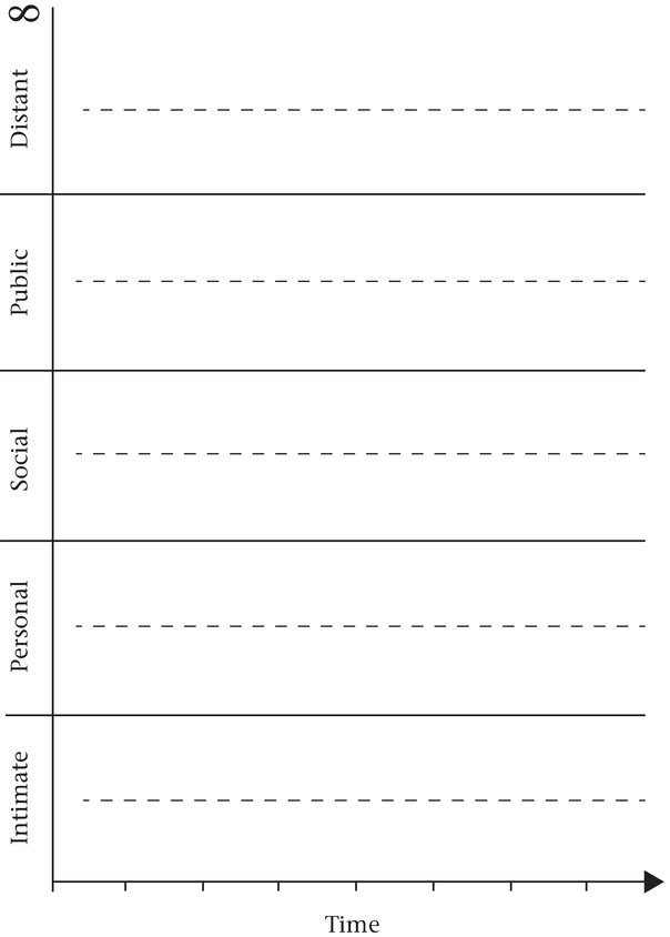
Figure 8.6 Distance location graph, divided into five distance zones, each divided into halves.
The Y axis is divided into the five distance zones. Zone sizes in the graph do not reflect their disparities of physical distance. Zones are of equal size here, to acknowledge equivalence—that all zones hold equal potential to contain sources. All five zones occupy a similar amount of conceptual space, but represent significantly different amounts of physical area.
The size of the zones can be adjusted to most clearly present the positions of sources. Zones with considerable activity are enlarged, and those with no activity are contracted. Public and distant zones may be omitted from the graph entirely when they contain no sources, though the public zone should be present (though perhaps contracted in size) when a sound appears in the distant zone. The intimate zone should be present in all graphs (whether or not it contains a sound) as the empty zone provides the sense of separation from the listener position to the other zones.
In practice, it is not unusual for tracks to locate more (or most) sounds within one zone than in others, and even to exclude some zones. This distribution and grouping of sources within distance zones represents an important spatial characteristic of tracks.
Sound sources are placed on the graph as thin lines, marking a precise location of the source from the listener. Observing the source at a discrete distance from the listener yields the most pertinent and useful impression of distance. These distance positions and relationships of sources generate the substance that will be evaluated and generate conclusions.
Some may find it useful to include information of sound source host environments (spaces) to distance observations. A sound source’s space might be notated as an ‘area’ on the graph, with the source location still visible within that space; the area represents space’s front and rear edges. This process combines observations of environments (that will occur in a following section) with observations of distance location. While this combined observation can be useful in understanding many tracks, the process can be confusing and not readily performed accurately. This combination will often be represented more directly on sound stage diagrams, where they can be shaped without temporal concerns; these diagrams will be discussed in the next section.
The process of collecting observations for distance typically follows the sequence:
- Focus on a specific sound source (or sources) to be observed
- Identify the source's level of timbral detail (content) at its initial appearance in the track
- Locate the sound within the appropriate distance zone by its context
- Compare content and context observations to refine zone decision
- Locate the source at a precise position within that zone
- Position the source relative to other sources, as appropriate
- Repeat this process as the source progresses through the track
Listening attention will shift between several levels of perspective. These observations are at the following perspectives: within the sound source (timbral detail), of the individual sound source (context, locating sources within zones), and at the composite texture (positioning sources relative to one another). Praxis Study 8.4 can assist one in acquiring facility with this important spatial property, and in creating distance location graphs.
Figure 8.7 allows us to observe several distinct distance relationships and shifts in distance positions. Listening for timbral detail, the maracas are closest to the listener position in “A Day in the Life” (1967, 1987). The acoustic guitar is the next closest source, it changes distance at the beginning of the passage, and again during measure 26. John Lennon’s vocal is slightly farther from the listener than the guitar; while the line contains a significant amount of reflected sound, its timbral detail establishes its presence within the listener’s personal zone. The lead vocal is embedded within a small area shared by the bass and the acoustic guitar; they are near to each other yet distinctly separate. The graph does not contain all of the nuance of distance changes that occur within each of these sources; their presence on the graph is somewhat generalized, though representative of their location and general activity. The remaining percussion sounds are omitted; it will be informative to notice how the percussion sounds extend the sound stage depth by their distance positions.
Typology of Distance
Table 8.6 is a general listing of topics that might be collected for distance positions, assembled as a typology table. The table can extract data that has been collected from X-Y distance graphs in various ways depending on the goals of the analysis and the qualities of the track. A typology table will often be defined by the sources it contains and the time space of the observations. It might encompass all sources, or be limited to a specific few; it may observe the content of verses, or of any other section; many other options exist.

Figure 8.7 Distance location graph of the initial sections of the Beatles’ “A Day in the Life” (1967, 1987).
Table 8.6 Typology table of general attributes and values for distance position of source images, and for depth of sound field.
| Variable or Attribute | Values* or Characteristics |
| Positions of Sound Sources | Direct sound, or front edge of distance images |
| Identified for individual sources | |
| Collected for all sources (sound field) | |
| Comparisons: nearest, farthest, most common positions identified by zones, or regions within zones | |
| Groupings of Sound Sources | Sources within identifiable regions of the sound field (bonded by proximity to one another) |
| Sources bonded by appearance within the same distance zone | |
| Movement of Distance Position | Speed of motion (duration sound in motion and distance traveled) |
| Regularity of motion's speed | |
| Beginning and ending positions | |
| Depth of Sound Field | Location of nearest sound source |
| Location of farthest sound source | |
| Amount of area spanned from nearest to farthest sound source | |
| Density of Sound Field | Region(s) of source congregation |
| Position(s) of isolated sound sources | |
| Region(s) void of activity | |
| Amount of space separating sources or groupings of sources | |
| Sound Field Profiles by Structural Division | All source locations during specific structural section(s) |
| Contrasting sections observed as separate profiles | |
| Patterns of alternating profiles (i.e. patterns created by alternating verse and chorus sections) | |
*All values represent a placement of image within specific distance zones; for precise identifications of position, a percentage calculated between the closest position (0%) to the farthest position (100%) within a specific zone's continuum of space can be stipulated.
The listing of attributes and characteristics in the table is by no means comprehensive. Other topics can be added, and its content shifted. Thereby, an analyst may choose to use the table to organize and bring a degree of clarity to other distance information particular to one’s needs. As one example (of potentially many), variations in the lead vocal’s position between structural divisions, perhaps including movements of positions within sections, can be central to some tracks; this data will allow comparing these to the context and delivery of lyrics.
SPATIAL STAGING AND SOURCE IMAGING
Spatial staging can serve as an initial point of departure for discussions of sound source positional placements and relationships. The sound stage represents an illusion of a space of physical size, an area in space defined by width and depth from the point of audition. Sound sources appear as aural images within the hollow space between the furthest possible left and right lateral positions and the nearest intimate and farthest distant locations. ‘Staging’ recognizes the positions and interrelations of sources.
The sound stage encompasses the area within which all phantom sound sources (invisible aural images of instruments and performers) are perceived as being located. It is a two-dimensional area of width (stereo field) and distance (the illusion of depth of field). The sound stage is the area from which all sources of the track emanate, or where they are staged in a single grouping. This concept of ‘staging’ may be a metaphorical or a functional representation of a performance—depending on the track.
‘Sound stage’ is a convenient metaphor, connecting the virtual area within which source images appear to be congregated with the concept of the staged performance, with all sources congregated in ensemble. As such, the term does not imply staged performances are always present in popular music records—or even that they are the norm. The metaphor of staging is helpful in conceptualizing (and ultimately recognizing) the boundaries of the sound stage. When taken a step further, the metaphor establishes the front edge of the sound stage; the relationship of this front edge to the point of audition allows the degree of listener connectedness to the track to be observed.
The sound stage does not impose a fixed model for understanding positions of recorded sounds; nor does it impose a fixed area within which sources may emanate (except, of course, those imposed by principles of acoustics). Rather, it is an open void within which sounds of the track appear; it is a hollow space where sources are positioned without predisposition other than conventions of the track’s style. The sound stage provides a platform where the positions of sources can be observed, and the spatial uniqueness of the track recognized.
In ‘Listen to My Voice’ Serge Lacasse (2000a) has offered an extensive study of vocal staging, engaging many significant matters of the voice in recorded popular music; while his study has its focus on the single vocalist, it can help us focus some broad issues engaged here. He provides a useful distinction of process and object: “in that ‘vocal staging’ refers to the practice taken as a whole on an abstract level, while ‘vocal setting’ refers to a specific ‘embodiment’ of the (general) practice of staging” (Lacasse 2000a, 5). In applying these definitions to applications of sound stage, the term ‘staging’ is here defined as the process of establishing or observing the sound stage; it is the overall act and conception of recognizing stage dimensions and attributes in the abstract. The term ‘setting’ is a bit problematic here; the sound stage is at a higher level of perspective (see Table 8.1) and more complex than the setting of a single source.
The term ‘scene’ would be more appropriate for an individual sound stage diagram, representing that which results from the act of staging—the ‘embodiment’ of the sound stage content. ‘Scene’ brings to mind a portion of a dramatic work, a section unified by some identifiable context, and that exists within a specific period of time within a larger whole comprised of additional scenes. Further, there is also a connection between the sound stage and ‘auditory scene analysis’ (Bregman 1990). Auditory scene analysis is a psychoacoustic phenomenon that involves dividing up the components of a complex wave (a complicated auditory experience) into auditory objects on the basis of grouping cues; groupings may be based on spatial location, spectral content, time or onset. The individual sound stage might be considered a ‘scene,’ as a complex auditory image based on spatial groupings of successive and simultaneous sound sources. Considering each sound stage as representing a span of time allows it to coalesce into a singular complex auditory image or scene; this image or scene contains the arrangement of the positioning of all sources as a single group (sources may be either stable or exhibit change). The notion of ‘auditory scene’ provides a useful way to consider the particular arrangement of the myriad of qualities within an individual sound stage (Schnupp, et al., 2012 223–267).
Track as Performance
The track is its own performance (A.F. Moore 2010, 264). No matter if its performance appears to happen like a live event, or if the performance is utterly impossible to have occurred given human and worldly limits, the sounds of the track unfold in time and are linked to the origins and expressions of its sounds. Zak (2001, 43) frames this matter: “[R]ecord making represents “out loud” musical thinking. Ideas are not merely expressed in sound; rather, ideas become sound. Thus, concept and performance enter into an integral relationship that we perceive as a whole.”
The track is “a schematic representation of some real or constructed performance” (Zagorski-Thomas 2014, 6); a performance that is directly experienced, often deeply and viscerally. We hear it, feel it, react to it, sense its physical gestures, interpret the effort and expression of the performances. Further, we seek to identify the location where the performance is happening, our physical relationship to it, and so forth. There is a natural human need (a survival trait with inherent skill, that is more visual than aural) to identify where sources are located—and attend to them accordingly. Spatial staging provides the analyst (or listener) access to observing the positioning of performers and the performance.
Our “natural tendency to relate sounds to supposed sources and causes, and to relate sounds to each other because they appear to have shared or associated origins” (Smalley 1997, 110) is an important part of experiencing the performance; the performer is source-bonded to the instrument (or voice) which generated its sound. Sound sources are bonded with our sense of their origins—a human or technological player, generic or specific instruments/voices, timbres, aesthetic materials, and also spatial environments and spatial identities. The sounds of sources evoke the presence of their performers, and the gestures and interactions of performances. The spatial positioning of the virtual performers adds dimension and richness to the experience, as sources bond by association or sharing perceived origin or cause.
Spatial staging locates the track’s performance and its sounds—and all that they carry. It provides a sense of where the performing ensemble is, in relation to the listener. The sound stage not only localizes the ensemble, but places each sound source (its aesthetic materials and sound qualities, its instrument and performer) in space. Sources are in a place; they are at angles from the listener’s center, and at a distance from their point of audition. And, sources can move. Zagorski-Thomas (2010, 252) relates the staging of tracks to those of staging a play:
Earliest stereo recordings placed sounds in relationships that performers typically formed on stage. This was a rather simple matter for orchestral and choral recordings, with but a few choices of locating sections (King 2017); jazz groups could get a bit more complex, but not significantly. For popular music performances, a group’s live stage layout is often casual and varied between performances; staged positions of players are quite arbitrary, not rigidly established. On stage, drums might be more or less centered, with instruments to either side, and vocalist front and center, though even this loose connection is meaningless to the sound and performance, except for performer interaction. Amplification and mixing the sounds of all instruments and voices determines the perceived positions of sources; the stage locations of performers is not reflected in what is heard through sound reinforcement systems. In the track, convention established—for technical reasons of LP record grooves as much as musical—the perspective of a listener facing the bandstand; vocalist at center stage, drums behind (kick drum centered, snare drums centered or slightly left, high hat perhaps about 10º to the right, toms and cymbals balanced left to right), bass centered, other instruments spread out to balance the stereo field and to be clearly distinguished (or blended). It did not take long for these positional relationships of rock performers on records to break their connection with a virtual stage. While some tracks retained a connection to the stage, others used spatial positioning of sources as variables to shape the track. Staging was used to create unique spatial relationships between aesthetic ideas and the sources (performers and instruments) that produced them. As early as 1966, with the Beatles’ “Tomorrow Never Knows” we witness a dramatic shift away from common staged relationships; the track fully embraces an aesthetic that instruments and voices (and source-bonded representations of the lads that played them) are untethered by the laws of physics. The positioning, motion and environments of the sources on the sound stage also shaped the character of the track, both from drawing listener attention and from being absorbed into the track’s texture.
Popular music recordings treat space as an aesthetic canvas. Locations of sources may be at any location (lateral, distance or room) an artist believes best suited to their expression and aesthetic. Spatial properties blend into the essence of sounds and materials, become part of their character and content. Much artistry is involved in inventing worlds where sounds have unique or surreal spatial qualities, relationships that defy physics. “The more unique the space is, the less it represents experiences of sound in the natural world and the more the record takes on the quality of a dramatic stage” (Zak 2001, 145).
Staging and Listener Interpretation
The concept of a sound stage may be predicated on the listener conceptualizing the track as a staged performance, one occurring in front of them (Moylan 1992, 2012, 2015). While this may not hold between individuals—or especially between cultural segments—it is one tangible way to conceptualize, organize and interpret sound location. The concept of a performance in front of the listener, within some virtual place, is not a stretch; in fact, it is a common perception to those with considerable exposure to staged performances. Staged performances (on stages humble and grand, from concert halls to pubs, churches to amphitheaters) are cultural norms to a great many listeners. With personalized listening experiences, “listeners often conceptualize acousmatic sound by comparing it to previous experiences with sound” (Brøvig-Hanssen & Danielsen 2017, 194); listeners are prone to interpret the staging of the track as an association to some listening event of the past. Whether tracks are ‘heard’ as emanating from a stage or as staged in some other manner is a matter of listener interpretation.
Production shapes the spatial qualities of the track—and the listener interprets them. Recent production practice for popular musics has not aligned spatially with concert listening. It is rarely relevant to carry expectations of concert listening spatial properties and relationships into an analysis. Individuals have internal spatial references, shaped by past experiences of live music listening in various venues and by listening to certain production styles (Brøvig-Hanssen & Danielsen, 2013).
The contexts of live performance vary by culture, and by styles of music; formal staged performances will be foreign to some, common to others. While some listeners—for example those who regularly hear classic rock records—might recognize relationships of performers that might realistically be staged in performance, others’ perceptions might transport them to the corner of a local pub, others to a street scene, etc. Dance music, and other genres (those existing and those yet to be devised) may well be heard differently.
Some tracks cannot be (or will not be) interpreted as staged performances. The materials, character and content of sound sources can bring spatial positioning of performers (sound sources) within the track that have no relation to prior live listening experiences. A ‘performance’ may not emerge from the track at all for some listeners; further, the track may not be presented as a ‘performance’ by an artist. This is among the aesthetic statements of the track, and amidst the factors interpreted by listeners. For example, it is unlikely numerous listeners would imagine a staging of Peter Gabriel’s “Intruder” (1980) as a humanly possible, live performance taking place in front of them. If the listener conceives “Intruder” as a gestural performance at all, it might tend toward the cinematic, or perhaps some other, more personal manifestation.
The listener may locate their point of audition at center stage, sound coming from a performance in front of them—though perhaps not. Even the point of audition can be a variable for some listeners, along with the acoustic variables of automobile seating and ear buds, there are conceptual matters where some listeners are prone to projecting or placing themselves within the contexts and activities of songs. Listeners will have diverse experiences, and will bring diverse backgrounds and expectations.
A sound stage cannot represent a singular cultural experience—contexts are not universal among many listeners, and many diverse cultures are represented within the expanse of popular music genres. Popular music is mostly experienced as records, not in live performance. When popular music is experienced (performed live), sound reinforcement systems very typically render the physical locations of performers meaningless, as their sounds are blended and presented to the audience through the same loudspeakers. In the end, listener interpretation of the ‘performance’ cannot be anticipated; the listener’s conception of the sound stage may be highly personal at some level, and hold cultural norms in other ways. The notion of a sound ‘stage’ may simply be a location for the ‘staging’ of sounds—the notion of an area in which the sources are congregated.
Sound Stage and Analysis
Based on the previous discussion, the concept of sound stage may be defined to serve the analyst’s purposes and conceptions. The concept is sufficiently malleable to allow the record’s representation of spatial properties to be organized in a way meaningful to the listener or the analyst—and pertinent to the unique attributes of the track. For the analyst, the sound stage provides a reference; it can aid in explaining the track’s experience of spatial positioning of sources to others, as it provides a conceptual common ground based on the analyst’s perception of the spatial properties produced by their playback system.
This approach to sound stage as a conceptual common ground, can allow positioning of sources and the size of the overall area they occupy to be identified and observed. The dimensions of the sound stage and its content can transfer to the listening experiences of others, and provide common points of reference. While some variation will appear between playback systems, a basis for common experience (of some significant substance) of the sound stage will emerge. As a single space, its size is defined by its boundaries left to right, front to back; it can be precisely calculated in degrees left and right, and by nearest and farthest placements in percentage of specific distance zones.
The listener groups all sources to occupy a single area—an area from which the track is staged, and its ‘performance’ is heard. Even sound sources occupying significantly different locations within the sound stage may bond and group into the illusion of a single ensemble; an aesthetic alternative, sources may be caused to segregate into subgroups, or some individual sources appearing isolated. For example, it is common for the lead singer to be detached from the group of the accompanying instruments—the textures established by the functions and relationships between the lead vocal and accompaniment take many forms, and may at times segregate into separate streams. Other permutations are possible as the individual track asserts its own aesthetic—for example, lead singer separated from background voices, separated from accompanying instruments. Still, some rock styles position the singer very close to the instruments, as if with the band.
Sound Stage Diagrams: Notating Image Positions
An early writing on the sound stage articulated its relationship to the performance: “. . . a two-dimensional area (horizontal plane and distance), where the performance is occurring . . . The sound stage is the location . . . where the sound sources are perceived to be collectively located as a single ensemble” (Moylan 1992, 207–208). The dynamic nature of some sound stages in rock music could not be reflected in a single sound stage diagram; these diagrams were intended to synthesize observations from stereo and distance graphs. Early approaches to charting stereo location and distance placement of sounds made clear the need to engage sounds in surreal positions and relationships (Moylan 1986). Spatial staging became a way to account for perceived locations of sources found within tracks, whether or not they conform to real life experiences; it allowed for the collective location of the ensemble to be conceived in relation to the overall environment of the track and to the listener position. In this way, the sound stage could be used for production planning; as an analytical tool it could also be used for evaluating the aesthetic of the track in relation to its simulation of real-life experience(s) or representing the surreal (Moylan 1992, 79–89).
The sound stage can function as an analysis tool (Moylan 2012, 180). In illustrating the locations of sources, the following sound stage variables might become visible:
- boundaries of area containing all source placements
- densities of sound source distribution throughout the sound stage area
- the relationship of the collected sources to the listener
- the relationship of sound stage and the holistic environment
In the physical world, lateral cues and proximity discrimination work together for positional localization. This two-dimensionality is transferred into the record. Sound stage diagrams reflect these real life percepts and interrelationships; the physical objects that are heard and localized with the significant assistance of sight in everyday experiences are represented as phantom, aural images in the track. The placement of aural images on the sound stage establishes an illusion of positional relationships between sources and between sources and the listener; “[T]he apparent location in space of sound sources, near or far, left or right, does refer to the simulation of actual spatial dispositions” (Doyle 2005, 27). It may be obvious, but is easily overlooked, these relationships also extend to encompass the musical materials presented by the sound sources, as well as the location of the narrative and persona of the lyrics.
Staging diagrams do not include non-spatial elements. They are dedicated to the two spatial properties, and are capable of significant detail and accuracy. Other elements, such as the frequency registers of timbral balance may be compared to spatial staging at later steps in the analysis process;15 this will be covered in Chapter 9. The sound stage is intentionally limited to representing two-dimensional space in order to provide focus on those percepts and to make possible a high degree of detail and precision in observations. Staging brings the percepts and observations of stereo location and distance positioning into a single two-dimensional perspective.
Two sound stage formats can be of use for different purposes: (1) proximate sound stage and (2) scaled sound stage.
The (1) proximate sound stage is visually uncomplicated; it is an empty staging area, with loudspeakers placed as a reference for angle only. This sound stage format is useful for showing approximate (or generalized) sound source placements and their size; it can be refined to be fairly accurate, and to locate images very near their actual positions. The (2) scaled sound stage format is capable of illustrating precise locations—it incorporates a grid of increments specifying degrees left and right from center and distance zones (adapted in size to suit the example), scaled for precise placement of images.
Importantly, all staging diagrams are snapshots of time; they represent a specific time period (with a beginning and an end point) or a specific moment in time. The time period might be any suitable length: a phrase, a song section, or in some cases, the diagram might represent the entire track. The longer the time period, the more generalized the observations. Moving sources are difficult to notate on the diagrams, as there is no temporal axis. The X-Y graphs for lateral and distance location can clearly notate any source exhibiting motion.
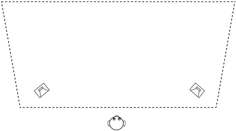
Figure 8.8 Proximate sound stage, for generalized image placements.
The proximate sound stage for general positioning of sources is valuable for sketching initial observations of source positions. This format does not position the listener and the loudspeakers in an equilateral angle, but rather allows a conceptual placement of sources in relation to relative positions of loudspeakers and the listener. Placements have the potential to be more or less precise in relation to the loudspeakers, and the listener, as determined by the analyst (their needs and abilities); the diagram does not contain the divisions necessary for exact placements. Instead the diagram serves two functions that might be important to analysis.
First, the proximate diagram is useful for sketching image locations during initial listening sessions. One’s first impressions of stereo imaging and distance locations can be noted, and developed upon repeated hearings. The analyst can obtain a sense of the positioning of sources and the extent to which more detailed analysis might yield significant information. Listener position and distance zones can be sketched along with the aural images; the analyst can adjust the diagram to best suit the analysis and the material being observed. From these sketches one is able to obtain a sense of the important attributes and levels of activities within the track’s sound stage; and the need for further detail in the observations. One can decide an appropriate course for the analysis from the available options to:
- Create an X-Y stereo location graph to explore locations in detail, with a sense of temporal progression of the track, or of sources that change widths or locations; this may be for all or for select sources
- Create an X-Y distance location graph to explore locations in detail, with a sense of temporal progression of the track, or of sources that change locations; this may be for ail or for select sources
- Refine a proximate sound stage diagram for all or for select sources
- Establish a scaled sound stage diagram for all or for select sources (perhaps with the remainders on a separate general sound stage diagram)
Second, the proximate sound stage diagram can provide proportional and relational placements of sources with enough detail to be useful in many contexts. This generalized diagram may often be all that is needed to notate the positions of sources, and to adequately observe these properties in sections of the track.
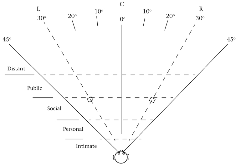
Figure 8.9 Scaled sound stage diagram for precise localization of images.
A scaled version of the sound stage diagram locates the listener and loudspeakers in an equilateral triangle relationship, and with a sense of distance zones. This scaled sound stage is capable of illustrating precise locations of stereo placement, and the listener’s considered interpretation of distance placement within specific zones. This data can be sketched first on a proximate graph, and refined in final form here. Perhaps most directly, the scaled staging diagrams can organize and reframe data collected in stereo and distance X-Y graphs; those graphs bring focused attention to the percepts and their placements, and are directly transferable to these diagrams.
Figure 8.9 illustrates the increments of degrees for lateral positioning of sources and distance zones; these are scaled for precise placement of images. The area for image localization projects from the point of audition, in a 90º cone that stretches to the horizon of the sound stage. The positioning of the loudspeakers pertains to lateral imaging only; extra reference lines guide image calculation and positioning.
The visible loudspeaker placements on the diagram are not relative to the distance zones, and are irrelevant to distance positioning; they are included to assist placing sounds in the stereo field and should be ignored in establishing distance locations of sources. It will be helpful to identify distance of the source by timbral detail (perhaps placing the sound on a general diagram or a distance X-Y graph), and then proceeding to determine the position and width of the image at that distance position on the sound stage. Distance zones incorporated into the scaled sound stage may be size-adjusted to most accurately or clearly illustrate the track being examined. The subjectivity inherent to some distance calculation can be noted and minimized by describing one’s observations and processes of deduction during analysis discussions.
The point of audition perspective of the track will often bring closer images to be wider sources; this is clearly evident in this approach to staging. Here again this approach brings sound stage imaging to mirror our perception of how lateral images appear to change size (occupy more of our perceptual field) as they move closer and farther from our point of audition.
Typology of Staging
Typology tables will assist in organizing the many variables of the sound stage, and can reveal their characteristics and interrelationships. The typology table can also make clear the way the sound stage functions on all three levels of perspective.
Functioning at the overall perspective, the sound stage establishes a sense of physical boundaries for the track. The dimensions of the sound stage and its containment area establish important contextual attributes of the track’s spatial identity. These can be clearly identified or defined in the typology table.
These sound stage dimensions and attributes characterize sections of the track; with movement from one section to another staging changes are common. The characteristics of the verse sound stage typically return with the verses, perhaps with some modification; choruses, bridges and middle eights typically have a contrasting overall size of the sound stage, and internal attributes. Progressing between sections of the track can be accompanied by a sense of movement from one ‘auditory scene’ (Rumsey 2001, 43–44) or set of spatial relationships to another. Separate sections of the track are most readily observed and evaluated using individual typology tables, and individual sound stage diagrams, for various sections of the track (as appropriate).
Table 8.7 Typology table of proximate and scaled sound stage attributes and values.

Because stereo (lateral) localization and distance location are part of the sound stage, their typological concerns (just discussed) are imbedded into those of the sound stage. The perspectives of activities of individual sound sources and of composite texture come together in these localizations. Individual sources reveal their positions and widths or depths in the sound stage’s two dimensions; this positioning and size information is then available for comparisons at the composite texture’s perspective. Sources can be compared to one another; from this process, patterns and groupings of locations and attributes might be recognized, areas of density and voids within the stage become apparent. The stage can be fluid or fixed; source locations in flux or those that are unchanging mark the extremes within which much gradation can occur. The left-right and front-back boundaries and the dimensionality of the sound stage have the potential to change, just as each source has the potential to change; the sound stage as the overall space that contains all of the sources may change, and in so doing shapes the character of the track (by what its size and other attributes mean to the listener) and its sonic content.
For example, the great spatial complexities of the sound stage of Kate Bush’s “Get Out of My House” (1982) combine lateral image locations and sizes, distance positions and depths, and attributes of sound source environments into a complex spatial tapestry of great and continual flux. Studying such a sound stage thoroughly is facilitated by examining all of these elements in significant detail; this cannot be accomplished by any single set of data. In contrast, the sound stages of numerous tracks depict scenes that unfold, often moving alternately between positions for choruses, and continuing to return to a place of the verse’s story, and a similar sonic quality of relationships of sounds; the result is a sense of stability within a changing landscape. Examples of tracks that alternate scenes are many; the primary variables are the types of changes of source positions (lateral or distance) and the amount of change. For instance, “Something” (1969) by the Beatles is typical in that the chorus retains several distinguishing features from the verse while adding several new spatial qualities and shifting the distance position and lateral size of the lead vocal; Adele’s “Hello” (2015) transports the listener to a very different world between the verse and chorus—and a very different character of the sound stage and the track.
Notating the significant activity (on one extreme) and the stable spatial context (on the other) of the sound stage can present challenges. X-Y graphs are able to clearly illustrate these activities and changes for either stereo location or distance positions as they change over time, but comparing the two dimensions is difficult with these graphs. Using these graphs in tandem with sound stage diagrams may best illustrate these essential qualities of many tracks; the diagrams allow the numerous qualities to be visualized, and the X-Y graphs allow for details of size, position and movement. Distance and lateral positioning of sources and size of their collective area are not the only spatial dimensions, though.
The aural image holds the spatial identity of the sound source. This is more than its width and lateral placement plus its distance from the listener and depth. The characteristics of sources’ host environments contribute additional depth cues to aural images, and may also provide added width. Images appear in virtual space with qualities of direction and distance from the point of audition; they also contain breadth and depth from their individual environment’s cues (including those generated by reverb and discrete reflections). The spatial identity of each source is an amalgam of these three attributes, or spatial properties. These will be explored in the following section.
A kaleidoscope of spatial activity can churn within the sound stage—activity that is not only of spatial properties, as the sound stage is the platform on which the sources and all of their activities and qualities are heard and interpreted. The sound stage is the venue for the track’s mix. Within it music elements and lyrics fuse with the spatial qualities; placement of aesthetic ideas in space and their relationships to the listener and the overall sound stage can be observed and evaluated. We will return to staging in Chapter 9 within the mix. At that time additional elements, such as timbral balance, will be observed simultaneously with spatial positioning—other approaches to examining positional, environmental and frequency spaces of the track will also be introduced there.
Peter Doyle offers the following words. They are a pertinent way to transition from positional staging to the spaces within which sounds emanate—and point to the significance of each in communicating the track’s message.
Discussed next, the holistic environment (which might also be considered the host environment of the sound stage) coupled with the attributes of the sound stage establishes the spatial identity of the track.
THE SOUND OF PLACE
In nature, the space in which an event occurs has a sonic quality, a sonic character—indoor spaces and spaces in the open air. From caves to cathedrals, closets to concert halls, all places produce a sonic sense of their proportions and the materials of their surfaces. Places have a sonic presence. Instruments, voices and ensembles acquire sound qualities from the spaces in which they perform. In much of our daily activity, this ‘presence’ is a backdrop for our life experiences in the physical world. The places (spaces and physical environments) of our life events have sonic character that provide context for our activities and experiences. Within all discussions of space, the term ‘environment’ will be defined as the perceived or virtual space within which a sound source seems to be sounding (emanating or performing); an ‘environment’ can be any enclosed space or the open air.
Sounds excite the acoustic attributes of spaces from the actions of their sound waves; sounds are bonded with the spaces within which they were produced. We expect sounds to emanate from within spaces—to be linked with the physical world. In records the perceptions of sound sources are wed with a sense of the space from which they are perceived to emanate; a source is perceived as fused with the space within which it is performing—the fusion is both sonic and conceptual. “The idea of source-bonded space is never entirely absent” (Smalley 2007, 38). “Sounds . . . carry their space with them—they are space-bearers” (ibid.). The sound of a space is bonded to the track’s instruments, voices, performers, performances, materials, etc. Bonded to the source, too, is all that the space represents culturally and to the listener, and its cultural meaning (Doyle 2005). This blended sound informs us of the space of the source, and the connotations carried by the space; the sonic environment of a cathedral might conjure some sense within a listener, or metaphorically represent it within a track.
We know the sounds of spaces; we remember the sound of a place. The listener remembers or ‘knows’ the sounds of spaces, as overall qualities comprised of many factors that are mostly perceived unconsciously, similar to timbres; this perception and prior experiences are used to recognize and understand the spaces encountered in records. “When people engage with acousmatic musical sound, which has no visible source, their experiences with these sorts of different acoustical reflection patterns allow them to imagine specific actual spaces” (Brøvig-Hanssen and Danielsen 2017, 197); reflection patterns and other attributes of environments that characterize spaces are recognizable.
In records, the sound attributes of spaces become part of each sound source (‘host environments’), becomes a dimension of the overall quality of the track (‘holistic environment’), and becomes integral to the track’s content and expression. Each sound source will appear within a ‘host environment’; these environments may be unique for each sound or shared with one or more other sources—each instrument and voice in a track has the potential to be in a different space. These ‘host environments’ are situated at the basic-level of the sound source. The bonded sound sources plus their host environments are localized on the sound stage, where all sources within the track form a singular grouping (that is the ‘performance’ of the track). The ‘holistic environment’ is the space of the sound stage—the place where the track is perceived as existing. All instruments and their spaces are amalgamated into a shared space, and a holistic character forms, if not a recognizable space. The holistic environment is resident in the large dimension level, and is a dimension of the overall sound. Thus, a hierarchy of space exists, where spaces can be imbedded within other spaces—spaces of sources are housed within the overall space that contains the sound stage.
It may now be getting clear, tracks present environments in unnatural ways; they change space and our relationships to spaces. They bring us spatial variables and attributes that are well outside our worldly experiences.
The spaces within tracks might be polarized ranging from natural spaces (captured while the sources are recorded), to fully fabricated, with their attributes crafted and invented—though most fall somewhere between. Such invented virtual spaces are often sonically and experientially unnatural, having qualities that nature cannot generate. Physics and acoustics are no longer limitations; sounds of environments in records are created technologically (from many options, each with its own sonic imprint), captured (within the recording process) or manipulated (through various mixing and processing techniques); their attributes need not align with the real-world. The listener accepts unreal or surreal qualities as being suitable places for sounds and tracks with little hesitation—we seem willing to readily accept as plausible a physical environment that is not of this earth, that was fabricated to support the qualities of the sound source, and that is integral to their experience of the track. Brøvig-Hanssen and Danielsen (2016, 27) observe: “[M]usical spatiality has a tendency to point the listener toward a real-world physical phenomenon even as it acts to undermine that reality.” We might recognize a continuum, of sorts, spanning from two extremes. On one end are real sounding spaces; environments that embody sonic attributes of the natural world (and that listeners may have actually experienced). On the other extreme are those that are utterly liberated from physics—void of Earthly sonic attributes. Environments may take a myriad of forms stemming from how they are established, the values of their attributes, and their relationship to known spaces.
Even those environments that are ‘natural sounding’ hold traces of technology, however; a microphone imparts some degree of its unique, inherent sound quality onto the space that is recorded along with the source (Moylan 2015, 360–363). “Any sound recorded by a microphone bears some degree of patina imparted by the space in which the sound was produced” (Zak 2010, 313). All recorded sounds bear the sound of the place of origin; even the subtlest of room sound situates a sound in space. All sounds come from places, whether natural spaces or created environments; within the track all environments are to one extent or another simulated spaces, holding the imprints of the technologies that captured it. It is natural for the listener to perceive the source within a space, no matter the source’s spatial content. When sounds display no noticeable environment attributes, “the most likely interpretation . . . would be to hear the voice as sharing, or as sounding inside, the listener’s own environment” (Lacasse 2000a, 193).
As this section unfolds, we will engage the content of environments and their character; this linkage with timbre is intentional, and will become clear. Discussion of physical content of spatial environments, and of echo and reverberation, will allow observation of the subtle qualities of spaces, and of their appearance in tracks. Such appearances give opportunity to engage the character of spaces. Spatial environments organize into hierarchy; bonding of sources with their environments, the rich potential of relationships of spaces, and the holistic environment bring potential new richness to spatial character. Entwined in the microscopic details within the attributes of environments, is the deep listening required to hear their values; this is another connection to timbre—this time for analyzing and recognizing portions within sounds that we previously ignored, as they coalesced into the whole.
Sound Source Host Environments
All sound sources in the track emanate from a conceptual performance space, or environment. This space is a ‘host environment’ for the sound source; it ‘hosts’ or contains the sound source and the sounds it produces. In real life, sound sources will most often share a host environment with other sources—we talk amongst friends in the same room, sounds are around us on the street, performers share the same stage, etc. Often in tracks, though, individual sound sources are situated within their own space, contained in a separate room or environment.
The many sound sources in tracks may each be located within a different host environment; each source may be bonded to and hosted within a uniquely different space. Sources may share environments in the track, with several sounds appearing to emanate from within the same space, though perhaps at different locations within the space. Further, it is common for sources to change spaces as a track progresses, and/or for them to change distance locations within their host environment(s). When this happens, it is typically between structural sections, such as between verse and chorus.
The source ‘host environment’ is situated at the basic-level of the individual sound source. As such, it provides the same tangible point of reference of activities of individual sources that we have observed for positional locations of sources.
The attributes of the host environment become part of the ‘sound’ of the instrument/voice; the two fuse into a single percept. They are entwined, as the sound of a space draws out the qualities of an instrument or voice within it, just as a sound source excites the qualities of its host environment. Environment qualities contribute to and shape the sound’s content and character, and add other dimensionality to its spatial identity. The host environment also reinforces the source’s performance, situates the source and performance in a physical setting, and can influence stream segregation’s delineation or blending of sources and the materials. Host environments, and their environmental characteristics, have equal potential to shape the track, along with all other elements.
In surround sound, the environment can appear disassociated from the sound source (direct sound), appearing as a source in itself. Mirroring the original sound to some degree, such an environment is separated spatially from the source, in a clearly different position. The tendency of the source to bond with its space makes this segregation very difficult to accomplish in stereo. This separation is often found in surround sound, though, and it can take many forms (Moylan 2017, 44–49). For instance, in surround sound sources may often be located in front of the listener with their host environments behind, providing some dispersion qualities similar to the way the sound of live performers might fill a space (the LOVE version of “Strawberry Fields Forever” is an example of this separation); localization of sources (in lateral location and size and distance positioning and depth) and their host environments (either bonded or separated) is complicated in surround and carries distinct differences from stereo (see Moylan 2012, 2015, 2017).
The hi-hat sound in two contrasting versions of “Let It Be” allows us to recognize the unique qualities of their host environments; as they are rather isolated in the second verse (beginning at 0:52), this contrast is starkly apparent. Diffusion is important to the host environment of the source in both versions. Diffusion of a reverb is the lateral dispersion of the reflections and reverberation (in playback) and the density of those reflections.
George Martin’s version, remastered for the 1 (2000) release, provides the hi-hat with a host environment with sparse reverberation diffused over a significant area. The reverberant sound is quite uniform in the amplitude of its reflections and is only subtly different in spectrum from the direct sound. The pre-delay is very short (in the range of 3–4 ms) with the reverberation established quickly; the content of the host environment does not mask or disguise the subsequent attacks of the hi-hat. This host environment provides some significant sonic interest, as the instrument’s reverberation disperses to one side of the sound stage away from where the attack of the sound occurred. The hi-hat is located in the area between 17–25° right of center. After the attack, the reverberation disperses to the left, ending at 25° left of center; it takes place in less than a half-beat for the sound’s reverb to travel across the sound stage, and the reverb tail is a bit less than the duration of one beat. The reverberation is increasingly sparse as it spreads across the sound stage; there is an impression that something causes the reverberation to stop at that point in space, perhaps interpreted as a reflective wall on the left that is the source of the subtle echo that is established as the reverberation stops spreading.
The host environment of Phil Spector’s hi-hat has width of approximately 19°, extending from 7° left of center to about 12° right. The direct sound of the hi-hat image occupies the space from 3° left of center to 3° right; this direct sound width is confirmed by the closed hi-hat strikes in the chorus. The sound pulsates within that environment and the echo iterations spread the image around the direct sound to fill the area. The pronounced tape echo on Ringo’s hi-hat generates a prominent 16th note pre-delay that provides the impression of a large space with highly reflective surfaces (and that also reinforces the rhythm of the music); the echoes continue at the 16th note (with subtle 32nd note echoes appearing over time) as the length of the string of echoes coalesces into an aural image of reverberation. As with Martin’s, this host environment has a different reverberation density in various positions. A large cavernous space is implied by all these reflections, and the high frequency area is attenuated as the iterations progress and the low and low-mid range frequency area gradually builds in amplitude, supporting a sense of distant reflective surfaces. As the verse progresses, the attacks of the hi-hat begin to blend into the host environment’s reverberation, the instrument begins to mask itself (reminiscent of Spector’s wall of sound techniques). Spector’s host environment is comprised of rhythmic echoes that become reverberant and become perceived as reverberation; this is explored in detail within the next section.
The host environments of both versions provide the hi-hat with a sense of space and place, and also an impression that an area is spanned with a changing density and varying timbral content. Spector's environment has more unusual and pronounced qualities; Martin’s space is surreal in other ways, though, with its sparse density and motion of dispersion. The character of both spaces has some commonality in their sizeable spaces (though Spector’s is slightly larger) and sense of motion. Here we can witness the host environment contributing to, and supporting, the track’s sentiment and lyric content—though the sound source it contains is presenting a simple back beat.
Echo and Reverberation
Echo and reverberation are reflected sound; each can manifest in various forms. Most of their forms carry a content relationship and/or association with a host environment, though some of their appearances are independent. While they may be conceived as incomplete forms of environments, echo and reverb are acoustic properties of their own. Echo is the result of an extended early time field;16 it results when a sound is distinctly reproduced as it bounces off some distant surface. The time between direct sound and reflections is sufficient for the reflection(s) to be heard as a copy of the original; echo may appear as a single repetition or can multiply, depending on how many times a sound bounces. In contrast, reverberation occurs when the sound is reflected so many times, and in very close time successions, that all reflections fuse into a single sonic impression. As echoes’ discrete reflections move closer in time (time intervals smaller than 100 ms) they cease to be perceived as separate sounds; as this time interval shortens, discrete reflections ultimately blend into a diffuse sound, what we experience as reverberation (or reverb). As such, “echo is perceived as the repetition of an original sound event, while reverberation is perceived as a prolongation of that sound event” (Lacasse 2000b).
The use of these spatial techniques in records began by recording and manipulating acoustic rooms and chambers. Artificial reverberation techniques were soon developed to generate the many reflections—by passing the sound through springs and through metal plates—and ultimately to also control the dynamics, reflection speed and density, and the spectrum of the reverb. Reverberation is an integral attribute of environments; reverb alone (as it commonly appears in tracks) is without the early time field reflections found in real-life spaces. Echo was created artificially through various tape delay techniques, until the digital delays of the early 1980s allowed regenerating sounds to create any echo delay.
Echoes occur naturally in certain real-world environments, as repetitions of sound are generated as the original is reflected. Echoes are generated within very large spaces, containing walls, ceilings, floors and other objects or boundaries of hard surfaces, located at considerable distances apart and from the listener.17 They can also be produced in open air, with sound reflected off distant surfaces and objects before returning to the source location as a repetition or a partial repetition of the original. While in records echoes can appear with qualities nature could never produce, echoes all evoke a sense of extraordinary space. R. Murray Schafer (1977, 218) notes: “[E]cho suggests a still deeper mystery . . . every reflection implies a doubling of the sound by its own ghost, hidden on the other side of the reflecting surface.” Echoes can elicit images, interpretations, meanings and representations of many sorts from within its unique timbral and time qualities.
Further, echoes, and especially a string of echoes, can establish the illusion of a peculiar environment. Echo can provide the experience of extraordinarily large spaces, the outdoors, etc. At shorter durations, a single or small number of echoes represents an incomplete space; certain qualities of real, enclosed spaces are missing. This is neither an issue for the listener nor for the track, it is an assessment of the potential content of reiterated sound. The variables of echoes are the time difference between the original sound and its repetition(s), dynamic relationship between the original sound and each repetition, number of repetitions, dynamic shape of repetitions, and more. Reiterated sounds of echoes may be altered in frequency content, given dynamic shape, and other characteristics to provide greater alignment with the attributes of real-life spaces.
Echoes may appear in other forms, notably (1) echoes bonded to a single source (as in the above hi-hat example from “Let It Be”) and (2) as a separate source. As connected to the original sound, it is bonded with and refers back to its source. The sound source is reiterated, fully or partially. ADT (artificial double tracking) is an example of the echo bonded with its source for timbral effects as well as spaciousness; “I’m Only Sleeping,” “Eleanor Rigby” and other tracks off Revolver (1967) are clear examples of the Beatles’ first uses of this technique. Bonded with the source, echo is used as an effect in many ways, such as the tape echoes appearing at the end refrains within the Beatles’ “Paperback Writer” (1966). As echoes are temporal, they can become part of the rhythmic fabric of the track, bridging the recording and music domains. Echoes can be tuned precisely by recordists, to integrate with the track’s rhythmic elements, or those of sources. Echo is used as part of the musical and rhythmic textures in countless records of the 1980s; two differing examples are David Bowie’s “Let’s Dance” (1983) and “Don’t Come Around Here No More” (1985) by Tom Petty.
An echo may be a separate entity, representing a second sound source that is a duplicate of the original but “separated from the sound in space and time,” with “a presence of its own” (Zak 2001, 77). It is often a single echo. An organ chord inside the left speaker location and its echo inside the right speaker location can be heard distinctly in the introduction through first verse of Bob Dylan’s “Love Sick” (1997); the echo ceases as the texture thickens, and the organ retains its original position without the motion of echo. Elvis Presley’s “Blue Moon” (1954) provides another example, as “the voice’s echo casts a languid shadow clearly audible in the spaces between phrases. Here, the echo takes on a ghostly character that, again, enhances the track’s overall stylistic effect as it reflects the dreamy character of Presley’s performance” (Zak 2010, 317). An echo’s form will have some defining quality that distinguishes it from the source—perhaps timbre, or position, or some other characteristic.
Reverberation is one of the potential attributes of natural environments. It is comprised of innumerable reiterations of the original sound. Among its variables are: duration of the reverb, time density created by the spacing of reflections, dynamic contour of the reflections in aggregate, dynamic relationship between the original sound and the reverb, frequency content of the reverb, and others. Reverb is also an incomplete representation of the sonic character of space, just as is echo. Reverb in itself does not contain the early time field qualities of spaces, though it has often been used successfully to represent environments—environments of unnatural qualities. Reverberation can fuse with the original sound, or it (just as echo) can have a presence in the track that is separate from the original sound. Simple reverb, generated solely from reiterations of the original sound was common in early popular music recordings. From the earliest records, reverb devices (and processes) carried attributes not found in natural reverb. Since the beginning of popular music records, reverb devices were used to create unnatural spaces, spaces that in some way were original and complemented the sound and artistic intentions of the sound sources.18
Reverberation can be used for dramatic effect, to support “the message of a song,” and as a metaphor (Lacasse 2000a, 179–180). It can function to bind and provide tension, as in the opening measures of the Beatles’ “Nowhere Man” (1965). Appropriate observations of host environment attributes, values and applications can be relevant to reverb when it is encountered. Environments (containing an early time field) and reverberation (that does not) can be difficult for a listener to distinguish under many contexts commonly found in tracks.
Echo and reverberation can emulate or simulate spaces in themselves; for listeners, they provide an acceptable and believable environment. Each alone does not contain the characteristics of an acoustic space. Some qualities of naturally occurring host environments will be missing, though this does not detract from it simulating space. This does not hinder their representation of space, or of a sound source seemingly inhabiting their sense of place. Enough is present within these qualities to allow the listener to situate a sound source—or themselves—in that environment.
xHolistic Environment of the Track
The holistic environment is the space in which the track, in its entirety, resides. It is the environment of the sound stage; it contains all sound sources fused with their host environments. The holistic environment provides a sense of place for the track.
A track projects an aural image (a sonic imprint) of the space within which it is located. This is the place where the illusory ‘performance’ of the track appears to occur, perhaps where a listener might ‘hear’ or ‘conceive’ the track as existing. This is the holistic environment; a singular space that binds all of the sounds of the track into one place (no matter its size). This allows for the listener to experience the space of a performance within their living room (or other listening space), or conversely transporting the listener into a studio or concert venue—as examples of innumerable possible experiences. It also presents other significant attributes and connections of space and place; it establishes an aesthetic context for the track, and provides its character (including its ambience and spaciousness). The holistic environment contributes substantively to the unique world of the track.
Elsewhere I have often referred to this space as a ‘perceived performance environment’—identifying it as the environment in which ‘the performance that is the track’ takes place, and that is intended to be perceived by the listener.19 ‘Perceived performance environment’ is a term inherently directed toward understanding and crafting production processes; within recording analysis this ‘space of the track’ might be more appropriately identified as ‘holistic environment.’ The term ‘holistic environment’ is intended to reflect the all-inclusive nature of that environment, and also that it represents a sense of size, contains attributes of content that together are more than the sum of its parts, and projects a complex character that can pull the listener out of the track to external connections. This overall environment manifests ‘holistically’; while it represents a whole with interdependent parts, its character and content represents a complex percept that is an amalgamation of its parts into something greater.20 Of course, the reader may choose between the two terms, as they are synonymous.
The holistic environment is a conceptual place or space within which the record exists. It can be conceptualized as the environment of the sound stage.
The overall environment can appear to shift between different structural divisions of a track, when various sections exhibit unique qualities. As those sections progress, they crystallize into a higher-order, global impression of the track as a whole (the holistic environment). Thus, sections might have an overall character and content, but contribute to a larger whole. It is how those sections interact to shape the track that bring the dominant features to ultimately find balance that defines the track’s holistic environment.
A hierarchy of environment relationships is established in popular music records. It is the result of the track’s holistic environment and the potential for a multitude of host environments containing individual sound sources, or groups of sound sources; these will be simultaneously present at respective levels of perspective: the overall sound, the basic-level of individual sources, the composite texture, and perhaps others.
Multiple Spaces and a Hierarchy of Environments
The holistic environment is situated at the highest level of perspective of the overall sound. As discovered for other elements, a composite texture is present between the highest level of perspective and the basic-level of individual sound sources. At this composite level, the bonded host environments and sound sources (‘sources+spaces’) establish relationships and interrelationships with others.
Host environments may blend and create relationships between sources; multiple sound sources might be situated within a single host environment, though at various locations (of lateral and distance positions). Host environments may also establish relationships and interrelationships with others—for instance, to support connections or delineation between sources or materials, perhaps to mark similarities with other spaces, contrast with other environments, and more.
Table 8.8 Potential levels of pyramiding relations of environments in tracks.
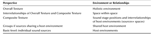
Any number of source host environments (sources+spaces) may occur simultaneously, and coexist within the same sound stage. All host environments (with their defining characteristics of width and depth, and source distance locations) are conceptually bound by the spatial impression of the holistic environment. As we recognize the sources plus their environments situated on the sound stage, we might begin to recognize spaces related to other spaces—just as the sources they host establish relationships, these spaces may have relationships to other spaces. On the sound stage sources+spaces are situated as parallel presences with other sources+spaces. Multiple environments are experienced simultaneously, just as multiple musical ideas and sound sources stream the materials of the track; in this way “the listener is aware of different types of space which cannot be resolved into a single setting” (Smalley 1997, 124). These simultaneous environments each carry their unique traits, supporting or enhancing their source and aesthetic ideas. The interrelationships of sources+spaces appear simultaneously with all of the other interactions of sources. A collage of host environments overlapping, sharing area, delineating, separating, etc. can readily established. A sense of function between host environments (sources+spaces) might emerge; as examples, a host environment might enhance its source to support the manner in which the source functions to cause tension and motion, other host environments might contribute to a sense of resolution or arrival, a shared environment might establish a context and character for groups of sources, and of course there are innumerable other possibilities.
Further, each host environment (being situated on the sound stage) is contained within the environment of the sound stage (the holistic environment). This creates an illusion of a space existing within another space (Moylan 2015, 209). The holistic environment contains all host environments; the host environments are nested within the holistic environment. This situation establishes relationships of host environments to the track’s overall space (Blaukopf 1971, 162).
This places the individual sound sources with their individual environments within the overall, perceived performance environment of the recording; this brings many spaces (sources+spaces) to ‘exist’ within the track’s holistic environment. Space within space and the hierarchy of environments allows for some unusual percepts—unusual, in that they defy what is possible in the physical world. Among these are:
- Simultaneous spaces, host environments existing side-by-side on the sound stage, with attributes distinguishing different types of spaces
- Overlapping spaces, where two spaces occupy the same area at their edges
- Embedded spaces, host environment emanating from within another physical space (perhaps the holistic environment)
- Multiple sound sources positioned at various distances within the same host environment (their common performance space)
Somehow the containment of all the track’s sources+spaces within its single overall environment is believable to listeners; one overarching place for the track can contain the many spaces (or worlds) from which diverse sources deliver and contribute their voice. Large spaces have no trouble fitting within small spaces in the world of a track. Again we find spatial qualities and relationships that do not align with life experiences, but that are readily accepted by the listener. Just as we allow ourselves to accept and believe the impossible within the invented worlds, storylines and actions of motion pictures, we accept the created and crafted worlds of records as the reality of a track. Each track re-invents physics and rewrites the laws of acoustics; any set of spatial qualities, dimensions and relationships can be found within the platform for track. The holistic environment often contains attributes of an environment that is significantly smaller than the spaces it contains (let alone the aggregate of all of those host environments). Individual host environments of sources may seem of enormous size, but fit into a tiny holistic space; this is a convention of space-within-space relationships.

Figure 8.10 Host Environments (sources and their spaces) on a sound stage; simultaneous spaces, overlapping spaces, spaces within space (host environments embedded within the holistic environment).
There is one additional level of environment, though this one is external to the track.
The listening environment and the listening process can enter the spatial hierarchy outside the track itself. The track is ‘heard’ by the listener from their own point of audition, and with their own sound system and listening sensibilities. They hear the track from within their own listening space. This space may add a layer to the experience, where “A listener might . . . apprehend a recording and experience a sense of a physical space, other than the one he was actually occupying” (Doyle 2005, 57). The sense of one physical space for the track and the listener in another may enter one’s perception. This separation might result in some detachment, perceiving the track at some point removed from the listener—a slightly removed position to one of significant separation. The environment produced by the playback system—or of headphones or earbuds—may become integral to the perception of the track, and bring attention to the listener’s point of audition. To a great extent, the impact of this playback environment will be heard similarly in other tracks played at similar loudness levels. A carefully located listening position at the peak of an equilateral triangle with the two loudspeakers placed to minimize room sound, with a balanced playback system will minimize the sound of their room and system, and may well make it negligible.
The Duality of Content and Character of Spaces
The contrast of content and character returns here; the attributes of spatial environments have physical properties (content) that establish a quality of character. Like timbre, environments can be conceived in two broad categories:
- a collection of measurable, physical, component parts or attributes that combine into a single, identifiable percept
- an overall impression (that at times acknowledges inner details) that results from the perception and interpretation of those physical attributes
Like timbre, environments can be approached to observe their content, or to observe their character. Indeed, to an extent, spaces may be conceived as timbres; the acoustic content of environments (spaces) combine in a gestalt, in conceptually the same way as the physical components of timbres. This might be conceived as a ‘timbre of the environment.’ In full, environments have a timbral quality comprised of component parts, plus integral spatial attributes, described later.
Environments are a collection of numerous physical components—with time, frequency, amplitude, and timbre dimensions—that represent its content. Environments are comprised of a complex, multidimensional set of sonic attributes, a collection of internal physical properties. Spaces can be largely observed through measureable parts—as just described. While these physical dimensions are scientifically measurable, they challenge aural analysis in many of the same ways of timbre analysis, but also in new ways. Spaces contain timbral information, but also discrete reflections and reverberation, and the time and dynamics matters they bring. Records contain spaces of various content; some of these spaces have a full set of attributes, others only one or a few. To observe environments, attention is focused inside to its component parts, to observe their attributes:
Environments can be approached as sound objects to evaluate content, just as we approached timbre—pulled out of context to unravel its subtle content.
We recognize spaces, and the character of spaces; environments carry qualities of ambience, spaciousness, size, and bear significance, connotations, associations, and more.
Environments can represent an aural image—as a singular character, or an overall characteristic. Spaces form an overall impression; environments are fused with the sound source and are also situated in an identifiable place of origin. Space assimilates into the source’s timbre, and contributes to any sonic representation of that source; we can experience space as links to places external to the track, and outside the listener. This conception of spatial environments often leads one toward descriptions of those overall qualities; descriptions of character and characteristics often result. The sonic representation is part of the sound’s spatial identity. Environments can often communicate conventional associations, and stand as symbols resonating outside the track. Environments “made it seem as though the music was coming from somewhere—from inside an enclosed architectural or natural space or ‘out of’ a specific geographical location—and this ‘somewhere’ was often semiotically highly volatile” (Doyle 2005, 5). The character of the overall quality that emerges from the perception and interpretation of the physical attributes establishes spaces and places that can produce subjective effects, can signify and represent, and can communicate to the listener.
The Sonic Content of Environments
Sounds in natural spaces interact with those spaces. The sound that results contains the timbral attributes of original sound source fused with a transformation of the sound brought about by the sonic imprint of the space. Rooms react to sound energy produced within; the results are a frequency response of the room, timings of reflections of the sound produced within, and dynamic contours of the room frequency response and the reflections. The interaction of the sound source and the environment produces a new, unique sound—one that has been transformed in timbre and provided with additional spatial properties. Throughout this explanation of the components of environments, one will recognize how timbre works with spatial properties (and loudness and time) to provide spaces with a unique profile. Engaging the sound of environments in deep listening, our attention is brought within the sound to hear these diverse and subtle dimensions.
The sound of a natural environment can be divided into three parts: direct sound, early reflections and reverberation. Environments within tracks may contain all of these parts and their attributes, or fewer—as they are often created, their content cannot be assumed. These three components (or whichever may be present) can be observed to identify the content of spaces.
Direct Sound and Pre-Delay
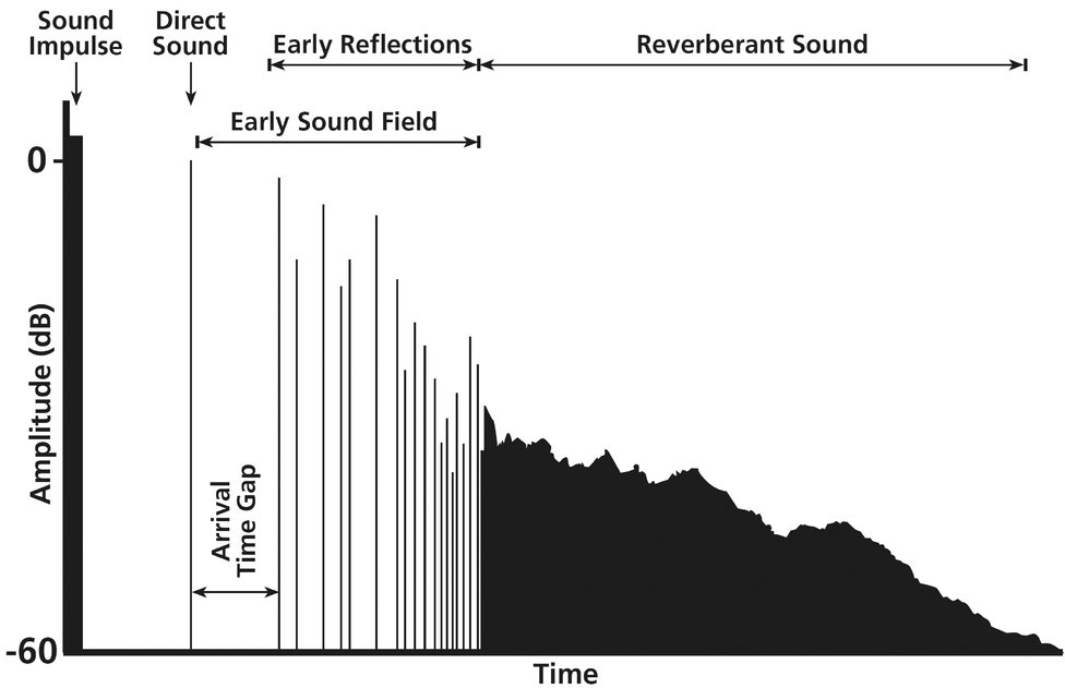
Figure 8.11 Unfolding time segments of environments, and types of reflections within environments.
Direct sound travels on the shortest distance between the source and the listener, and is therefore the first thing the listener hears. Direct sound delivers the information of the signal (sound source) to the listener in an uncontaminated form; it is unchanged by the environment, as it has yet to interact with it. A high proportion of direct sound provides clarity of the signal, and shares the attributes of sound in free space, because it has yet to interact with any boundaries. “Sound emanates from the source radially in all directions” (Everest & Pohlmann 2015, 97). In a free field, a source’s direct sound moves past the listener, never to return. With the same source in a room, the direct sound moves past the listener once in a direct path, then strikes a room boundary. As the source radiates in many (if not all) directions, these sounds reflect off one or many surfaces (walls, floor, ceiling, etc.) before arriving at the listener. The first of these reflections will arrive at the listener very shortly after the direct sound; these are early reflections.
The arrival time gap (also called pre-delay) is the time that separates the arrival of the direct sound and its first reflection. This time-length communicates important information about the size and dimensions of the space; it is determined by the distance the direct sound travels from the source to the reflective surface nearest the listener and then on to the listener. The time units of this distance play significant roles in our sense of the size of the space, and we have ‘learned’ the sounds of these time units, as blended into the overall quality of the source. For example, if conditions were right to allow sound to travel at 1000 feet per second (a rough approximation of what one might expect) the perception of a 50 ms delay places the length of distance the sound traveled at (very) roughly 50 feet (source to listener, inclusive of reflection path). Pre-delay alone is capable of adding depth to a sound source, simulating an environment.
Early Reflections and Early Time Field
Early reflections arrive at the listener within a window of time up to about 80 ms after the direct sound; another set of discrete reflections may arrive after this initial 35 to 80 ms, depending on the characteristics of the environment. The individual reflections will each have a potentially unique amplitude that is different from other reflections and that of the direct sound. The amplitude levels of early reflections are the result of distance travelled and the type of reflective surfaces; surfaces absorb some of the sound energy (varying by type of materials) and diminish the intensity of the reflection. The amount of energy that is removed when a sound strikes a surface material is its absorption coefficient; absorption coefficient varies with frequency. Early reflections also arrive from different directions (potentially from all directions); these different angles of arrival provide critical information on the location of the source within the space, the location of the listener within the space and also the size and geometry of the room.
Patterns of reflections are generated by spaces, providing a significant quality of its sonic imprint; these patterns combine spacing in time and of amplitude levels; they are ‘rhythms of reflections.’ Through this the early time field provides significant cues on the geometry of rooms, the source’s location within the room, and much more. The early time field exists in micro-timing, and often in rhythmic patterns and dynamic patterns; its short durations are less than 100 ms and as short as approximately 2 ms. Early time field reflections can simulate spaces (host environments) in themselves. Alone the reflections of an early time field can establish an illusion of a small space, or of unnatural spaces. Figure 8.12 illustrates the simplest reflection paths between the source and the listener; sound will continue to reflect around the space in more complex trajectories, establishing reverberant energy.
To summarize, early reflections bring the following traits; some will also appear within reverberation:
- Time delays from the arrival of the direct sound
- Amplitudes of reflections will differ from one another
- Frequency content of reflections is altered, from absorption by reflective materials
- Reflections arrive from different directions
- Patterns of reflections are established by repeated time delays and perhaps amplitude levels
Reverberation and Frequency Response
As sound continues to reflect in the enclosed space, it is reflected many times and arrives at the listener from all directions. The early time field dissolves into reverberation; the time this takes is a function of the size of the room, with smaller rooms taking a shorter amount of time to produce reverberation. Reverberant sound is a composite of the many reflections (from different reflection paths) arriving at the listener in close succession. The many reflections that comprise the reverberant sound are spaced very close in time to other reflections, and fuse into a single sonic impression. These many reflections are therefore perceived as a single entity. The time it takes for reverberant sound to die away is reverberation time, and is dependent upon both the size of the space and reflective materials.
Reverberation can be considered in three stages. The (1) initial portion of reverberant sound is the rate at which sound builds, and is determined by the time between reflections and absorption by materials and air; as more reflections and stronger reflections are generated by the space, the loudness level of the reverberation increases. This build-up will reach a (2) sustaining or steady-state level for the reverberant sound; this constant level is a balance between the amount of sound being produced in the environment and the amount being absorbed. This brings rooms with little absorption to have a higher steady-state level than rooms with more absorptive surfaces or longer distances between surfaces. Reverberant sound continues and decays after sound within the space stops. (3) Reverberation time is the rate (speed) of this decay; this is an important behavior that strongly reflects the character and content of a room. This rate is determined by the amount of reverberant energy continuing in the space, and is a product of the amount of absorption and the distance between reflective surfaces. Each time sound reflects in a room it loses some energy, absorbed during travel between surfaces and by contact with surfaces; between reflective surfaces, higher frequencies are absorbed faster than low frequencies. Surface materials absorb frequencies in different and unique proportions; some absorbing low frequencies more than high, etc. Longer reverberation times tend to be generated by larger spaces; sounds produced in spaces containing highly reflective materials of little absorptive capacity will take longer to decay.

Figure 8.12 Simple paths of reflected sound within an enclosed space.
With this we understand that reverberation will have different frequency content from the direct sound, brought about by loss of energy due to air absorption and also from uneven frequency absorption (and deflection) by reflective surfaces. Spaces typically have additional frequency content based on the geometry of reflective surfaces. Not all reflections travel in random directions; some reflections travel cyclically around a room, other reflections occur between opposing surfaces. These ‘standing waves’ are resonant modes that are spatially static; their pressure and velocity distributions stay within a certain subset of surfaces, are fixed in trajectory angle and wave length, and bring energy back to an original surface in a cyclic path. These paths exist for discrete frequencies that are determined by the geometry of the room, and bring significant variations of sound pressure levels around a room at those ‘modal frequencies.’ These are axial modes (between two surfaces), tangential modes (between four surfaces) and oblique modes (between all six surfaces). These modes might be conceived as ‘formant frequencies’ within the reverberant energy of an individual enclosed space.
The balance of the amount of direct sound to reverberant sound will shift with listener position relative to the sound source. In any space, there will be some distance between the listener and the source at which the reverberation will start to dominate. This distance (called ‘critical distance’) is highly variable depending on the size of the room and the materials of construction. This variability is precisely the reason reverberation (or more specifically ratio of direct to reverberant sound) is an ineffective measure for the perception distance location.
To summarize, reverberation contains the following traits. These traits can be extreme in created environments, and might appear in unnatural ways:
- Reverberation exhibits a dynamic shape that results from its build-up, sustain and decay; each stage has the potential for a dynamic profile, as each may contain changes in its dynamic level
- A density of reflections exists in reverberant sound; densities (number of reflections in a time unit) vary from one space to another
- Reverberant energy contains a different frequency spectrum (frequency response) from the direct sound, as a result of air and reflective surface absorption and of room modes
- Frequency response within reverberation is not static, and can exhibit considerable shifts throughout its duration; some frequency areas may get louder while others get softer, and at different speeds
The acoustic content of environments fuses together into a single percept. This overall quality of the environment is a gestalt; a complex overall experience that is different than the sum of these individual parts. These experiences—the inner workings of all environment attributes, or the overall quality of the environment—might be readily engaged by listeners in a general manner; for the goal of a recording analysis, heightened attention to details and relationships may reveal pertinent data. Denis Smalley (1997, 122) identified: “most listeners cannot easily appreciate space as an experience in itself. Spatial appreciation can be acquired by consciously listening to the spaces in works as distinct from regarding space as only . . . enhancement.” This manner of assessment and appreciating environmental content is a skill one can develop; one that can also be extended to the character of environments.
Observing Acoustic Content of Environments
Hearing the qualities of spaces requires directing attention to listening to subtle details of time, of activities in pitch/frequency areas, and and of dynamics—at a microscopic level—and also the resulting gestalt of the source+space sound. This is possible with some knowledge of what to listen for, and some guidance in how to hear it. The attributes of environments are subtle, and some are not perceivable as they are measured; in these instances, we perceive the results of the variable’s appearance or activity rather than the variable itself. Here we will engage the process and challenges of hearing the attributes of environments.
In observing these attributes, we are concerned with identifying (ultimately observing and understanding) the room’s sound separately from that of the sound source. We are attempting to understand the space in which the sound is resident—its sonic attributes, so that in the end we can examine how the source’s host environment contributes to its aesthetics.
The sonic signatures of environments are present and perceived, but difficult to segregate from the timbre that is exciting it. Environment characteristics are most clearly heard after the source stops abruptly; at that time a certain percentage of its reverb is audible—how much depends entirely on the attributes of the unique space. Within the context of the track, sources do not always stop abruptly; it is likely that in any track most sounds will not stop abruptly, as many naturally sustain until they are muted or decay below audible levels. Should a source stop abruptly in a track, it is very common for reverb information to be concealed by other sound sources.
This brings the analyst to need to engage the sound of the environment within context. A knowledge of the sound source, and the listener’s memory of that timbre are used to calculate ‘what is the direct sound (and its qualities)?’ and ‘how has it been altered?’. This extrapolates (estimates, applies an educated guess) toward identifying the physical content of the environment. This process is part past experience, and is in part an acquired skill; some detail is impossible to hear, so one directs attention to the result. One’s past experience of the timbre of the source allows one to recognize changes to spectrum (frequency response), changes to timbral detail (which is likely to diminish after the early time field); one’s past experiences of spaces allows a sense of size based on timbre within the early time field, as well as the duration of the reverberation and the ratio of direct to reverberant sound once the reverb cycle has reached saturation. In essence, we are trying to hear (recognize, determine) the dimensionality of the space and the content of the space’s timing and timbral signatures.
This process might extract the sound source from context—as a sound object—and observing the above qualities. Focusing on the perspective inside the sound, and out of the context of the track, allows isolation, and reduces distraction.
This is an appropriate time to remember that a significant percentage of environments encountered in tracks are artificial and/or incomplete. Observing the attributes of a host environment situated within a track, one often confronts contradictory percepts; further, many environments will not contain the full set or sequence of attributes found in natural environments. To observe content of room sounds in the detail they can be measured is impossible; it is unrealistic to attempt to identify many percepts with precision. To observe the basic traits of dominant content is possible, though, and can yield information significant to a track. Table 8.9 presents a typology table for the content of environments; it can be modified to complement individual environments, and the values it recognizes can be generalized when specifics cannot be identified (or when they are not needed for an analysis).
The content of the environment as an overall percept allows most direct and simplest access to observing an environment. This can be approached in three parts. First, one can approach the reverberation plus early time field as a single gesture—one with a dynamic contour, a duration, and a sense of density. This data would in itself be significant in defining the environment. Second is the frequency response (or spectrum) of the environment; remembering that the space reacts to sound energy that is produced within it, certain frequencies are emphasized and some attenuated. These can be identified related to pitch register, to obtain data on, for example, whether the environment boosts low frequency information and by how much (as in ‘the Low pitch register is moderately emphasized’). Third is the dynamic relationship between the direct sound and the reverberant/
Table 8.9 Content typology table for observation of individual host environments; may also be applied (in whole or in part) to observing the content of holistic environments.
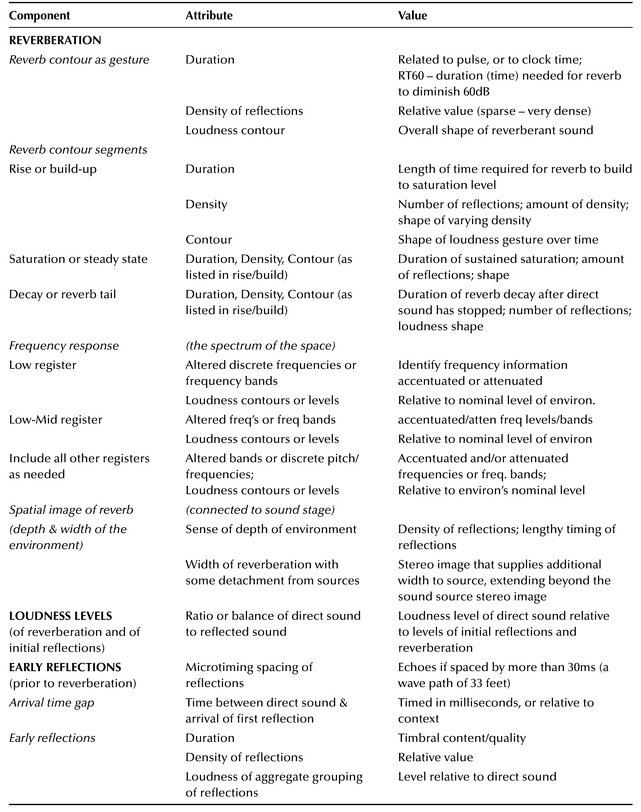
environment sound; this is a relative proportion (‘direct sound is slightly louder than the reverb’). The higher the proportion of reflected sound to direct sound, the more the level of distinguishability of the sound source diminishes—resulting in diminishing the level of timbral detail of the source (indication of distance as well as space). Time-related observations can be calculated against the track’s metric pulse (for some environments, but certainly not all); durations of reverberation can be calculated against clock time as well. If necessary, general time comments such as ‘short’ or ‘long’ might be a starting point, and ‘shorter-than’ might begin a comparison with another environment—either within or outside the track.
Observations of greater detail might be accomplished, as might be appropriate for the analysis—or the skill level of the analyst. Explanations of these more detailed observations and processes follow.
Already noted above, the arrival of the first reflection provides important indication of the size of the environment. This time unit is very often smaller than the threshold of pitch fusion (50 ms) and typically within the threshold of order (3 to 25 ms).21 Therefore, the reflection is not perceived individually, but rather as part of the timbre of the source. This percept manifests as an alteration of timbre brought about by time; we can learn to recognize this subtle alteration as timbre should we wish, as we already process this information to identify room size. A single short-duration reflection is commonly used to add substance to sound sources, particularly vocals. Further, this single reflection alone is enough to provide the impression of an environment size and character.
The arrival of multiple reflections in the early time field (ETF) has three important factors for observations. The first two are reflected in the overall timbre of the source, though their origins might be recognized as related to density and loudness. First (1), it can bring a sense of density, or an amount of activity within its very short time window; a relative density (‘sparse’ to ‘very dense’) can be noted as part of the observation. Second (2), the loudness levels of all reflections in the ETF can provide an impression of proportion of direct sound to reflected sound; this ratio can be observed on a general scale, to help define content. The ETF will be primarily recognized as a shift in the timbre of the sound source; this timbre shift might occupy a significant portion of the sound’s onset. These reflections can provide further information on the size of the space, and the position of the listener and the positioning of the sound source within the space. The timbral alterations brought about by these ETF reflections are subtle, and difficult to define. Third (3), of significance here is the duration of the ETF, as it separates the arrival of the first reflection from the beginning of reverberation. Should it not be possible to calculate a duration of the ETF, one might acquire a sense of how quickly the reverberant energy begins, and provide a general comparison to a known room of similar size (for example, “the ETF appears to be similar to that of my church”).
The three stages of reverberation (build-up, sustain and decay) might be identifiable, but may be obscured or simply not present in others. When present, each might be observed for their duration, density of reflections and dynamic relationship to the direct sound. The overall reverberation time is an important element of the environment, and can be calculated in clock time or against the pulse of the track. The frequency ranges emphasized and attenuated are apparent within the reverberant energy; some ranges will have different reverberation times than others. With practice one might recognize these when they are present (and prominent).
Summarizing all of this: the process of observing the content of spaces (environments) acknowledges that the attributes of environments only exist when they are excited by the sound of the source(s) performing within it. The source’s different performed pitches and the variety of frequency content they contain reveal certain characteristics of environments slowly over time and many different soundings. Other data is more consistent over the source’s frequency range.
The typology table of Table 8.9 lists the attributes with their value types of spaces. Hearing these broader attributes of spaces will be readily accessible to many readers; it can start with the broadest and most apparent qualities of reverberation, especially the residue after the direct sound has concluded. This process can then progress to the most detailed and thorough observations, such as microtiming (millisecond delays heard as timbres of time increments) of the early reflections.
These have been consolidated into four stages, each containing several attributes:
- Reverberation: (a) duration (RT60), (b) density of reflections, (c) loudness and density contour of the reverberation divided into three segments (Praxis Study 8.6)
- Reverberation: (a) frequency response (frequency bands or discrete frequencies that are accentuated or attenuated by the environment), (b) loudness levels (the ratio or balance of the direct sound to reflected sound) (Praxis Study 8.7)
- Early reflections: (a) arrival time gap (time before the arrival of the first reflection), (b) early time field (duration before beginning of reverb, density of reflections, loudness of ETF reflections in aggregate compared to direct sound) (Praxis Study 8.8)
- Environments: (a) cues that at times establish a sense of depth to the source+space image, and (b) potential of reverberation sound to extend the width of an image with the reverberation heard as separated from and around the direct sound of the source (Praxis Study 8.9)
As with timbre, the level of detail within observations can shift with the goals of the analysis; all attributes of an environment do not need to be revealed, indeed that would be great effort that would often produce little relevant data for many tracks (or sources). Selective observations will hold value when they reflect those components that provide the environment its uniqueness and that recognize its prominent traits.
Character of Environments
Spaces (including echo and reverberation) produce “powerful subjective effects in listeners” (Doyle 2005, 31). These effects are embedded in the character of environments, and linked to semiotics and interpretation. Relations exist between the sounds of spaces within tracks and “what those spaces signify to those producing and hearing the sounds in specific sociocultural contexts.”22 Engaging a study of spatial semiotics, or developing a vocabulary for the character of environments are well beyond the limitations of this writing, though some approach to describing character must be attempted here, in order to incorporate this important spatial trait into the recording analysis.
Character is inherently a description and an interpretation; just as encountered with timbre in Chapter 7. Character can be defined to address the affects and effects of, and the activities within, its content. As character can engage the subjectivities and quasi-subjectivity of what spaces elicit within individuals, describing character pulls the analyst into the equation—along with their biases, knowledge, experience, abilities and more. Spaces carry cultural meanings, associations, connotations, etc.; approaching descriptions from cultural norms allows the opportunity for communication with a wider audience. The potentials for individual interpretation and for differing meanings within social groups and subcultures, let alone between cultures, ensure any approach will be fraught with difficulties. Still, there is some notion of common ground—the sound itself.
Descriptions that emerge from the examination of an environment’s physical content carry a common ground. The interpretation of the content may differ between individuals, but the sound itself with be largely the same (assuming similar playback variables). Describing the attributes of the sound provides a useful starting point, and can allow the description to unfold with relevant information. One can then extend observations to other areas. Just as with timbre, a description of an environment that provides a clear indication of the nature, context, content and associations (as appropriate) is likely to be most successful.
The term ‘ambience’ has been used to describe varying qualities of the tracks, and sometimes used synonymously with reverberation.23 Ambience is the sonic presence of a place, and as such is interpreted. In some areas of production (such as classical music recording, television productions and films), ambience is room sound (often called ‘room tone’); it is the sound of the space where a recording is being made. ‘Ambience’ can describe the sound of the recording space itself—alone and void of any sonic activity. This concept can be transferred to spaces—real or virtual—within the track. The sound of the room, separate from the sound of the source sounding within the room, may bring environments to be sound objects that can be frozen in time for examination out of context as content; environments can also be examined as events changing in real time and observed in context of the track as character. In this writing, ‘ambience’ is used to denote an affective response to the overall character of an environment, within a broad cultural context (in as much as it might be possible). This is an extension of the common use of ‘ambience’ to represent the mood, feeling, aura or atmosphere of a place.
Our approach to the character of environments will (1) seek to recognize their overall qualities and to describe them relative to the context of the track; this might include addressing some portion of the physical attributes of a space. Character descriptions will also be (2) relative to how an environment might be situated culturally—and perhaps how the listener interprets them.
Qualities that elicit impressions of character are innumerable, including the most ethereal described under ambience. Other qualities might directly engage the space itself, often involving past experiences to interpret the physical dimensions one perceives. A listener may compare the environment they are hearing with what they have previously experienced (and remember); they make connections and comparisons, perhaps associations. A comparison might engage the size of the heard space (‘this space is larger than space A and similar in size to space D’) or the types of spaces they have experienced (lecture halls, hallways, concert halls, rooms, etc.).
Spaciousness is a spatial impression of an environment. It describes the sense of open space around a sound source, a sense of expanse. Spaciousness is an impression of the size of a room, and also a sense of the amount and type of reflection within the space (Rumsey 2001, 38). Rooms with longer times between direct sound and early reflections, especially those arriving from the sides, have a greater sense of openness or spaciousness. The sense of spaciousness is commonly a dominant characteristic, giving the host environment a sense of depth extending behind the location of the sound source and a sense of breadth or width to the environment, as it can extend to either side of the lateral location of the source image.
Observing the Character of Environments
The process of observing environment character pulls together observations of the physical content of the space with what those dimensions elicit in the listener. Interpretations, as we have noted, are potential grounds for overly personalized observations; here, again, it is encouraged that cultural norms be emphasized in observations. Personalized observations, if used, are best identified as such, so as not to imply they are those the reader might share.
Environment character situates and colors the performance within a space, and we recognize its impact on the source within the context of the track. Character also embraces outside matters that may arise—it has rhetorical forms (just as does timbre): semiotics, extramusical connotations, connections to real spaces within one’s experiences, and more. The size of a space carries connotation and meaning, as well as sonic properties. The affects of spaces set a scene of the track, or of each of its sources—ambience, mood, aura, level of tension, and more. The character (and content) of environments can generate new meanings for musical materials and sources. Brøvig-Hanssen & Danielsen (2016, 134) observe that
Placing a sound within a space provides it with added meaning (enhance or support the meaning that is present), and the space itself can transform a source and its materials into something different. Spaces can minimize and can expand a source, or they can dominate a source. Still, the sound of a space does not exist without the source that sounds within it, and the two have a significant bond between them.
Table 8.10 Potential typology attributes (with values) of the character of individual host environments; may be adapted for observing character of holistic environments.
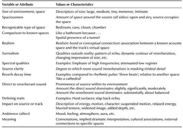
Table 8.10 presents a general typology of attributes (with related values) of the character of an environment. This is presented as a point of departure. Certainly some tracks will contain spaces that require observation of additional attributes; those will be identified as data collection unfolds. This table does present an approach to organizing a description of character based on content and utilizing listener experience.
These all have an element of subjectivity stemming from interpretation, experience and exposure. Still, this typology could communicate a certain degree of objectivity around some commonality. Different analysts will engage these attributes in varying ways depending on skill and experience; the reader will interpret the analyst’s prose through their own set of experiences and level of knowledge and listening skill levels. As an interpretation, character carries the inherent subjectivity of the analyst’s biases; as with the character of timbre, the most useful interpretations minimize personal biases and emphasize those that are cultural, and that engage pertinent qualities of the track itself.
The aesthetic and affect-related descriptions of character include those that the physical content elicit, and the analyst’s perception of the ambience’s qualities as it is situated within the context of the track. Importantly, character is the sound of the environment as it contributes to the sound source’s gestalt, as it contributes to the sound stage and the track, and more. In this way, describing the character of an environment is an evaluation; a step undertaken after observations of content, by further observing and evaluating the space within the context of the track.
Observing Holistic Environments
Observing the holistic environment may be directed toward an environment that has been applied to the track—accomplished by routing the mix through a reverb/environment simulation processor or plug-in. Should an applied environment be absent (which is most common), the holistic environment is approached ‘holistically’ (as a whole with interdependent parts), by observing the spaces of all sources, perhaps emphasizing those that provide the track with its strongest qualities. Observing the holistic environment involves both content and character. As in host environments, observing content will provide some degree of context toward interpreting a definition of its character.
Remembering a track’s holistic environment is a single impression of space—the track’s space—we recognize it contains all host environments. It encapsulates the many potentially disparate spatial impressions, which interact within the unique mix of the track, and it may also reflect them.
In records, a holistic environment is rarely a real space; it is also rarely even a single, fabricated virtual space. Rather, the holistic space of the track is the result of a blending of numerous factors, and is to varying degrees influenced by all sources and materials. The holistic environment is most likely to manifest its sonic impression with some of the following content attributes:
- Frequency levels or regions that are consistently accentuated or attenuated, thus altering the timbral balance of the track, along with the manner(s) in which these alterations unfold over time (dynamic contours)
- Reverberation time and density of reflections
- Ratio of levels comparing direct sound to reverberant sound
- Early time field arrival time gap and spacing of early reflections
- Dimensions of the sound stage (depth and lateral boundaries)
Attributes of the source host environments contribute to the impression of the holistic environment; for the majority of records the holistic environment is an overall impression generated by the content/character and the interactions of all host environments and their sources. There can be no formula to engage the process of identifying the quality of the holistic environment—each track is unique, and to some degree will generate its holistic environment in its own way. Some portion is an interpretation, an impression of character and surface features; some portion is the dominant or prominent or unique spatial attributes within the overall sound. The source host environments will not all contribute equally; the track itself will offer up what defines its holistic environment. The most significant or prominent sources may serve a dominant role, or they may be overshadowed by a unique environmental quality in a secondary source; the contextual layer of a track might establish a sonic space against which all other activity is calculated. Every track will be at least somewhat unique in how its holistic environment is formed—as well as its content and character.
The defining questions are: What is the environment in which this unique track is housed? What are its sonic attributes? To what extent is it an audible presence or a conceptual context?
The typology tables for content of environments and character of environments can be used to observe holistic environments. The attributes of each table will be somewhat unique for each track. The process of exploring the holistic environment to engage those tables’ attributes will provide the analyst guidance.
In talking about the environment of the soundbox representing Prince’s “Kiss” (1986), Brøvig-Hanssen & Danielsen (2013, 76) identify qualities and dimensions of the track’s holistic environment, as having the width and resonance characteristics of a large hall, while the depth reflects a small, “‘dry’ or dampened space.” Their assessment continues: “this single space comes forth as surreal . . . the hyper-presence and lack of depth imply a small space with almost no reverberation, but the high intensity and voluminous sound imply a larger, resonant one.” Allan Moore (2001, 163) is discussing common traits of holistic environments of U2 when he identifies:
Both examples acknowledge and describe the content of this overall space of the track; note, they examine frequency content along with time delay and reverberation as attributes of the experience.
The character of a holistic environment represents the listener’s (analyst’s) impressions of the overall spatial identity of the track, as a global character trait. This impression is elicited through the experience of the track—an impression that can shift somewhat with re-hearings, further observation and evaluation. Like all thoughtful interpretations, the interpretation of the holistic environment is a work in progress, with new observations and discoveries building on the former. This process is on-going, and continual for the attentive listener.
CONCLUSION
Spatial properties provide the track with a sense of place and space, at multiple levels of perspective.
Each sound source in the track contains and projects a spatial identity. Spatial identities of sources can be defined by their lateral and distance positioning, and the attributes of its host environment, though this would be incomplete. The spatial identity of sources contains a semiotic level, a functioning role within the track’s materials, and unique, multidimensional presence within the track. A dimensionality of the spatial identity is also generated by the character of its environment, and by how its distance, size and lateral position can elicit powerful subjective associations and effects within listeners. The spatial identity of a sound source provides it with a place—a place that coexists with the spaces of every other sound source (overlapping, situated side-by-side, or separated by some variable space), as all sources+spaces are resident in the sound stage.
The track has a spatial identity as well. It is one of the dimensions of the track’s crystallized form—which will be revisited in greater detail in Chapter 9.