Figure 6.1. p-value associated with the slope on casino employees (CE) in the Stoke’s Lodge multiple regression example.
Chapter 6 Preview
When you have completed reading this chapter you will be able to:
• Identify the five steps involved in evaluating a multiple regression model.
• Evaluate whether a multiple regression model makes logical sense.
• Check for statistical significance of all slope terms in a multiple regression model.
• Use the p-value method to evaluate statistical significance.
• Evaluate the explanatory power of a multiple regression model.
• Test the overall significance of a multiple regression model.
• Check for serial correlation in multiple regression models with time-series data.
• Check for multicollinearity in multiple regression models.
• Make point and interval estimates based on a multiple regression model.
Introduction
At this point, you are familiar with the basics of ordinary least squares (OLS) simple regression analysis where you use one independent variable to explain variation in the dependent variable. You know how to run simple regression in Excel, evaluate simple regression models using the four-step procedure, and make point or interval estimates of the dependent variable in a simple regression model based on some given value of the independent variable. In this chapter, you will learn how to expand simple regression models to include multiple independent variables. When doing multiple regression there are some modifications and additions needed to the four-step evaluation procedure discussed previously.
Multiple Linear Regression
In many (perhaps most) applications, the dependent variable of interest is a function of more than one independent variable. That is, there is more than one independent variable that can be used to explain variation in the dependent variable. In such cases, a form of OLS regression called multiple linear regression is appropriate. This is a straightforward extension of simple linear regression and is built upon the same basic set of assumptions. The general form of the multiple linear regression model is:
![]()
and the regression equation becomes:
![]()
where Y represents the dependent variable and Xi represent each of the k different independent variables. The intercept, or constant, term in the regression is a and the bi terms represent the slope, or rate of change, associated with each of the k independent variables in the model.
The addition of more independent variables to the basic regression model is almost always helpful in developing better models of economic and business relationships. Doing so, however, does mean a bit of modification to the four-step evaluation process used to evaluate simple regression models with only one independent variable (discussed in chapter 4). You will recall that those four steps involved answering these questions:
1. Does the model make sense? That is, is it consistent with a logical view of the situation being investigated?
2. Is there a statistically significant relationship between the dependent and independent variables?
3. What percentage of the variation in the dependent variable does the regression model explain?
4. Is there a problem of serial correlation among the error terms in the model?
For multiple regression analysis, you need to add a fifth question:
5. Is there multicollinearity among the independent variables? Multicollinearity occurs when two or more of the independent variables in multiple regression are highly correlated with each other.
Let us now consider each of these five questions and how they can be answered for a specific multiple regression model.
Stoke’s Lodge Multiple Linear Regression Example
Reconsider the simple regression analysis that you were introduced to in chapter 4 on monthly room occupancy (MRO) at Stoke’s Lodge. Average gas price (GP) in dollars per gallon per month was the only independent variable in the model and you obtained the following regression equation:
![]()
However, you know that during the time period being considered there was a considerable expansion in the number of casinos in the State where Stoke’s Lodge is located, most of which have integrated lodging facilities available. So, you decide to collect monthly data from January 2002 to May 2010 on the number of casino employees (CEs) working in the State (in thousands) because you want to include this as an additional independent variable in your regression model. Table 6.1 shows a shortened section (the first 24 observations) of the data set.
Table 6.1. Monthly Data for Stoke’s Lodge Occupancy, Average Gas Price, and Number of Casino Employees (The First Two Years Only)
|
Date |
Monthly room occupancy (MRO) |
Average monthly gas price (GP) |
Monthly casino employees in thousands (CE) |
|
Jan-02 |
6,575 |
1.35 |
5.3 |
|
Feb-02 |
7,614 |
1.46 |
5.2 |
|
Mar-02 |
7,565 |
1.55 |
5.2 |
|
Apr-02 |
7,940 |
1.45 |
5.2 |
|
May-02 |
7,713 |
1.52 |
5.1 |
|
Jun-02 |
9,110 |
1.81 |
5.0 |
|
Jul-02 |
10,408 |
1.57 |
5.0 |
|
Aug-02 |
9,862 |
1.45 |
5.0 |
|
Sep-02 |
9,718 |
1.60 |
5.1 |
|
Oct-02 |
8,354 |
1.57 |
5.8 |
|
Nov-02 |
6,442 |
1.56 |
6.6 |
|
Dec-02 |
6,379 |
1.46 |
6.4 |
|
Jan-03 |
5,585 |
1.51 |
6.4 |
|
Feb-03 |
6,032 |
1.49 |
6.4 |
|
Mar-03 |
8,739 |
1.43 |
6.3 |
|
Apr-03 |
7,628 |
1.62 |
6.3 |
|
May-03 |
9,234 |
1.83 |
6.3 |
|
Jun-03 |
11,144 |
1.63 |
6.3 |
|
Jul-03 |
8,986 |
1.36 |
6.2 |
|
Aug-03 |
10,303 |
1.52 |
6.2 |
|
Sep-03 |
8,480 |
1.67 |
6.2 |
|
Oct-03 |
9,135 |
1.28 |
6.2 |
|
Nov-03 |
6,793 |
1.17 |
6.2 |
|
Dec-03 |
5,735 |
1.13 |
6.4 |
The results of the multiple regression analysis can be found in Table 6.2. The regression equation is as follows:
![]()
Notice that there is a slope term associated with gas price (–1,097.686) and another slope term associated with casino employees (–1,013.646). Let’s evaluate this model!
Evaluation Step 1: Evaluate Whether the Model Makes Sense
First and foremost, your regression model still must be logical. There is nothing different about this step of the evaluation procedure except for the fact that you have multiple independent variables and therefore you must evaluate the sign of each of the slope terms in the model to make sure that they each make logical sense.
For the Stoke’s Lodge multiple regression model, a negative slope is still expected for gas price because higher gas prices will deter people from traveling and therefore room occupancy is expected to decline. But, what about the slope term on casino employees? The idea here is that the expansion of the casino industry has caused a decline in the occupancy at Stoke’s Lodge because these new casinos have integrated lodging facilities and are considered to be competitive. Therefore, a negative slope is also expected for casino employees because more employees working in the casino industry indicates an increase in competition and should result in a decline in occupancy at Stoke’s Lodge. The OLS equation was found to be:
![]()
We see that the signs on both GP and CE are indeed negative and so this model does make logical sense.
Evaluation Step 2: Check For Statistical Significance
Similar to step 1, there is little difference in this step of the evaluation procedure except for the fact that you have multiple independent variables and therefore you must check for statistical significance of each of the slope terms in the model. Therefore, you will have multiple hypotheses to test. However, in multiple linear regression, the appropriate number of degrees of freedom (df) is: df = n – (k + 1), where n equals the number of observations used in your sample and k is the number of independent variables used in the model.
Recalling from chapter 4 that the statistical test of significance of a regression slope can take any of the following three forms depending on what you are trying to determine:
Case 1: This form is appropriate when you are testing for the existence of any linear functional relationship between Y and X.

Case 2: This form is appropriate if you think that the relationship between Y and X is an inverse one.

Case 3: This form is appropriate if you think that the relationship between Y and X is a direct one.

For the Stoke’s Lodge example, you determined that the model makes sense because the slope term on both gas price (GP) casino employees (CE) was negative. But, are these slope terms significantly less than zero? Since there is an expected inverse relationship between monthly hotel room occupancy (MRO) and gas price (GP) a one-tailed test as described in Case 2 is appropriate. Similarly, since there is an expected inverse relationship between monthly hotel room occupancy (MRO) and casino employees (CE) a one-tailed test as described in Case 2 is appropriate for this independent variable as well.
First, let’s test for significance on the slope term on gas price (GP). The null hypothesis is that the slope is greater than or equal to zero (H0 : b ≥ 0). The alternative hypothesis is that the slope is less than zero (H1 : b < 0). Excel results showed that the standard error for the slope on GP is 251.265, so you can calculate tc for GP as follows:

There were 101 observations in the data set and two independent variables in the model, so df = n – (k + 1) = 101 – (2 + 1) = 98. Looking at the t-table in Appendix 4B, find the row for 98 df and the column for a one-tailed test with a level of significance of 0.05, and you get the critical value for t to be 1.658.1 Thus, in this case the absolute value of tc for GP (|–4.369|) is greater than the critical t-table value (1.658) and you have enough statistical evidence to reject the null hypothesis. Therefore, you conclude that there is a statistically significant negative relationship between MRO and GP at the 5% level of significance (a = 0.05).
Next, let’s test for significance of the slope term for casino employees (CE). The null hypothesis is that the slope is greater than or equal to zero (H0 : b ≥ 0). The alternative hypothesis is that the slope is less than zero (H1 : b < 0). Excel results showed that the standard error for the slope on CE is 344.959, so you can calculate tc for CE as follows:

Again, there were 101 observations in the data set and two independent variables in the model, so df = n – (k + 1) = 101 – (2 + 1) = 98. It is a one-tailed test and the level of significance is still 0.05 so the critical t-table value is still the same as found above for the hypothesis test on gas price. Thus, in this case the absolute value of tc for CE (|–2.938|) is greater than the critical t-table value (1.658) and you have enough statistical evidence to reject the null. Therefore, you conclude that there is a statistically significant negative relationship between MRO and CE at the 5% level of significance (a = 0.05).
Therefore, gas price (GP) and casino employees (CE) are both considered statistically significant in their negative relationship with occupancy (MRO) at the 95% confidence level.
P-values: A Short-Cut to Determining Statistical Significance
You may have noticed that there is a column in the Excel regression computer output next to the t-stat that is labeled “p-value”. The p-value can be used as a quick way to evaluate statistical significance and can be used as an alternative to comparing the computed test statistic, tc , with the critical t-table value(s). It applies to either simple or multiple regression analysis.
The p-value is the probability of observing another computed test statistic or t-stat that is more extreme (either positive or negative) than the one computed for your sample. Therefore, the smaller the p-value, the more support for the alternative hypothesis. That is, a small p-value implies a small chance of ever obtaining another sample with a slope term more statistically different from zero than the slope term is for your sample.
Consider the p-value for casino employees (CE) which is 0.004. This means that there is a 0.4% probability of observing another computed t-stat that is more extreme than the one computed for this sample (tc = -2.938). This probability is illustrated by the shaded regions of the graph in Figure 6.1.
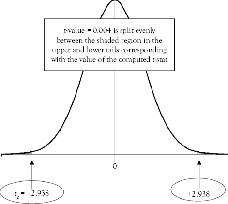
The shaded regions in Figure 6.1 would be relevant if you were performing a two-tailed test (Case 1) and just concerned about whether the slope of CE was statistically different (either higher or lower) from zero. However, because you are performing a left-tailed test (Case 2) for the slope on CE and only concerned about whether the slope is statistically less than zero you must divide the p-value by 2 because only the probability in the left tail of the distribution is relevant. Similarly, when performing a right-tailed test (Case 3) you must divide the p-value by 2 because only the probability in the right tail of the distribution is relevant as you are testing whether the slope is statistically greater than zero. In Table 6.2, a column is created next to the p-value labeled “p/2” that can be used when evaluating significance for one-tailed tests (Case 2 or Case 3).
Table 6.2. Regression Results for Stoke’s Lodge Occupancy Multiple Regression
|
Regression statistics |
|||||
|
Multiple R |
0.466 |
DW = 0.7303 |
|
||
|
R-square |
0.217 |
||||
|
Adjusted R-square |
0.201 |
||||
|
Standard error |
1,611.772 |
||||
|
Observations |
101 |
||||
|
ANOVA |
|||||
|
|
df |
SS |
MS |
F |
Sig F |
|
Regression |
2 |
70,491,333 |
35,245,666.7 |
13.567 |
0.000 |
|
Residual |
98 |
254,585,374 |
2,597,809.94 |
||
|
Total |
100 |
325,076,708 |
|||
|
|
Coefficients |
Standard error |
t Stat |
p-Value |
P/2 |
|
Intercept |
15,484.483 |
2,162.820 |
7.159 |
0.000 |
0.000 |
|
GP |
–1,097.686 |
251.265 |
–4.369 |
0.000 |
0.000 |
|
CE |
–1,013.646 |
344.959 |
–2.938 |
0.004 |
0.002 |
So, you may be wondering how the p-value (two-tailed test) or p-value /2 (one-tailed test) helps you to determine statistical significance. A simple comparison is made with the level of significance. For situations such as that described in Case 1, the null hypothesis is rejected and you conclude that the true slope is different from zero if the p-value is less than or equal to the desired level of significance, a. For situations such as that described in Case 2, the null hypothesis is rejected and you conclude that the true slope is less than zero if the p-value/2 is less than or equal to the level of significance, a. Finally, for situations such as that described in Case 3, the null hypothesis is rejected and you conclude that the true slope is greater than zero if the p-value/2 is less than or equal to the level of significance, a. This assumes that you have already passed test one, so you have a logical model. Again, if you do not satisfy evaluation step one nothing else matters.
Now, back to the Stoke’s Lodge multiple regression example where you expected both the slope on gas price (GP) and the slope on casino employees (CE) to be negative and therefore needed to perform left-tailed tests to determine statistical significance. As a result, the p/2 is the relevant statistic in each case and can be found in the Excel regression output in Table 6.2. The p/2 is 0.000 for GP and 0.002 for CE. Since both values are less than the level of significance (a = 0.05), the null hypothesis is rejected in both instances and both the slope for GP and CE are statistically less than zero (significant), at a 95% confidence level.
Evaluation Step 3: Determine the Explanatory Power of the Model
The Adjusted R2
When analyzing multiple regression models, the adjusted coefficient of determination (adj-R2) is used rather than the unadjusted coefficient of determination (R2) that is used in simple regression.2 The reason for the adjustment is due to the fact that the unadjusted R2 will always increase as any new independent variable is added to the model, whether the variable is relevant or not. On the other hand, the adj-R2 may or may not increase when a new independent variable is added to the model. Thus, in interpreting multiple linear regression results one should always look at the adjusted coefficient of determination (adj-R2) in order to evaluate the explanatory power of the model. The adj-R2 still gives the percentage of the variation in the dependent variable (Y) that is explained by the regression model.
For the Stoke’s Lodge hotel occupancy model, the adjusted coefficient of determination is 0.201 (See Table 6.2).3 This means that 20.1% of the variation in monthly room occupancy (the dependent variable) is explained by the model. In the bivariate (simple) regression in chapter 4 for Stoke’s Lodge you saw that the explanatory power was only 14.8%. Now you see that by adding an additional independent variable the explanatory power has increased to 20.1%. In an appendix to chapter 8 you will see that this can be improved to about 83%.
Overall Test of Significance for Multiple Regression
A test of the overall significance of a regression equation can be performed for multiple regression and is related to the coefficient of determination. It is sometimes referred to as the F-test. The null hypothesis is that there is no relationship between the dependent variable and the set of independent variables. That is, ![]() (i.e., all slope terms are simultaneously equal to zero).4 The alternative hypothesis is that all slope terms are not simultaneously equal to zero and denoted by
(i.e., all slope terms are simultaneously equal to zero).4 The alternative hypothesis is that all slope terms are not simultaneously equal to zero and denoted by ![]() .5
.5
The computed test statistic for the test of overall significance is the F-statistic, Fc, and can be computed as follows:
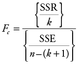
where SSR is the sum of squared regression (explained variation) and measures the amount of the variation in the dependent variable (Y ) that is explained by the set of independent variables, SSE is the sum of squared residuals, or errors, (unexplained variation) and measures the amount of the variation in the dependent variable (Y ) that is explained by one or more variables not considered in our regression model, k is the number of independent variables in the model, and n is the total number of observations in the sample. The F-statistic, Fc, can be found as a standard part of most computer regression outputs. Table 6.2 shows that Fc is equal to 13.567 for the Stoke’s Lodge multiple regression example. You see, in Table 6.2, that this statistic is part of an “ANOVA” table. ANOVA refers to analysis of variance, which is another statistical tool.
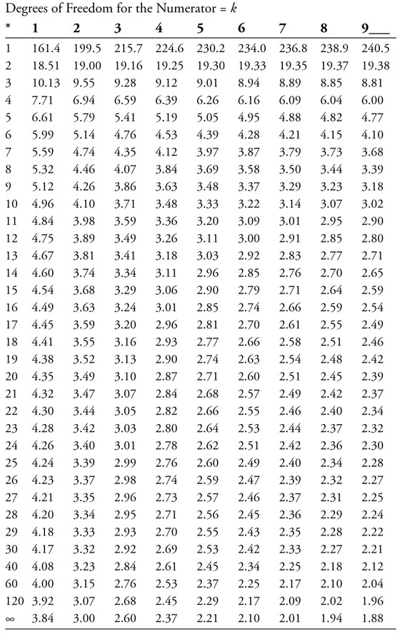
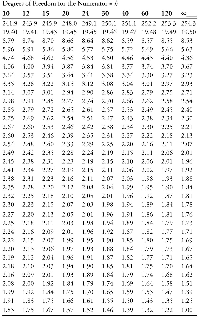
The critical value for the F-test can be found using the F-distribution table (F-table for a 5% level of significance is shown in Appendix 6A). The appropriate degrees of freedom (df) are equal to k for the numerator and n – (k + 1) for the denominator. The critical value is then found at the intersection of the column and row corresponding to these values. In the Stoke’s Lodge multiple regression example, the df for the numerator is equal to k = 2 and the df for the denominator is equal to n – (k + 1) = 101 – (2 + 1) = 98. So, the critical F-table value is 3.07.6
If the computed F-statistic, Fc, is greater than or equal to the critical value from the F-table, the null hypothesis is rejected. Also, note that a p-value is given in the Excel computer output next to the computed F-statistic. If this p-value is less than or equal to the desired level of significance, a, this also tells you that the null can be rejected. If the null hypothesis is rejected, you can conclude that overall the regression function does show a statistically significant relationship between the dependent variable and the set of independent variables. In the case of Stoke’s Lodge, the computed Fc (13.567) is greater than the critical F-table value (3.07) and/or the p-value (0.000) is less than the desired level of significance (0.05); therefore, the null hypothesis is rejected and you conclude that overall the regression model is significant at a 95% confidence level.
Evaluation Step 4: Check for Serial Correlation
The procedure used to check for serial correlation in multiple regression analysis is exactly the same as described in chapter 4 for simple regression analysis. There is no difference! Recall, since MRO is time-series data, a check for serial correlation is necessary for the Stoke’s Lodge multiple regression example. The DW statistic is calculated to be 0.7303. To formally evaluate the DW statistic for the MRO regression you know that n = 101 (number of observations) and k = 2 (number of independent variables). From the DW table (Appendix 4C), you find the lower bound of DW = 1.391 and the upper bound of DW = 1.600.7 Test 6 in Table 4.2is satisfied, since the calculated DW statistic of 0.7303 is less than the lower bound (1.391) from the DW table. Therefore, positive serial correlation still exists in the multiple regression model for MRO.8 Remember that serial correlation does not affect the regression coefficients but can inflate the calculated t-ratios.
Evaluation Step 5: Check for Multicollinearity
Multicollinearity occurs when two or more of the independent variables in multiple regression are highly correlated with one another. When multicollinearity exists, the regression results may not be reliable in that the values of the slope terms may be incorrectly estimated. The existence of multicollinearity may be a reason why the signs of the slope terms in a model fail to make logical sense. This would be an example of over specification of a regression model.
When multicollinearity exists, it does not necessarily mean that the regression function cannot be useful. The individual coefficients may not be reliable, but as a group they are likely to contain compensating errors. One may be too high, but another is likely to be too low (even to the extreme of having signs which are the opposite of your expectations). As a result, if your only interest is in using the regression for prediction, the entire function may perform satisfactorily. However, you could not use the model to evaluate the influence of individual independent variables on the dependent variable. Thus, one would rarely, if ever, use a model for which multicollinearity was a problem.
Two readily observable factors might indicate the existence of a multicollinearity problem. One indicator is that the standard errors of the slope terms are large (inflated) relative to the estimated slope terms. This results in unacceptably low computed t-statistics, tc , for variables that you expect to be statistically significant. A second indication of a multicollinearity problem occurs when pairs of independent variables have high correlation coefficients. It is therefore important to examine the correlation coefficients for all pairs of independent variables included in the regression. Generally, you should avoid using pairs of independent variables that have simple correlation coefficients (in absolute value) above 0.7. However, in practice, using data for economic and business analyses, this is sometimes a high standard to achieve. As a result, you might end up using pairs of variables that have a slightly higher correlation coefficient than 0.7 if everything else in the model is acceptable.
Some things can be done to reduce multicollinearity problems. One is to use constant dollar terms when using money values. This removes the simultaneous effect of inflation from money-measured variables. You might also remove all but one of the highly correlated variables from the regression.
The simple correlation coefficient between monthly gas price (GP) and monthly casino employees (CE), the two independent variables in the MRO regression model, is found to be –0.023.9 This value is well below 0.7 in absolute value so multicollinearity does not seem to be an issue in the Stoke’s Lodge multiple regression model.
Point and Interval Estimates for Multiple Regression
The procedure for finding point and interval estimates of the value of the dependent variable in a multiple regression model is almost identical to simple regression. The only exception is that in multiple regression your estimate of the dependent variable is based on multiple independent variables. To illustrate, consider the multiple regression model for Stoke’s Lodge where monthly room occupancy (MRO) was a function of monthly gas price (GP) and monthly casino employees (CE). Suppose that you wanted to estimate MRO for next month when you think the GP will be $3.65 per gallon and expect 6,800 employees working in casinos (remember CEs are in thousands). You can make this point estimate by substituting these values into the regression model as follows:
![]()
Thus, when average monthly gas price is $3.65 per gallon and there are 6,800 employees working in casinos, the estimated monthly room occupancy at Stoke’s Lodge would be 4,585.
You can also calculate the approximate 95% confidence interval. The point estimate is 4,585.136 and the SEE is 1,611.772. The approximate 95% confidence interval is:
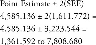
Therefore, you are 95% confident that monthly room occupancy at Stoke’s Lodge will be between 1,362 and 7,809 if the average monthly gas price is $3.65 per gallon and there are 6,800 employees working in casinos.
One Last Look at the Stoke’s Lodge Multiple Regression Model
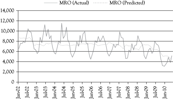
The graph in Figure 6.2 shows one final look at the Stoke’s Lodge multiple regression model evaluated in this chapter. You see that the predicted line captures the downward trend in the model. However, it does not capture the seasonality that is present in the actual data. In chapter 8, you will learn to capture seasonal variation with the use of qualitative dummy variables which will greatly improve this model.
Summary and Looking Ahead
In this chapter you have learned the difference between simple and multiple regression analysis. You have learned how to apply the five-step procedure used to evaluate a multiple regression model. First, it is necessary to determine whether the model makes logical sense. Second, you should check for statistical significance of the slope terms for all independent variables. You now know a new “p-value” method that can be used to determine statistical significance. Third, you can determine the explanatory power of the model by evaluating the adjusted coefficient of determination or adj-R2. You learned a new hypothesis test that is related to the coefficient of determination that tests the overall significance of the regression model. Next, if you have time-series data, you need to check for serial correlation. Finally, you need to check for multicollinearity between independent variables. As you read through the rest of the book you will use this procedure to evaluate multiple regression models. Specifically, in chapter 7, you will apply this five-step procedure to a market share multiple regression example. Then, in chapter 8, you will build upon your understanding of multiple regression analysis by including qualitative independent variables in the model. In chapter 10, you will see the development and evaluation of multiple regression models for sales for Abercrombie & Fitch.
What You Have Learned in Chapter 6
• To identify the five steps involved in evaluating a multiple regression model.
• To evaluate whether a multiple regression model makes logical sense.
• To check for statistical significance of all slope terms in a multiple regression model.
• To use the p-value method to evaluate statistical significance.
• To evaluate the explanatory power of a multiple regression model.
• To test the overall significance of a multiple regression model.
• To check for serial correlation in multiple regression models with time-series data.
• To check for multicollinearity in multiple regression models.
• To make a point and interval estimate based on a multiple regression model.
Appendix 6A: Critical Values of the F-distribution at a 95% Confidence Level
Source: Modified from, NIST/SEMATECH e-Handbook of Statistical
Methods, http://www.itl.nist.gov/div898/handbook/, February 6, 2012.
NOTES
1 The t-table in Appendix 4B does not provide critical values for 98 df. Therefore, you can approximate it with the value for 120 df, the closest value in the table.
2 The relationship between R2 and adj-R2 is  where n represents the number of observations and k represents the number of independent variables. If n is large relative to k there will be little difference between R2 and adj-R2.
3 Again, one would rarely calculate the adjusted coefficient of determination manually. It will generally be given in the computer printout and is most often identified as “Adjusted R Squared” or “adj-R2.”
4 This is equivalent to the null hypothesis that R2 (or adj-R2) is equal to 0.
5 This is equivalent to the alternative hypothesis that R2 (or adj-R2) is not equal to 0.
6 The denominator df of 98 is not given on the F-table in Appendix 6A. Therefore, you can approximate it using the closest value for the denominator df which in this case is 120.
7 The DW table in Appendix 4C only goes up to 40 observations. So, you can approximate with that value.
