Chapter 16
![]()
Database Workload Optimization
So far, you have learned about a number of aspects that can affect query performance, such as the tools that you can use to analyze query performance and the optimization techniques you can use to improve query performance. Next, you will learn how to apply this information to analyze, troubleshoot, and optimize the performance of a database workload. In this chapter, I cover the following topics:
- The characteristics of a database workload
- The steps involved in database workload optimization
- How to identify costly queries in the workload
- How to measure the baseline resource use and performance of costly queries
- How to analyze factors that affect the performance of costly queries
- How to apply techniques to optimize costly queries
- How to analyze the effects of query optimization on the overall workload
Workload Optimization Fundamentals
Optimizing a database workload often fits the 80/20 rule: 80 percent of the workload consumes about 20 percent of server resources. Trying to optimize the performance of the majority of the workload is usually not very productive. So, the first step in workload optimization is to find the 20 percent of the workload that consumes
80 percent of the server resources.
Optimizing the workload requires a set of tools to measure the resource consumption and response time of the different parts of the workload. As you saw in Chapter 3, SQL Server provides a set of tools and utilities to analyze the performance of a database workload and individual queries.
In addition to using these tools, it is important to know how you can use different techniques to optimize a workload. The most important aspect of workload optimization to remember is that not every optimization technique is guaranteed to work on every performance problem. Many optimization techniques are specific to certain database application designs and database environments. Therefore, for each optimization technique, you need to measure the performance of each part of the workload (that is, each individual query) before and after you apply an optimization technique. After this, you need to measure the impact of the optimization on the complete workload using the testing techniques outlined in Chapter 15.
It is not unusual to find that an optimization technique has little effect—or even a negative effect—on the other parts of the workload, thereby hurting the overall performance of the workload. For instance, a nonclustered index added to optimize a SELECT statement can hurt the performance of UPDATE statements that modify the value of the indexed column. The UPDATE statements have to update index rows in addition to the data rows. However, as demonstrated in Chapter 4, sometimes indexes can improve the performance of action queries, too. Therefore, improving the performance of a particular query could benefit or hurt the performance of the overall workload. As usual, your best course of action is to validate any assumptions through testing.
Workload Optimization Steps
The process of optimizing a database workload follows a specific series of steps. As part of this process, you will use the set of optimization techniques presented in previous chapters. Since every performance problem is a new challenge, you can use a different set of optimization techniques for troubleshooting different performance problems. Just remember that the first step is always to ensure that the server is well configured and operating within acceptable limits, as defined in Chapter 2.
To understand the query optimization process, you will simulate a sample workload using a set of queries. These are the optimization steps you will follow as you optimize the sample workload:
1. Capture the workload.
2. Analyze the workload.
3. Identify the costliest/most frequently called/longest running query.
4. Quantify the baseline resource use of the costliest query.
5. Determine the overall resource use.
6. Compile detailed information on resource use.
7. Analyze and optimize external factors.
8. Analyze the use of indexes.
9. Analyze the batch-level options used by the application.
10. Analyze the effectiveness of statistics.
11. Analyze the need for defragmentation.
12. Analyze the internal behavior of the costliest query.
13. Analyze the query execution plan.
14. Identify the costly operators in the execution plan.
15. Analyze the effectiveness of the processing strategy.
16. Optimize the costliest query.
17. Analyze the effects of the changes on database workload.
18. Iterate through multiple optimization phases.
As explained in Chapter 1, performance tuning is an iterative process. Therefore, you should iterate through the performance optimization steps multiple times until you achieve the desired application performance targets. After a certain period of time, you will need to repeat the process to address the impact on the workload caused by database changes.
Sample Workload
To troubleshoot SQL Server performance, you need to know the SQL workload that is executed on the server. You can then analyze the workload to identify causes of poor performance and applicable optimization steps. Ideally, you should capture the workload on the SQL Server facing the performance problems. In this chapter, you will use a set of queries to simulate a sample workload, so that you can follow the optimization steps listed in the previous section. The sample workload you'll use consists of a combination of good and bad queries.
![]() Note I recommend you restore a clean copy of the AdventureWorks2008R2 database, so that any artifacts left over from previous chapters are completely removed.
Note I recommend you restore a clean copy of the AdventureWorks2008R2 database, so that any artifacts left over from previous chapters are completely removed.
The very simple test workload is simulated by the following set of sample stored procedures
(workload.sql in the download); you execute these using the second script (exec.sql in the download)
on the AdventureWorks2008R2 database:
USE AdventureWorks2008R2;
GO
CREATE PROCEDURE dbo.spr_ShoppingCart
@ShoppingCartId VARCHAR(50)
AS
--provides the output from the shopping cart including the line total
SELECT sci.Quantity,
p.ListPrice,
p.ListPrice * sci.Quantity AS LineTotal,
p.[Name]
FROM Sales.ShoppingCartItem AS sci
JOIN Production.Product AS p
ON sci.ProductID = p.ProductID
WHERE sci.ShoppingCartID = @ShoppingCartId ;
GO
CREATE PROCEDURE dbo.spr_ProductBySalesOrder @SalesOrderID INT
AS
/*provides a list of products from a particular sales order,
and provides line ordering by modified date but ordered by product name*/
SELECT ROW_NUMBER() OVER (ORDER BY sod.ModifiedDate) AS LineNumber,
p.[Name],
sod.LineTotal
FROM Sales.SalesOrderHeader AS soh
JOIN Sales.SalesOrderDetail AS sod
ON soh.SalesOrderID = sod.SalesOrderID
JOIN Production.Product AS p
ON sod.ProductID = p.ProductID
WHERE soh.SalesOrderID = @SalesOrderID
ORDER BY p.[Name] ASC ;
GO
CREATE PROCEDURE dbo.spr_PersonByFirstName
@FirstName NVARCHAR(50)
AS
--gets anyone by first name from the Person table
SELECT p.BusinessEntityID,
p.Title,
p.LastName,
p.FirstName,
p.PersonType
FROM Person.Person AS p
WHERE p.FirstName = @FirstName ;
GO
CREATE PROCEDURE dbo.spr_ProductTransactionsSinceDate
@LatestDate DATETIME,
@ProductName NVARCHAR(50)
AS
--Gets the latest transaction against
-all products that have a transaction
SELECT p.Name,
th.ReferenceOrderID,
th.ReferenceOrderLineID,
th.TransactionType,
th.Quantity
FROM Production.Product AS p
JOIN Production.TransactionHistory AS th
ON p.ProductID = th.ProductID AND
th.TransactionID = (SELECT TOP (1)
th2.TransactionID
FROM Production.TransactionHistory th2
WHERE th2.ProductID = p.ProductID
ORDER BY th2.TransactionID DESC
)
WHERE th.TransactionDate > @LatestDate AND
p.Name LIKE @ProductName ;
GO
CREATE PROCEDURE dbo.spr_PurchaseOrderBySalesPersonName @LastName NVARCHAR(50)
AS
SELECT poh.PurchaseOrderID,
poh.OrderDate,
pod.LineTotal,
p.[Name] AS ProductName,
e.JobTitle,
per.LastName + ', ' + per.FirstName AS SalesPerson
FROM Purchasing.PurchaseOrderHeader AS poh
JOIN Purchasing.PurchaseOrderDetail AS pod
ON poh.PurchaseOrderID = pod.PurchaseOrderID
JOIN Production.Product AS p
ON pod.ProductID = p.ProductID
JOIN HumanResources.Employee AS e
ON poh.EmployeeID = e.BusinessEntityID
JOIN Person.Person AS per
ON e.BusinessEntityID = per.BusinessEntityID
WHERE per.LastName LIKE @LastName
ORDER BY per.LastName,
per.FirstName ;
GO
Once these procedures are created, you can execute them using the following scripts:
EXEC dbo.spr_ShoppingCart
'20621' ;
GO
EXEC dbo.spr_ProductBySalesOrder
43867 ;
GO
EXEC dbo.spr_PersonByFirstName
'Gretchen' ;
GO
EXEC dbo.spr_ProductTransactionsSinceDate
@LatestDate = '9/1/2004',
@ProductName = 'Hex Nut%' ;
GO
EXEC dbo.spr_PurchaseOrderBySalesPersonName
@LastName = 'Hill%' ;
GO
This is an extremely simplistic workload that's here just to illustrate the process. You're going to see hundreds and thousands of additional calls in a typical system. As simple as it is, however, this sample workload does consist of the different types of queries you usually execute on SQL Server:
- Queries using aggregate functions
- Point queries that retrieve only one row or a small number of rows; usually, these are the best kind for performance
- Queries joining multiple tables
- Queries retrieving a narrow range of rows
- Queries performing additional result set processing, such as providing a sorted output
The first optimization step is to identify the worst performing queries, as explained in the next section.
Capturing the Workload
As a part of the diagnostic-data collection step, you must define an extended event session to capture the workload on the database server. You can use the tools and methods recommended in Chapter 3 to do this.
Table 16-1 lists the specific events that you should use to measure how resource intensive the queries are.
Table 16-1. Events to Capture Information About Costly Queries
|
Category |
Event |
|
Execution |
rpc_completed sql_batch_completed |
As explained in Chapter 3, for production databases it is recommended that you capture the output of the Extended Events session to a file. Here are a couple significant advantages to capturing output to a file:
- Since you intend to analyze the SQL queries once the workload is captured, you do not need to display the SQL queries while capturing them.
- Running the Session through SSMS doesn't provide a very flexible timing control over the tracing process.
Let's look at timing control more closely. Assume you want to start capturing events at 11 p.m. and record the SQL workload for 24 hours. You can define an extended event session using the GUI or through TSQL. However, you don't have to start the process until you're ready. This means you can create commands in SQL Agent or with some other scheduling tool to start and stop the process with the ALTER EVENT SESSION command:
ALTER EVENT SESSION <sessionname>
ON SERVER
STATE = <start/stop> ;
For this example, I've put a filter on the session to capture events only from the AdventureWorks2008R2 database. The file will only capture queries against that database, reducing the amount of information I need to deal with. This may be a good choice for your systems, too.
Analyzing the Workload
Once the workload is captured in a file, you can analyze the workload either by browsing through the data using SSMS or by importing the content of the output file into a database table.
SSMS provides the following two methods for analyzing the content of the file, both of which are relatively straightforward:
- Sort the output on a data column by right-clicking to select a sort order or to Group By a particular column: You may want to select columns from the Details tab and use the Show column in table command to move them up. Once there, you can issue grouping and sorting commands on that column.
- Rearrange the output to a selective list of columns and events: You can change the output displayed through SSMS by right-clicking the table and selecting Pick Columns from the context menu. This lets you do more than simply pick and choose columns; it also lets you combine them into new columns.
Unfortunately, using SSMS provides limited ways of analyzing the Extended Events output. For instance, consider a query that is executed frequently. Instead of looking at the cost of only the individual execution of the query, you should also try to determine the cumulative cost of repeatedly executing the query within a fixed period of time. Although the individual execution of the query may not be that costly, the query may be executed so many times that even a little optimization may make a big difference. SSMS is not powerful enough to
help analyze the workload in such advanced ways. So, while you can group by the batch_text column, the differences in parameter values mean that you'll see different groupings of the same stored procedure call.
For in-depth analysis of the workload, you must import the content of the trace file into a database table. The output from the session puts most of the important data into an XML field, so you'll want to query it as you
load the data as follows:
IF (SELECT OBJECT_ID('dbo.ExEvents')
) IS NOT NULL
DROP TABLE dbo.ExEvents ;
GO
WITH xEvents
AS (SELECT object_name AS xEventName,
CAST (event_data AS xml) AS xEventData
FROM sys.fn_xe_file_target_read_
file('D:ApathQuery Performance Tuning*.xel',
NULL, NULL, NULL)
)
SELECT xEventName,
xEventData.value('(/event/data[@name=''duration'']/value)[1]',
'bigint') Duration,
xEventData.value('(/event/data[@name=''physical_reads'']/value)[1]',
'bigint') PhysicalReads,
xEventData.value('(/event/data[@name=''logical_reads'']/value)[1]',
'bigint') LogicalReads,
xEventData.value('(/event/data[@name=''cpu_time'']/value)[1]',
'bigint') CpuTime,
CASE xEventName
WHEN 'sql_batch_completed'
THEN
xEventData.value('(/event/data[@name=''batch_text'']/value)[1]',
'varchar(max)')
WHEN 'rpc_completed'
THEN
xEventData.value('(/event/data[@name=''statement'']/value)[1]',
'varchar(max)')
END AS SQLText,
xEventData.value('(/event/data[@name=''query_plan_hash'']/value)[1]',
'binary(8)') QueryPlanHash
INTO dbo.ExEvents
FROM xEvents ;
You need to substitute your own path and file name for <ExEventsFileName>. Once you have the content in a table, you can use SQL queries to analyze the workload. For example, to find the slowest queries, you can execute this SQL query:
SELECT *
FROM dbo.ExEvents AS ee
ORDER BY ee.Duration DESC ;
The preceding query will show the single costliest query, and it is adequate for the tests you're running in this chapter. You may also want to run a query like this on a production system; however, it's more likely you'll want to work off of aggregations of data, as in this example:
SELECT ee.BatchText,
SUM(Duration) AS SumDuration,
AVG(Duration) AS AvgDuration,
COUNT(Duration) AS CountDuration
FROM dbo.ExEvents AS ee
GROUP BY ee.BatchText ;
Executing this query lets you order things by the fields you're most interested in—say, CountDuration to get the most frequently called procedure or SumDuration to get the procedure that runs for the longest cumulative amount of time. You need a method to remove or replace parameters and parameter values. This is necessary in order to aggregate based on just the procedure name or just the text of the query without the parameters or parameter values (since these will be constantly changing). The objective of analyzing the workload is to identify the costliest query (or costly queries in general); the next section covers how to do this.
Identifying the Costliest Query
As just explained, you can use SSMS or the query technique to identify costly queries for different criteria. The queries in the workload can be sorted on the CPU, Reads, or Writes column to identify the costliest query, as discussed in Chapter 3. You can also use aggregate functions to arrive at the cumulative cost, as well as individual costs. In a production system, knowing the procedure that is accumulating the longest run times, the most CPU usage, or the largest number of reads and writes is frequently more useful than simply identifying the query that had the highest numbers one time.
Since the total number of reads usually outnumbers the total number of writes by at least seven to eight times for even the heaviest OLTP database, sorting the queries on the Reads column usually identifies more bad queries than sorting on the Writes column (but you should always test this on your systems). It's also worth looking at the queries that simply take the longest to execute. As outlined in Chapter 3, you can capture wait states with Performance Monitor and view those along with a given query to help identify why a particular query is taking a long time to run. Each system is different. In general, I approach the most frequently called procedures first; then the longest-running; and finally, those with the most reads. Of course, performance tuning is an iterative process, so you will need to reexamine each category on a regular basis.
To analyze the sample workload for the worst-performing queries, you need to know how costly the queries are in terms of duration or reads. Since these values are known only after the query completes its execution, you are mainly interested in the completed events. (The rationale behind using completed events for performance analysis is explained in detail in Chapter 3.)
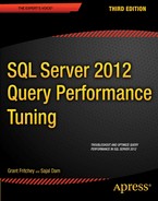
For presentation purposes, open the trace file in SSMS. Figure 16-1 shows the captured trace output after moving several columns to the grid.
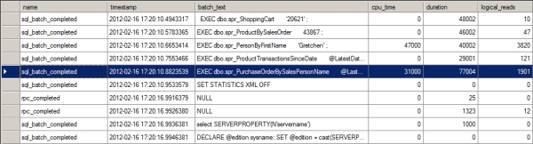
Figure 16-1. Extended Events session output showing the SQL workload
The worst-performing query in terms of duration is also one of the worst in terms of CPU usage as well as reads. That procedure, spr_PurchaseOrderByhSalesPersonName, is highlighted in Figure 16-1 (you may have different values, but this query is likely to be the worst-performing query or at least one of the worst). The query inside that procedure is presented here for easy reference:
SELECT poh.PurchaseOrderID,
poh.OrderDate,
pod.LineTotal,
p.[Name] AS ProductName,
e.JobTitle,
per.LastName + ', ' + per.FirstName AS SalesPerson
FROM Purchasing.PurchaseOrderHeader AS poh
JOIN Purchasing.PurchaseOrderDetail AS pod
ON poh.PurchaseOrderID = pod.PurchaseOrderID
JOIN Production.Product AS p
ON pod.ProductID = p.ProductID
JOIN HumanResources.Employee AS e
ON poh.EmployeeID = e.BusinessEntityID
JOIN Person.Person AS per
ON e.BusinessEntityID = per.BusinessEntityID
WHERE per.LastName LIKE @LastName
ORDER BY per.LastName,
per.FirstName ;
Another method open to you if you can't run Extended Events is to use the sys.dm_exec_query_stats DMO. This will provide you with aggregate information about all the queries currently in cache. It's a fast way to identify the most frequently called, longest running, and most resource intensive procedures. It brings along the added benefit of being able to quickly join to other DMOs to pull out the execution plan and other interesting information.
Once you've identified the worst-performing query, the next optimization step is to determine the resources consumed by the query.
Determining the Baseline Resource Use of the Costliest Query
The current resource use of the worst-performing query can be considered as a baseline figure before you apply any optimization techniques. You may apply different optimization techniques to the query, and you can compare the resultant resource use of the query with the baseline figure to determine the effectiveness of a given optimization technique. The resource use of a query can be presented in two categories:
- Overall resource use
- Detailed resource use
The overall resource use of the query provides a gross figure for the amount of hardware resources consumed
by the worst performing query. You can compare the resource use of an optimized query to the overall resource use of a nonoptimized query to ensure the overall effectiveness of the performance techniques you've
applied.
You can determine the overall resource use of the query from the workload trace. Table 16-3 shows the overall use of the query from the trace in Figure 16-1.
Table 16-3. Data Columns Representing the Amount of Resources Used by a Query
|
Data Column |
Value |
Description |
|
LogicalReads |
1901 |
Number of logical reads performed by the query. If a page is not found in memory, then a logical read for the page will require a physical read from the disk to fetch the page to the memory first. |
|
Writes |
0 |
Number of pages modified by the query. |
|
CPU |
31 ms |
How long the CPU was used by the query. |
|
Duration |
77 ms |
The time it took SQL Server to process this query from compilation to returning the result set. |
![]() Note In your environment, you may have different figures for the preceding data columns. Irrespective of the data columns' absolute values, it's important to keep track of these values, so that you can compare them with the corresponding values later.
Note In your environment, you may have different figures for the preceding data columns. Irrespective of the data columns' absolute values, it's important to keep track of these values, so that you can compare them with the corresponding values later.
You can break down the overall resource use of the query to locate bottlenecks on the different database tables accessed by the query. This detailed resource use helps you determine which table accesses are the most problematic. Understanding the wait states in your system will help you identify where you need to focus your tuning, whether it's on CPU usage, reads, or writes. A rough rule of thumb can be to simply look at duration; however, duration can be affected by so many factors that it's an imperfect measure, at best. In this case, I'll spend time on all three: CPU usage, reads, and duration. Reads are a popular measure of performance, but they can be as problematic to look at in isolation as duration. This is why I spend time on all the values.
As you saw in Chapter 3, you can obtain the number of reads performed on the individual tables accessed by a given query from the STATISTICS IO output for that query. You can also set the STATISTICS TIME option to get the basic execution time and CPU time for the query, including its compile time. You can obtain this output by reexecuting the query with the SET statements as follows (or by selecting the Set Statistics IO checkbox in the query window):
DBCC FREEPROCCACHE() ;
DBCC DROPCLEANBUFFERS ;
GO
SET STATISTICS TIME ON ;
GO
SET STATISTICS IO ON ;
GO
EXEC dbo.spr_PurchaseOrderBySalesPersonName
@LastName = 'Hill%' ;
GO
SET STATISTICS TIME OFF ;
GO
SET STATISTICS IO OFF ;
GO
To simulate the same first-time run shown in Figure 16-1, clean out the data stored in memory using DBCC DROPCLEANBUFFERS (not to be run on a production system) and remove the procedure from cache by running DBCC FREEPROCCACHE (also not to be run on a production system).
The STATISTICS output for the worst performing query looks like this:
SQL Server parse and compile time:
CPU time = 0 ms, elapsed time = 1 ms.
DBCC execution completed. If DBCC printed error messages, contact your system administrator.
SQL Server Execution Times:
CPU time = 0 ms, elapsed time = 1 ms.
DBCC execution completed. If DBCC printed error messages, contact your system administrator.
SQL Server Execution Times:
CPU time = 0 ms, elapsed time = 2 ms.
SQL Server parse and compile time:
CPU time = 0 ms, elapsed time = 1 ms.
SQL Server Execution Times:
CPU time = 0 ms, elapsed time = 0 ms.
SQL Server parse and compile time:
CPU time = 0 ms, elapsed time = 0 ms.
SQL Server Execution Times:
CPU time = 0 ms, elapsed time = 0 ms.
SQL Server parse and compile time:
CPU time = 0 ms, elapsed time = 0 ms.
SQL Server parse and compile time:
CPU time = 46 ms, elapsed time = 109 ms.
(1496 row(s) affected)
Table 'Worktable'. Scan count 0, logical reads 0, physical reads 0, read-ahead reads 0,
lob logical reads 0, lob physical reads 0, lob read-ahead reads 0.
Table 'PurchaseOrderDetail'. Scan count 1, logical reads 66, physical reads 1,
read-ahead reads 64, lob logical reads 0, lob physical reads 0, lob read-ahead reads 0.
Table 'PurchaseOrderHeader'. Scan count 4, logical reads 1673, physical reads 8,
read-ahead reads 8, lob logical reads 0, lob physical reads 0, lob read-ahead reads 0.
Table 'Employee'. Scan count 0, logical reads 174, physical reads 2, read-ahead reads 0,
lob logical reads 0, lob physical reads 0, lob read-ahead reads 0.
Table 'Person'. Scan count 1, logical reads 4, physical reads 1, read-ahead reads 2,
lob logical reads 0, lob physical reads 0, lob read-ahead reads 0.
Table 'Product'. Scan count 1, logical reads 5, physical reads 1, read-ahead reads 8,
lob logical reads 0, lob physical reads 0, lob read-ahead reads 0.
SQL Server Execution Times:
CPU time = 16 ms, elapsed time = 435 ms.
SQL Server Execution Times:
CPU time = 62 ms, elapsed time = 544 ms.
Table 16-4 summarizes the output of STATISTICS IO.
Table 16-4. Breaking Down the Output from STATISTICS IO
|
Table |
Logical Reads |
|
Purchasing.PurchaseOrderDetail |
66 |
|
Purchasing.PurchaseOrderHeader |
1,673 |
|
Person.Employee |
174 |
|
Person.Person |
4 |
|
Production.Product |
5 |
Usually, the sum of the reads from the individual tables referred to in a query will be less than the total number of reads performed by the query. This is because additional pages have to be read to access internal database objects, such as sysobjects, syscolumns, and sysindexes.
Table 16-5 summarizes the output of STATISTICS TIME.
Table 16-5. Breaking down the Output from STATISTICS TIME
|
Event |
Duration |
CPU |
|
Compile |
109 ms |
46 ms |
|
Execution |
435 ms |
16 ms |
|
Completion |
544 ms |
62 ms |
Don't use the logical reads in isolation from the execution times. You need to take all the measures into account when determining poorly performing queries. Conversely, don't assume that the execution time is a perfect measure, either. Resource contention plays a big part in execution time, so you'll see some variation in this measure. Use both values, but use them with a full understanding of what they mean.
Once the worst performing query has been identified and its resource use has been measured, the next optimization step is to determine the factors that are affecting the performance of the query. However, before you do this, you should check to see whether any factors external to the query might be causing that poor performance.
Analyzing and Optimizing External Factors
In addition to factors such as query design and indexing, external factors can affect query performance. Thus, before diving into the execution plan of the query, you should analyze and optimize the major external factors that can affect query performance. Here are some of those external factors:
- The connection options used by the application
- The statistics of the database objects accessed by the query
- The fragmentation of the database objects accessed by the query
Analyzing the Connection Options Used by the Application
When making a connection to SQL Server, various options, such as ANSI_NULL or CONCAT_NULL_YIELDS_NULL, can be set differently than the defaults for the server or the database. However, changing these settings per connection can lead to recompiles of stored procedures, causing slower behavior. Also, some options, such as ARITHABORT, must be set to ON when dealing with indexed views and certain other specialized indexes. If they are not, you can get poor performance or even errors in the code. For example, setting ANSI_WARNINGS to OFF will cause the optimizer to ignore indexed views and indexed computed columns when generating the execution plan. You can use the output from Extended Events to see this information. The options_text column contains the settings used by the connection in the login event and in the existing_connection event, as shown in Figure 16-2.
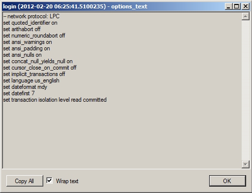
Figure 16-2. An existing connection showing the batch-level options
This column does more than display the batch-level options; it also lets you check the transaction isolation level. You can also get these settings from the properties of the first operator in an execution plan.
I recommend using the ANSI standard settings, in which you set the following options to ON: ANSI_NULLS, ANSI_NULL_DFLT_ON, ANSI_PADDING, ANSI_WARNINGS, CURS0R_CL0SE_0N_C0MMIT, IMPLICIT_TRANSACTIONS, and QUOTED_IDENTIFIER. You can use the single command SET ANSIDEFAULTS ON to set them all to ON at the same time.
Analyzing the Effectiveness of Statistics
The statistics of the database objects referred to in the query are one of the key pieces of information that the query optimizer uses to decide upon certain execution plans. As explained in Chapter 7, the optimizer generates the execution plan for a query based on the statistics of the objects referred to in the query. The optimizer looks at the statistics of the database objects referred to in the query and estimates the number of rows affected. In this way, it determines the processing strategy for the query. If a database object's statistics are not accurate, then the optimizer may generate an inefficient execution plan for the query.
As explained in Chapter 7, you can check the statistics of a table and its indexes using DBCC SHOW_STATISTICS. There are five tables referenced in this query: Purchasing.PurchaseOrderHeader, Purchasing.PurchaseOrderDetail, Person.Employee, Person.Person, and Production.Product. You must know
which indexes are in use by the query to get the statistics information about them. You can determine this when you look at the execution plan. For now, I'll check the statistics on the primary key of the Purchasing.PurchaseOrderHeader table since it had the most reads, as shown in Table 16-4. Now run the following
query:
DBCC SHOW_STATISTICS('Purchasing.PurchaseOrderHeader',
'PK_PurchaseOrderHeader_PurchaseOrderID') ;
When the preceding query completes, you'll see the output shown in Figure 16-3.
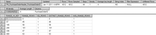
Figure 16-3. SHOW_STATISTICS output for Purchasing.PurchaseOrderHeader
You can see the selectivity on the index is very high since the density is quite low, as shown in the All density column. In this instance, it's doubtful that statistics are likely to be the cause of this query's poor performance. You can also check the Updated column to determine the last time this set of statistics was updated. If has been more than a few days since the statistics were updated, then you need to check your statistics maintenance plan, and you should update these statistics manually.
Analyzing the Need for Defragmentation
As explained in Chapter 8, a fragmented table increases the number of pages to be accessed by a query, which adversely affects performance. For this reason, you should ensure that the database objects referred to in the query are not too fragmented.
You can determine the fragmentation of the five tables accessed by the worst performing query by running a query against sys.dm_db_index_physical_stats (--showcontig in the download). Begin by running the query against the Purchasing.PurchaseOrderHeader table:
SELECT s.avg_fragmentation_in_percent,
s.fragment_count,
s.page_count,
s.avg_page_space_used_in_percent,
s.record_count,
s.avg_record_size_in_bytes,
s.index_id
FROM sys.dm_db_index_physical_stats(DB_ID('AdventureWorks2008R2'),
OBJECT_ID(N'Purchasing.PurchaseOrderHeader'),
NULL, NULL, 'Sampled') AS s
WHERE s.record_count > 0
ORDER BY s.index_id ;
Figure 16-4 shows the output of this query.

Figure 16-4. The index fragmentation of the Purchasing.PurchaseOrderHeader table
If you run the same query for the other four tables (in order: Purchasing.PurchaseOrderDetail, Production.Product, Person.Employee, and Person.Person), the output will look like Figure 16-5.
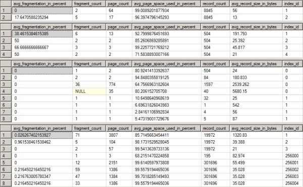
Figure 16-5. The index fragmentation for the four tables in the problem query
The fragmentation of the Purchasing.PurchaseOrderHeader table is extremely light: 33 percent. Meanwhile, the avg_page_space_used_in_percent is greater than 90 percent for all the indexes. When you take into account the number of pages for the indexes on the table—three or less—you're very unlikely to get an improvement in performance by defragging the index (assuming you can), as detailed in Chapter 8.
The same can be said of Purchasing.PurchaseOrderDetail, which has very low fragmentation and a low page count. Production.Product has slightly higher degrees of fragmentation; but again, the page count is very low, so defragging the index is not likely to help much. Person.Employee has one index with 66 percent fragmentation; once again, however, it's only on three pages. Finally, Person.Person has almost no fragmentation to speak of.
Here's an experiment to try as part of the iterative performance-tuning process. Run the index defragmentation script supplied in Chapter 8 (and repeated here):
DECLARE @DBName NVARCHAR(255),
@TableName NVARCHAR(255),
@SchemaName NVARCHAR(255),
@IndexName NVARCHAR(255),
@PctFrag DECIMAL,
@Defrag NVARCHAR(MAX)
IF EXISTS ( SELECT *
FROM sys.objects
WHERE OBJECT_ID = OBJECT_ID(N'#Frag') )
DROP TABLE #Frag
CREATE TABLE #Frag (
DBName NVARCHAR(255),
TableName NVARCHAR(255),
SchemaName NVARCHAR(255),
IndexName NVARCHAR(255),
AvgFragment DECIMAL
)
EXEC sys.sp_MSforeachdb
'INSERT INTO #Frag ( DBName,
TableName, SchemaName,
IndexName,
AvgFragment )
SELECT ''?'' AS DBName,
t.Name AS TableName,
sc.Name AS SchemaName,
i.name ASIndexName,
s.avg_fragmentation_in_percent
FROM ?.sys.dm_db_index_physical_stats(DB_ID(''?''),
NULL, NULL, NULL,
''Sampled'') AS s JOIN ?.sys.indexes i
ON s.Object_Id = i.Object_id
AND s.Index_id = i.Index_id
JOIN ?.sys.tables t
ON i.Object_id = t.Object_Id
JOIN ?.sys.schemas sc
ON t.schema_id = sc.SCHEMA_ID
WHERE s.avg_fragmentation_in_percent > 20
AND t.TYPE = ''U''
AND s.page_count > 8
ORDER BY TableName,IndexName';
DECLARE cList CURSOR
FOR
SELECT *
FROM #Frag;
OPEN cList;
FETCH NEXT FROM cList
INTO @DBName, @TableName, @SchemaName, @IndexName, @PctFrag;
WHILE FETCH_STATUS = 0
BEGIN
IF @PctFrag BETWEEN 20.0 AND 40.0
BEGIN
SET @Defrag = N'ALTER INDEX ' + @IndexName + ' ON ' + @DBName +
'.' + @SchemaName + '.' + @TableName + ' REORGANIZE';
EXEC sp_executesql
@Defrag;
PRINT 'Reorganize index: ' + @DBName + '.' + @SchemaName + '.' +
@TableName + '.' + @IndexName;
END
ELSE
IF @PctFrag > 40.0
BEGIN
SET @Defrag = N'ALTER INDEX ' + @IndexName + ' ON ' +
@DBName + '.' + @SchemaName + '.' + @TableName +
' REBUILD';
EXEC sp_executesql
@Defrag;
PRINT 'Rebuild index: ' + @DBName + '.' + @SchemaName +
'.' + @TableName + '.' + @IndexName;
END
FETCH NEXT FROM cList
INTO @DBName, @TableName, @SchemaName, @IndexName, @PctFrag;
END
CLOSE cList;
DEALLOCATE cList;
DROP TABLE #Frag;
After defragging the indexes on the database, rerun the query against sys.dm_db_index_ physicalstats for all five tables. This will let you determine the changes in the index defragmentation, if any (see Figure 16-6).
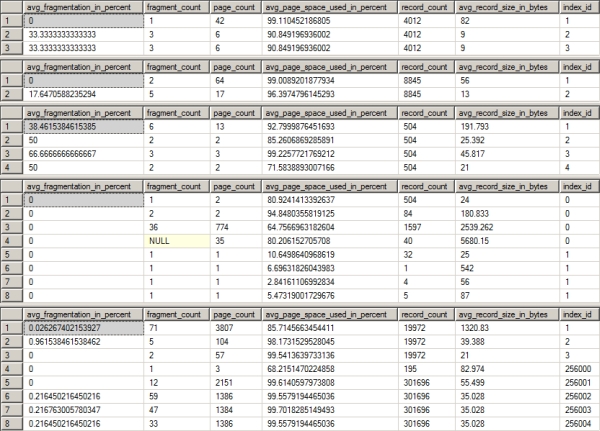
Figure 16-6. The index fragmentation of Production.Product after rebuilding indexes
As you can see in Figure 16-6, the fragmentation was not reduced at all in any of the indexes in the tables used by the poorest performing query.
Once you've analyzed the external factors that can affect the performance of a query and resolved the nonoptimal ones, you should analyze internal factors, such as improper indexing and query design.
Analyzing the Internal Behavior of the Costliest Query
Now that the statistics are up-to-date, you can analyze the processing strategy for the query chosen by the optimizer to determine the internal factors affecting the query's performance. Analyzing the internal factors that can affect query performance involves these steps:
- Analyzing the query execution plan
- Identifying the costly steps in the execution plan
- Analyzing the effectiveness of the processing strategy
Analyzing the Query Execution Plan
To see the execution plan, click the Show Actual Execution Plan button to enable it, and then run stored procedure. Be sure you're doing these types of tests on a non-production system. For more details on reading execution plans, check out my book, SQL Server Execution Plans (Simple Talk Publishing, 2008). Figure 16-7 shows the graphical execution plan of the worst performing query.
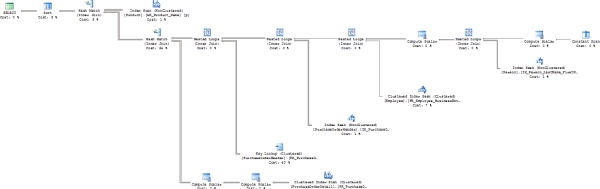
Figure 16-7. The graphical execution plan of the worst performing query
You can observe the following from this execution plan, as explained in Chapter 3:
- SELECT properties:
- Optimization Level: Full
- Reason for Early Termination: Timeout
- Data access:
- Index scan on nonclustered index, Product.AK_Product_Name
- Index seek on nonclustered index, Person.IX_Person_LastName_FirstName_MiddleName
- Index seek on clustered index, Employee.PK_Employee_BusinessEntityID
- Index seek on nonclustered index, PurchaseOrderHeader.IX_PurchaseOrderHeader_EmployeelD
- Key lookup on PurchaseOrderHeader.PK_PurchaseOrderHeader_PurchaseOrderID
- Index scan on clustered index, PurchaseOrderDetail.PK_PurchaseOrderDetail_PurchaseOrderDetaillD
- Join strategy:
- Nested loop join between the constant scan and Person.Person table with the Person.Person table as the outer table
- Nested loop join between the Person.Person table and Person.Employee with the Person.Employee table as the outer table
- Nested loop join between the Person.Person table and the Purchasing.PurchaseOrderHeader table that was also the outer table
- Nested loop join between the Purchasing.PurchaseOrderHeader index and the Purchasing.PurchaseOrderHeader primary key with the primary key as the outer table
- Hash match join between the Purchasing.PurchaseOrderHeader table and the Purchasing.PurchaseOrderDetail table with Purchasing.PurchaseOrderDetail as the outer table
- Hash match join between the Production.Product and Purchasing.PurchaseOrderDetail tables with the Purchasing.PurchaseOrderDetail table as the outer table
- Additional processing:
- Constant scan to provide a placeholder for the @LastName variable's LIKE operation
- Compute scalar that defined the constructs of the @LastName variable's LIKE operation, showing the top and bottom of the range and the value to be checked
- Compute scalar that combines the FirstName and LastName columns into a new column
- Compute scalar that calculates the LineTotal column from the Purchasing.PurchaseOrderDetail table
- Compute scalar that takes the calculated LineTotal and stores it as a permanent value in the result set for further processing
- Sort on the FirstName and LastName from the Person.Person table
Identifying the Costly Steps in the Execution Plan
Once you understand the execution plan of the query, the next step is to identify the steps estimated as the most costly in the execution plan. Although these costs are estimated and can be inaccurate at times, the optimization of the costly steps usually benefits the query performance the most. You can see that the following are the two costliest steps:
- Costly step 1: The key lookup on the Purchasing.PurchaseOrderHeader table is 40 percent
- Costly step 2: The hash match between Purchasing.PurchaseOrderHeader and Purchasing.PurchaseOrderDetail is 20 percent
The next optimization step is to analyze the costliest steps, so you can determine whether these steps can be optimized through techniques such as redesigning the query or indexes.
Analyzing the Processing Strategy
Since the optimization timed out, analyzing the effectiveness of the processing strategy is of questionable utility. However, you can begin evaluating it by following the traditional steps. If we're still getting a timeout after tuning the query and the structure, however, then more tuning and optimization work may be required.
Costly step 1 is a very straightforward key lookup (bookmark lookup). This problem has a number of possible solutions, many of which were outlined in Chapter 5.
Costly step 2 is the hash match between Purchasing.PurchaseOrderHeader and Purchasing.PurchaseOrderDetail. Figure 16-8 shows the number of rows coming from each of the two tables in the order listed. These represent the inner and outer portions of the hash join. As you can see, there are 763 rows coming from Purchasing.PurchaseOrderDetail and 8,845 from Purchasing.PurchaseOrderDetail. Based on these values, it's likely that the hash join is the optimal method for putting the data together. While it is possible to change this through index tuning or query hints, it's unlikely that it will help the query to do so.

Figure 16-8. Row counts leading into hash match join
![]() Tip At times you may find that no improvements can be made to the costliest step in a processing strategy. In that case, concentrate on the next costliest step to identify the problem. If none of the steps can be optimized further, then move on to the next costliest query in the workload. You may need to consider changing the database design or the construction of the query.
Tip At times you may find that no improvements can be made to the costliest step in a processing strategy. In that case, concentrate on the next costliest step to identify the problem. If none of the steps can be optimized further, then move on to the next costliest query in the workload. You may need to consider changing the database design or the construction of the query.
Optimizing the Costliest Query
Once you've diagnosed the queries with costly steps, the next stage is to implement the necessary corrections to reduce the cost of these steps.
The corrective actions for a problematic step can have one or more alternative solutions. For example, should you create a new index or structure the query differently? In such cases, you should prioritize the solutions based on their expected effectiveness and the amount of work required. For example, if a narrow index can more or less do the job, then it is usually better to prioritize that over changes to code that might lead to business testing. Making changes to code can also be the less intrusive approach. You need to evaluate each situation within the business and application construct you have.
Apply the solutions individually in the order of their expected benefit, and measure their individual effect on the query performance. Finally, you can apply the solution that provides the greatest performance improvement to correct the problematic step. Sometimes, it may be evident that the best solution will hurt other queries in the workload. For example, a new index on a large number of columns can hurt the performance of action queries. However, since that's not always true, it's better to determine the effect of such optimization techniques on the complete workload through testing. If a particular solution hurts the overall performance of the workload, choose the next best solution while keeping an eye on the overall performance of the workload.
It seems obvious from looking at the processing strategy that changing the nonclustered index on Purchasing.PurchaseOrderHeader will eliminate the key lookup. Since the output list of the key lookup includes only one relatively small column, this can be added to the IX_ PurchaseOrderHeader_EmployeeID index as an included column (--Alterlndex in the download):
CREATE NONCLUSTERED INDEX [IX_PurchaseOrderHeader_EmployeeID]
ON [Purchasing].[PurchaseOrderHeader] ([EmployeeID] ASC)
INCLUDE (OrderDate)
WITH (
DROP_EXISTING = ON) ON [PRIMARY] ;
GO
Now run the costly query again using the Test.sql script that includes the cleanup steps, as well as the statistics information. The output looks like this:
SQL Server parse and compile time:
CPU time = 0 ms, elapsed time = 0 ms.
SQL Server Execution Times:
CPU time = 0 ms, elapsed time = 0 ms.
SQL Server parse and compile time:
CPU time = 0 ms, elapsed time = 14 ms.
DBCC execution completed. If DBCC printed error messages, contact your system administrator.
SQL Server Execution Times:
CPU time = 62 ms, elapsed time = 382 ms.
DBCC execution completed. If DBCC printed error messages, contact your system administrator.
SQL Server Execution Times:
CPU time = 141 ms, elapsed time = 157 ms.
SQL Server parse and compile time:
CPU time = 0 ms, elapsed time = 0 ms.
SQL Server parse and compile time:
CPU time = 31 ms, elapsed time = 51 ms.
(1496 row(s) affected)
Table 'Worktable'. Scan count 0, logical reads 0, physical reads 0, read-ahead reads 0, lob logical reads 0, lob physical reads 0, lob read-ahead reads 0.
Table 'PurchaseOrderDetail'. Scan count 1, logical reads 66, physical reads 1,
read-ahead reads 64, lob logical reads 0, lob physical reads 0, lob read-ahead reads 0.
Table 'PurchaseOrderHeader'. Scan count 4, logical reads 11, physical reads 3,
read-ahead reads 0, lob logical reads 0, lob physical reads 0, lob read-ahead reads 0.
Table 'Employee'. Scan count 0, logical reads 174, physical reads 2, read-ahead reads 0, lob logical reads 0, lob physical reads 0, lob read-ahead reads 0.
Table 'Person'. Scan count 1, logical reads 4, physical reads 1, read-ahead reads 2, lob logical reads 0, lob physical reads 0, lob read-ahead reads 0.
Table 'Product'. Scan count 1, logical reads 5, physical reads 1, read-ahead reads 8,
lob logical reads 0, lob physical reads 0, lob read-ahead reads 0.
(1 row(s) affected)
SQL Server Execution Times:
CPU time = 16 ms, elapsed time = 196 ms.
SQL Server Execution Times:
CPU time = 47 ms, elapsed time = 247 ms.
SQL Server parse and compile time:
CPU time = 0 ms, elapsed time = 0 ms.
SQL Server Execution Times:
CPU time = 0 ms, elapsed time = 0 ms.
The number of reads on the Purchasing.PurchaseOrderTable table has dropped from 1,673 to 11. That's great! The execution time has dropped as well, but there is more you can do, and logical reads alone won't give you all the information you need. This means more tuning of the query is necessary. Figure 16-9 shows the new execution plan.
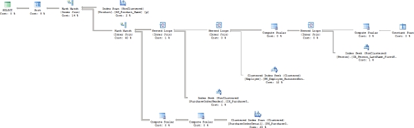
Figure 16-9. The graphical execution plan of the query after changing the nonclustered index
The key lookup is completely gone, and the query is just a bit simpler and easier to read. The estimated costs on the various operations have shifted, and the hash match join is now the costliest operation. The second costliest operation is now the clustered index scan against Purchasing.PurchaseOrderDetail. Also, the properties still show a timeout on the SELECT operator.
Analyzing the Application of a Join Hint
Since the costliest operation is now the hash join, it might make sense to try to change that to a different join. Based on the data being moved (see Figure 16-8), it's likely that the hash match was the appropriate choice. However, to see whether forcing the join to use a LOOP or MERGE might make a performance improvement, you simply need to modify the procedure:
ALTER PROCEDURE dbo.spr_PurchaseOrderBySalesPersonName
@LastName NVARCHAR(50)
AS
SELECT poh.PurchaseOrderID,
poh.OrderDate,
pod.LineTotal,
p.[Name] AS ProductName,
e.JobTitle,
per.LastName + ', ' + per.FirstName AS Salesperson
FROM Purchasing.PurchaseOrderHeader AS poh
INNER LOOP JOIN Purchasing.PurchaseOrderDetail AS pod
ON poh.PurchaseOrderID = pod.PurchaseOrderID
JOIN Production.Product AS p
ON pod.ProductID = p.ProductID
JOIN HumanResources.Employee AS e
ON poh.EmployeeID = e.BusinessEntityID
JOIN Person.Person AS per
ON e.BusinessEntityID = per.BusinessEntityID
WHERE per.LastName LIKE @LastName
ORDER BY per.LastName,
per.FirstName;
Figure 16-10 shows the resultant execution plan for the worst performing query.

Figure 16-10. A graphical execution plan of the query with a join hint
The execution plan changed radically in this iteration. The nested loop allows for a Clustered Index Seek against the Purchasing.PurchaseOrderDetail table. With the elimination of the hash match, you might think that the performance improved. Unfortunately, looking at the statistics reveals that the number of scans and reads on Purchasing.PurchaseOrderDetail increased dramatically. The scans increased to support the loop part of the Nested Loop operation, and the reads shot through the roof, from 66 to 8,960. Performance time almost doubled to 282 ms.
This is clearly not working; however, what if you changed the procedure to a merge join? There are two hash match joins this time, so you will want to eliminate both:
ALTER PROCEDURE [dbo].[spr_PurchaseOrderBySalesPersonName]
@LastName NVARCHAR(50)
AS
SELECT poh.PurchaseOrderID,
poh.OrderDate,
pod.LineTotal,
p.[Name] AS ProductName,
e.JobTitle,
per.LastName + ', ' + per.FirstName AS Salesperson
FROM Purchasing.PurchaseOrderHeader AS poh
INNER MERGE JOIN Purchasing.PurchaseOrderDetail AS pod
ON poh.PurchaseOrderID = pod.PurchaseOrderID
INNER MERGE JOIN Production.Product AS p
ON pod.ProductID = p.ProductID
JOIN HumanResources.Employee AS e
ON poh.EmployeeID = e.BusinessEntityID
JOIN Person.Person AS per
ON e.BusinessEntityID = per.BusinessEntityID
WHERE per.LastName LIKE @LastName
ORDER BY per.LastName,
per.FirstName ;
Figure 16-11 shows the execution plan that results from this new query.
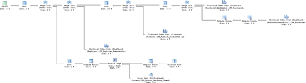
Figure 16-11. An execution plan that forces merge joins in place of the hash joins
The performance is much worse in this iteration, and you can see why. In addition to the data access and the new joins, the data had to be ordered because that's how merge joins work. That ordering of the data, shown as a sort prior to each of the joins, ruins the performance.
In short, SQL Server is making appropriate join choices based on the data supplied to it. At this point, you can try attacking the second costliest operation: the scan of Purchasing.PurchaseOrderDetail.
Before proceeding, reset the stored procedure:
ALTER PROCEDURE dbo.spr_PurchaseOrderBySalesPersonName
@LastName NVARCHAR(50)
AS
SELECT poh.PurchaseOrderID,
poh.OrderDate,
pod.LineTotal,
p.[Name] AS ProductName,
e.JobTitle,
per.LastName + ', ' + per.FirstName AS SalesPerson
FROM Purchasing.PurchaseOrderHeader AS poh
JOIN Purchasing.PurchaseOrderDetail AS pod
ON poh.PurchaseOrderID = pod.PurchaseOrderID
JOIN Production.Product AS p
ON pod.ProductID = p.ProductID
JOIN HumanResources.Employee AS e
ON poh.EmployeeID = e.BusinessEntityID
JOIN Person.Person AS per
ON e.BusinessEntityID = per.BusinessEntityID
WHERE per.LastName LIKE @LastName
ORDER BY per.LastName,
per.FirstName ;
Avoiding the Clustered Index Scan Operation
After you eliminated the key lookup, the clustered index scan against the Purchasing.PurchaseOrderDetail table was left as the second costliest operation. The scan is necessary because no other indexes contain the data needed to satisfy the query. Only three columns are referenced by the query, so it should be possible to create a small index that will help. Use something like this:
CREATE INDEX IX_Test
ON Purchasing.PurchaseOrderDetail
(PurchaseOrderID, ProductID, LineTotal);
Executing the original procedure using the Test.sql script results in the execution plan shown in
Figure 16-12.
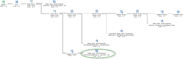
Figure 16-12. The execution plan after creating a new index on Purchasing.PurchaseOrderDetail
Creating the index results in a couple of small changes to the execution plan. Instead of scanning the clustered index on Purchasing.PurchaseOrderDetail, the new index is scanned (circled above). One of the Compute Scalar operations was also eliminated. This is a mild improvement to the plan.
The real question is this: what happened to the performance? The execution time did not radically improve, dropping to 154, an improvement of about 12%. The reads on the Purchasing.PurchaseOrderDetail table dropped from 66 to 31. This is a very modest improvement, and it may not be worth the extra processing time
for the inserts.
Modifying the Procedure
Sometimes, one of the best ways to improve performance is for the business and the developers to work together to reevaluate the needs of a particular query. In this instance, the existing query uses a LIKE clause against the LastName column in the Person.Person table. After checking with the developers, it's determined that this query will be getting its values from a drop-down list that is an accurate list of LastName values from the database. Since the LastName value is coming from the database, the developers can actually get the BusinessEntitylD column from the Person.Person table. This makes it possible to change the procedure so that it now looks like this:
ALTER PROCEDURE dbo.spr_PurchaseOrderBySalesPersonName
@BusinessEntityId int
ASv
SELECT poh.PurchaseOrderID,
poh.OrderDate,
pod.LineTotal,
p.[Name] AS ProductName,
e.JobTitle,
per.LastName + ', ' + per.FirstName AS SalesPerson
FROM Purchasing.PurchaseOrderHeader AS poh
JOIN Purchasing.PurchaseOrderDetail AS pod
ON poh.PurchaseOrderID = pod.PurchaseOrderID
JOIN Production.Product AS p
ON pod.ProductID = p.ProductID
JOIN HumanResources.Employee AS e
ON poh.EmployeeID = e.BusinessEntityID
JOIN Person.Person AS per
ON e.BusinessEntityID = per.BusinessEntityID
WHERE e.BusinessEntityID = @BusinessEntityID
ORDER BY per.LastName,
per.FirstName ;
Use this statement to execute the procedure now:
EXEC dbo.spr_PurchaseOrderBySalesPersonName @BusinessEntityId = 260;
Running this query results in the execution plan shown in Figure 16-13.
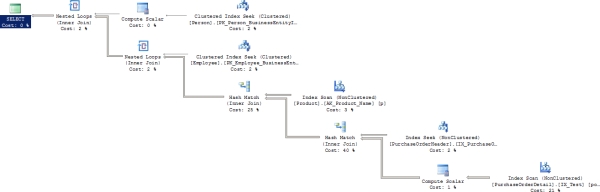
Figure 16-13. The execution plan after rearchitecting the procedure
Many of the operations will be familiar. However, the costs have changed, the order of events has changed, and the plan is actually much simpler now, with close to the bare minimum number of operations. The newReason For Early Termination resulted in Good Enough Plan Found” Best of all, check out the results from the statistics:
SQL Server parse and compile time:
CPU time = 0 ms, elapsed time = 1 ms.
SQL Server Execution Times:
CPU time = 0 ms, elapsed time = 0 ms.
SQL Server parse and compile time:
CPU time = 0 ms, elapsed time = 0 ms.
DBCC execution completed. If DBCC printed error messages, contact your system administrator.
SQL Server Execution Times:
CPU time = 0 ms, elapsed time = 1 ms.
DBCC execution completed. If DBCC printed error messages, contact your system administrator.
SQL Server Execution Times:
CPU time = 0 ms, elapsed time = 3 ms.
SQL Server parse and compile time:
CPU time = 0 ms, elapsed time = 0 ms.
SQL Server parse and compile time:
CPU time = 31 ms, elapsed time = 49 ms.
(631 row(s) affected)
Table 'Worktable'. Scan count 0, logical reads 0, physical reads 0, read-ahead reads 0,
lob logical reads 0, lob physical reads 0, lob read-ahead reads 0.
Table 'PurchaseOrderDetail'. Scan count 1, logical reads 31, physical reads 1,
read-ahead reads 29, lob logical reads 0, lob physical reads 0, lob read-ahead reads 0.
Table 'PurchaseOrderHeader'. Scan count 1, logical reads 3, physical reads 2,
read-ahead reads 0, lob logical reads 0, lob physical reads 0, lob read-ahead reads 0.
Table 'Product'. Scan count 1, logical reads 5, physical reads 1, read-ahead reads 8,
lob logical reads 0, lob physical reads 0, lob read-ahead reads 0.
Table 'Employee'. Scan count 0, logical reads 2, physical reads 2, read-ahead reads 0,
lob logical reads 0, lob physical reads 0, lob read-ahead reads 0.
Table 'Person'. Scan count 0, logical reads 3, physical reads 3, read-ahead reads 0,
lob logical reads 0, lob physical reads 0, lob read-ahead reads 0.
(1 row(s) affected)
SQL Server Execution Times:
CPU time = 15 ms, elapsed time = 166 ms.
SQL Server Execution Times:
CPU time = 46 ms, elapsed time = 215 ms.
SQL Server parse and compile time:
CPU time = 0 ms, elapsed time = 0 ms.
SQL Server Execution Times:
CPU time = 0 ms, elapsed time = 0 ms.
The number of reads has been reduced across the board. The execution time is about the same as the last adjustment, 160ms to 154ms; however, the results illustrate how you can't simply rely on a single execution for measuring performance. Multiple executions showed a more consistent improvement in speed, but nothing radical. The CPU time was about the same at 15 ms. If you change the test and allow the query to use a compiled stored procedure, as is more likely in most production environments, then execution time drops down to 132 ms, and the CPU time drops back down to 15 ms. If you change the test again, to allow for data caching, which may be the case in some environments, execution time drops to 93 ms.
Taking the performance from 435ms to 160ms is not a dramatic improvement because this query is being called only once. If it were called thousands of times a second, getting 2.7 times faster would be worth quite a lot. However, more testing is necessary to reach that conclusion. You need to go back and assess the impact on the overall database workload.
Analyzing the Effect on Database Workload
Once you've optimized the worst-performing query, you must ensure that it doesn't hurt the performance of the other queries; otherwise, your work will have been in vain.
To analyze the resultant performance of the overall workload, you need to use the techniques outlined in Chapter 15. For the purposes of this small test, reexecute the complete workload in --workload and capture extended events in order to record the overall performance.
![]() Tip For proper comparison with the original extended events, please ensure that the graphical execution plan is off.
Tip For proper comparison with the original extended events, please ensure that the graphical execution plan is off.
Figure 16-14 shows the corresponding trace output captured in an extended events file in SSMS.
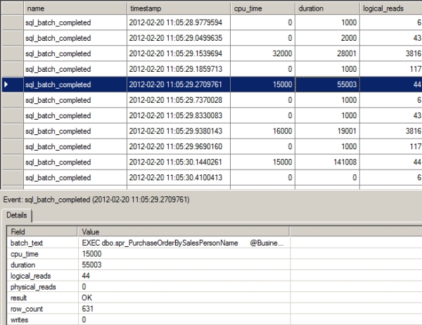
Figure 16-14. The profiler trace output showing the effect of optimizing the costliest query on the complete workload
From this trace, Table 16-6 summarizes the resource use and the response time (i.e., Duration) of the query under consideration.
Table 16-6. Resource Usage and Response Time of the Optimized Query Before and After Optimization
|
Column |
Before Optimization |
After Optimization |
|
Reads |
1901 |
44 |
|
Writes |
0 |
0 |
|
CPU |
31 ms |
15 ms |
|
Duration |
71 ms |
55 ms |
![]() Note The absolute values are less important than the relative difference between the Before Optimization and the corresponding After Optimization values. The relative differences between the values indicate the relative improvement in performance.
Note The absolute values are less important than the relative difference between the Before Optimization and the corresponding After Optimization values. The relative differences between the values indicate the relative improvement in performance.
It's possible that the optimization of the worst performing query may hurt the performance of some other query in the workload. However, as long as the overall performance of the workload is improved, you can retain the optimizations performed on the query.
Iterating Through Optimization Phases
An important point to remember is that you need to iterate through the optimization steps multiple times. In each iteration, you can identify one or more poorly performing queries and optimize the query or queries to improve the performance of the overall workload. You must continue iterating through the optimization steps until you achieve adequate performance or meet your service-level agreement (SLA).
Besides analyzing the workload for resource-intensive queries, you must also analyze the workload for error conditions. For example, if you try to insert duplicate rows into a table with a column protected by the unique constraint, SQL Server will reject the new rows and report an error condition to the application. Although the data was not entered into the table and no useful work was performed, valuable resources were used to determine that the data was invalid and must be rejected.
To identify the error conditions caused by database requests, you will need to include the following in your Extended Events (alternatively, you can create a new session that looks for these events in the errors or warnings category):
- error_reported
- execution_warning
- hash_warning
- missing_column_statistics
- missing_join_predicate
- sort_warning
For example, consider the following SQL queries (--errors in the download):
INSERT INTO Purchasing.PurchaseOrderDetail
(PurchaseOrderID,
DueDate,
OrderQty,
ProductID,
UnitPrice,
ReceivedQty,
RejectedQty,
ModifiedDate
)
VALUES (1066,
'1/1/2009',
1,
42,
98.6,
5,
4,
'1/1/2009'
) ;
GO
SELECT p.[Name],
psc.[Name]
FROM Production.Product AS p,
Production.ProductSubCategory AS psc ;
GO
Figure 16-15 shows the corresponding session output.
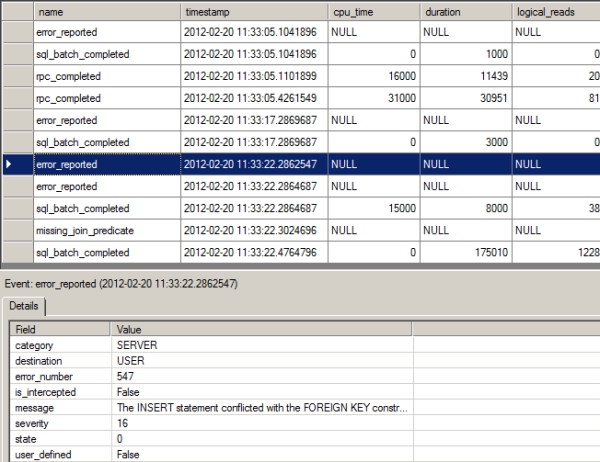
Figure 16-15. Extended Events output showing errors raised by a SQL workload
From the Extended Events output in Figure 16-15, you can see that two errors occurred:
- error_reported
- missing_join_predicate
The error_reported error was caused by the INSERT statement, which tried to insert data that did not pass the referential integrity check; namely, it attempted to insert Productld = 42 when there is no such value in the Production.Product table. From the error_number column, you can see that the error number is 547. The message column shows the full description for the error.
The second type of error, missing_join_predicate, is caused by the SELECT statement:
SELECT p.[Name]
,c.[Name]
FROM Production.Product AS p
,Production.ProductSubCategory AS c;
GO
If you take a closer look at the SELECT statement, you will see that the query does not specify a JOIN clause between the two tables. A missing join predicate between the tables usually leads to an inaccurate result set and a costly query plan. This is what is known as a Cartesian join, which leads to a Cartesian product, where every row from one table is combined with every row from the other table. You must identify the queries causing such events in the Errors and Warnings section and implement the necessary fixes. For instance, in the preceding SELECT statement, you should not join every row from the Production.ProductCategory table to every row in the Production.Product table—you must join only the rows with matching ProductCategorylD, as follows:
SELECT p.[Name]
,c.[Name]
FROM Production.Product AS p
JOIN Production.ProductSubCategory AS c
ON p.ProductSubcategoryID = c.ProductSubcategoryID ;
Even after you thoroughly analyze and optimize a workload, you must remember that workload optimization is not a one-off process. The workload or data distribution on a database can change over time, so you should periodically check whether your queries are optimized for the current situation. It's also possible that you may identify shortcomings in the design of the database itself. Too many joins from overnormalization or too many columns from improper denormalization can both lead to queries that perform badly, with no real optimization opportunities. In this case, you will need to consider redesigning the database to get a more optimized structure.
Summary
As you learned in this chapter, optimizing a database workload requires a range of tools, utilities, and commands to analyze different aspects of the queries involved in the workload. You can use Extended Events to analyze the big picture of the workload and identify the costly queries. Once you've identified the costly queries, you can use the query window and various SQL commands to troubleshoot the problems associated with the costly queries. Based on the problems detected with the costly queries, you can apply one or more sets of optimization techniques to improve the query performance. The optimization of the costly queries should improve the overall performance of the workload; if this does not happen, you should roll back the change or changes.
In the next chapter, I summarize the performance-related best practices in a nutshell. You'll be able to use this information as a quick and easy-to-read reference.