SQL Server supports data compression. Data compression reduces the size of the database, which helps improve query performance because queries on compressed data read fewer pages from the disk and thus use less IO. However, data compression requires extra CPU resources for updates, because data must be decompressed before and compressed after the update. Data compression is therefore suitable for data warehousing scenarios in which data is mostly read and only occasionally updated.

SQL Server supports three compression implementations:

• Row compression: Row compression reduces metadata overhead by storing fixed data type columns in a variable-length format. This includes strings and numeric data. Row compression has only a small impact on CPU resources and is often appropriate for OLTP applications as well.
• Page compression: Page compression includes row compression, but also adds prefix and dictionary compressions. Prefix compression stores repeated prefixes of values from a single column in a special compression information structure that immediately follows the page header, replacing the repeated prefix values with a reference to the corresponding prefix. Dictionary compression stores repeated values anywhere in a page in the compression information area. Dictionary compression is not restricted to a single column.
• Unicode compression: In SQL Server, Unicode characters occupy an average of two bytes. Unicode compression substitutes single-byte storage for Unicode characters that don't truly require two bytes. Depending on collation, Unicode compression can save up to 50 % of the space otherwise required for Unicode strings. Unicode compression is very cheap and is applied automatically when you apply either row or page compression.

You can gain quite a lot from data compression in a data warehouse. Foreign keys are often repeated many times in a fact table. Large dimensions that have Unicode strings in name columns, member properties, and attributes can benefit from Unicode compression.

The following figure explains dictionary compression:

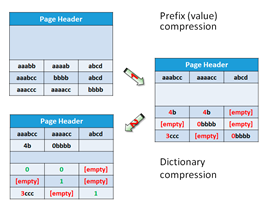
As you can see from the figure, dictionary compression (corresponding to the first arrow) starts with prefix compression. In the compression information space on the page right after the page header, you can find stored prefixes for each column. If you look at the top left cell, the value in the first row, and first column, is aaabb. The next value in this column is aaabcc. A prefix value aaabcc is stored for this column in the first column of the row for the prefix compression information. Instead of the original value in the top left cell, the 4b value is stored. This means use four characters from the prefix for this column and add the letter b to get the original value back. The value in the second row for the first column is empty because the prefix for this column is equal to the whole original value in that position. The value in the last row for the first column after the prefix compression is 3ccc, meaning that in order to get the original value, you need to take the first three characters from the column prefix and add a string ccc, thus getting the value aaaccc, which is, of course, equal to the original value. Check prefix compression for the other two columns also.

After prefix compression, dictionary compression is applied (corresponding to the second arrow in the Dictionary compression figure). It checks all strings across all columns to find common substrings. For example, the value in the first two columns of the first row after the prefix compression was applied is 4b. SQL Server stores this value in the dictionary compression information area as the first value in this area, with index 0. In the cells, it stores just the index value 0 instead of the value 4b. The same happens for the 0bbbb value, which you can find in the second row, second column, and third row, third column, after prefix compression is applied. This value is stored in the dictionary compression information area in the second position with index 1; in the cells, the value 1 is left.

You might wonder why prefix compression is needed. For strings, a prefix is just another substring, so dictionary compression could cover prefixes as well. However, prefix compression can work on nonstring data types as well. For example, instead of storing integers 900, 901, 902, 903, and 904 in the original data, you can store a 900 prefix and leave values 0, 1, 2, 3, and 4 in the original cells.

Now it's time to test SQL Server compression. First of all, let's check the space occupied by the test fact table:

EXEC sys.sp_spaceused N'dbo.FactTest', @updateusage = N'TRUE'; 
GO 

The result is as follows:

Name          rows    reserved  data      index_size  unused
------------  ------  --------  --------  ----------  ------
dbo.FactTest  227981  49672 KB  48528 KB      200 KB  944 KB

The following code enables row compression on the table and checks the space used again:

ALTER TABLE dbo.FactTest  
 REBUILD WITH (DATA_COMPRESSION = ROW); 
EXEC sys.sp_spaceused N'dbo.FactTest', @updateusage = N'TRUE'; 

This time, the result is as follows:

Name          rows    reserved  data      index_size  unused
------------  ------  --------  --------  ----------  ------
dbo.FactTest  227981  25864 KB  24944 KB       80 KB  840 KB

You can see that a lot of space was saved. Let's also check the page compression:

ALTER TABLE dbo.FactTest  
 REBUILD WITH (DATA_COMPRESSION = PAGE); 
EXEC sys.sp_spaceused N'dbo.FactTest', @updateusage = N'TRUE'; 

Now the table occupies even less space, as the following result shows:

Name          rows    reserved  data      index_size  unused
------------  ------  --------  --------  ----------  ------
dbo.FactTest  227981  18888 KB  18048 KB       80 KB  760 KB

If these space savings are impressive to you, wait for columnstore compression! Anyway, before continuing, you can remove the compression from the test fact table with the following code:

ALTER TABLE dbo.FactTest  
 REBUILD WITH (DATA_COMPRESSION = NONE); 

Before continuing with other SQL Server features that support analytics, I want to explain another compression algorithm because this algorithm is also used in columnstore compression. The algorithm is called LZ77 compression. It was published by Abraham Lempel and Jacob Ziv in 1977; the name of the algorithm comes from the first letters of the author's last names plus the publishing year. The algorithm uses sliding window dictionary encoding, meaning it encodes chunks of an input stream with dictionary encoding. The following are the steps of the process:

1. Set the coding position to the beginning of the input stream
2. Find the longest match in the window for the look-ahead buffer
3. If a match is found, output the pointer P and move the coding position (and the window) L bytes forward
4. If a match is not found, output a null pointer and the first byte in the look-ahead buffer and move the coding position (and the window) one byte forward
5. If the look-ahead buffer is not empty, return to step 2

The following figure explains this process via an example:

The input stream chunk that is compressed in the figure is AABCBBABC:

• The algorithm starts encoding from the beginning of the window of the input stream. It stores the first byte (the A value) in the result, together with the pointer (0,0), meaning this is a new value in this chunk.
• The second byte is equal to the first one. The algorithm stores just the pointer (1,1) to the output. This means that in order to recreate this value, you need to move one byte back and read one byte.
• The next two values, B and C, are new and are stored to the output together with the pointer (0,0).
• Then the B value repeats. Therefore, the pointer (2,1) is stored, meaning that in order to find this value, you need to move two bytes back and read one byte.
• Then the B value repeats again. This time, you need to move one byte back and read one byte to get the value, so the value is replaced with the pointer (1,1). You can see that when you move back and read the value, you get another pointer. You can have a chain of pointers.
• Finally, the substring ABC is found in the stream. This substring can be also found in positions 2 to 4. Therefore, in order to recreate the substring, you need to move five bytes back and read 3 bytes, and the pointer (5,3) is stored in the compressed output.