
8
Test Generation Concepts
Whereas Chapters 9 and 10 explore strategies for test data generation, this chapter introduces concepts that help us streamline the discussion of test data generation, by reviewing such questions as the following: How does the target attribute that we are trying to achieve through the test influence test data generation? What requirements does the generated test data satisfy? What criteria can we deploy to generate test data? How do we assess the quality of generated test data (i.e., the extent to which the generated test data fulfills its requirements)? How do we measure test coverage, that is, the extent to which a test achieves its goal?
8.1 TEST GENERATION AND TARGET ATTRIBUTES
In Chapter 7, we have surveyed several different goals of a test operation, and several distinct attributes that a test operation may aim to establish. If we focus exclusively on test processes that aim to establish a functional property (dealing with input/output behavior, rather than performance or resource usage, for example) then we can identify the following possible categories:
- Testing a program to establish correctness with respect to a specification (as in acceptance testing).
- Testing a program to ensure that it computes its intended function (as in unit testing).
- Testing a program to ensure that it is robust (i.e., that it behaves appropriately outside the domain of its specification).
- Testing a program to ensure its safety (i.e., that even when it fails to meet its specification, it causes no safety violations).
- Testing a program to ensure its security, that is, that it meets relevant security requirements, such as confidentiality (ability to protect confidential data from unauthorized disclosure), integrity (ability to protect critical data from unauthorized modification), authentication (ability to authenticate system users), and so on.
In this section, we make the case that all these attributes can be modeled uniformly as the property that the function of the candidate program refines a given specification. What changes from one attribute to another is merely the form of the specification at hand; so that in the sequel, when we talk about testing a candidate program against a specification, we could be talking about any one of these attributes.
We review in turn the five attributes listed earlier and model them as refinement properties with respect to various specifications.
- Correctness: According to Chapter 5, a program p is correct with respect to a specification R if and only if the function P of program p refines relation R.
- Precision: Whereas correctness tests the candidate program against its specification, precision tests the candidate program against the function that it is designed to compute, to which we refer as the intended function of the program. By definition, the intended function of the program is a deterministic relation; for all intents and purposes, being correct with respect to a deterministic specification is indistinguishable from computing the function defined by this specification. Whereas the specification is used for acceptance testing, the intended function of the program is used for unit testing or system testing (depending on scale) where the emphasis is not on proving correct behavior, but rather on finding faults. To illustrate the difference, consider the following simple example: We let space S be defined by positive natural variables x and y, and let specification R on S be defined as follows:
where gcd (x, y) refers to the greatest common divisor of x and y. Assume that upon inspecting the specification, the program designer decides to implement the gcd using Euclid’s algorithm. The intended function is then

If the candidate program fails to deliver gcd (x, y) in variable y during acceptance testing, that does not count as a failure since the specification does not require the condition
 . But if the candidate program fails to deliver gcd(x, y) in variable y during unit testing (when the emphasis is on finding faults), that does count as a failure, since it indicates that the program is not computing its intended function.
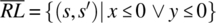
 - Robustness: By definition, a program is said to be robust with respect to a specification if and only if it behaves appropriately (even) in situations for which the specification makes no provisions; we do not have a general definition of what is appropriate behavior, but it should at least encompass normal termination in a well-defined final state, with appropriate alerts or error messages. For a relational specification R, the set of initial states for which the specification makes provisions is RL; hence, the set of states for which it makes no provisions is
 . If we limit ourselves to specification
  for initial states outside the domain of R, it means we merely want candidate programs to terminate normally in such cases; if we want to impose additional appropriateness conditions, we further restrict the behavior of candidate programs outside the domain of R by taking the intersection of
  with some other term, say A. Hence, a program that is correct and robust with respect to R refines the following specification:As an illustration, we consider the space S defined by integer variables x and y, and we consider the following specification:

where gcd (x, y) refers to the greatest common divisor of x and y. If we also want candidate programs to be robust, then we can write a more refined specification under this form:
We find
 ; if we choose to post an error message in x whenever x or y are not positive, we find the following composite specification:
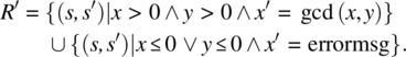
A candidate program is robust if and only if it refines specification R′.
- Safety: By definition, safety means correctness with respect to safety-critical requirements. Most typically, the product specification refines the safety critical requirements; but because safety-critical requirements carry much heavier stakes and their violation costs a great deal more than other requirements, they are the subject of special scrutiny, and are the subject of more thorough testing and verification. From a logical standpoint, safety can be modeled by the property that the function of the program refines the safety-critical requirements.
- Security: By definition, security means correctness with respect to security requirements, such as confidentiality, integrity, authentication, availability, and so on.
Hence, while correctness (with respect to a possibly nondeterministic specification), precision (the property of computing the exact intended function), robustness (the property of behaving appropriately for unexpected situations), safety (the property of avoiding safety violations), and security (the property of evading or mitigating security threats) all sound different, they can all be modeled as the property that the function of the candidate program refines a specification; what varies from one attribute to the next is the specification in question. These specifications are ranked by the refinement ordering as shown in Figure 8.1.
Figure 8.1 A hierarchy of attributes.
Henceforth, we will talk about testing a program against a specification without specifying what form the specification has, hence which attribute we are testing it for.
8.2 TEST OUTCOMES
It is clear, from the foregoing discussions, that when we want to test a program against a specification R, there is no reason to consider test data outside the domain of R. Indeed, even if we are testing the behavior of candidate programs outside their normal operating conditions, as we must do for robustness, this amounts to testing the candidate program for correctness with respect to a more refined specification. We consider the following definition:
The set of initial states on which execution of candidate program p yields a successful outcome is ![]() . This set is clearly a subset of
. This set is clearly a subset of ![]() . We give two examples to illustrate the set of states that yield a successful outcome, for a given specification R and a given program p.
. We give two examples to illustrate the set of states that yield a successful outcome, for a given specification R and a given program p.
We consider a specification R on space S defined by variables x and y of type integer, which is defined as follows:
We let p be the following candidate program on the same space S:
p: {while (y!=0) {y=y-1; x=x+1;}}.
The function P that this program computes on space S is defined as follows:
From this, we find
![]()
= {since ![]() }
}
![]()
= {quantifying over s′, and simplifying}
![]()
Indeed, execution of p on s yields a successful outcome only if ![]() .
.
As a second example, we consider a specification R on space S defined by variables x, y, and z of type integer, which is defined as follows:
We let p be the following candidate program on the same space S:
p: {while (y!=0) {y=y-1; z=z+x;}}.
The function P that this program computes on space S is defined as follows:
From this, we find
![]()
= {by substitution}
![]()
= {simplification}
![]()
= {quantifying over s′, and simplifying}
![]()
Indeed, execution of p on s yields a successful outcome only if ![]() .
.
8.3 TEST GENERATION REQUIREMENTS
The purpose of a test operation is to run a candidate program on sample inputs and observe its behavior in order to draw conclusions about the quality of the program. In general, we cannot make certifiable claims about the quality of the candidate program unless we have observed its execution on all possible inputs under all possible circumstances. Because this is most generally impossible, we must find substitutes; this is the focus of test data generation.
Given a candidate program p and a specification R whose domain is X, we are interested to choose a subset T of X such that we can achieve the goal of the test by executing the candidate program on T rather than on X. Clearly, the requirement that T must satisfy depends on the goal of the test. As we remember from Chapter 7, we identify several possible goals of testing, including the following:
- Finding and removing faults
- Proving the absence of faults
- Estimating the frequency of failures
- Ensuring the infrequency of failures
These goals impose different requirements on T, which we review below:
- A Logical Requirement: Set T must be chosen in such a way that if there exists an input x in X such that a candidate program p fails when executed on x, then there exists t in T such that program p fails when executed on t. This requirement provides, in effect, that set T is sufficiently rich to detect all possible faults in candidate programs.
- A Stochastic Requirement: The reliability observed on the execution of a candidate program p on T is the same as (or an approximation of) the reliability observed on the execution of the candidate program p on X. So that any reliability claim made on the basis of observations made during the testing phase, when input data are limited to T, will be borne out during the operation phase, when the input ranges over all of X.
- A Sufficient Stochastic Requirement: The reliability observed on the execution of a candidate program p on T is lower than, or the same as, the reliability observed on the execution of a candidate program p on X. So that any reliability claim made on the basis of observations made during the testing phase, when input data is limited to T, will be matched or exceeded during the operation phase, when the input ranges over all of X.
Given that the set of states that yield a successful execution of a candidate program p is ![]() , the logical requirement can be expressed as follows:
, the logical requirement can be expressed as follows:
This requirement provides, in effect, that if program p has a fault, test data set T will expose it; as such, this requirement serves the first goal, whose focus is to expose all faults of the program. In order for T to serve the second goal of testing, it needs to satisfy the following condition:
which provides, in effect, that if program p executes successfully on T, then it executes successfully on X (hence is correct). The following proposition provides that these two conditions are equivalent.
This proves that a test set T is adequate for the first goal of testing (finding and removing faults) if and only if it is adequate for the second goal of testing (proving the absence of faults). Figures 8.2, 8.3, and 8.4, respectively, show three configurations of X, ![]() and T: a case where a test data T is certainly inadequate, a case where test data T may be adequate, and a set of two cases where test data T is certainly adequate. The cases where T is provably adequate are both of limited practical interest: one arises when the program is correct, the other arises when T is all of S.
and T: a case where a test data T is certainly inadequate, a case where test data T may be adequate, and a set of two cases where test data T is certainly adequate. The cases where T is provably adequate are both of limited practical interest: one arises when the program is correct, the other arises when T is all of S.
Figure 8.2 Inadequate test data.
Figure 8.3 Possibly adequate test data.
Figure 8.4 Certainly adequate test data.
The test data T of Figure 8.2 is certainly inadequate: The left-hand side of the implications in proposition test data adequacy is valid, but the right-hand side is not.
Test data T of Figure 8.3 may be adequate.
Figure 8.4 shows cases where T is certainly adequate: (a) if p is correct or (b) if T is exhaustive test.
The testing goals can be mapped onto test data requirements as shown in the following table:
| Testing goals | Test data requirements |
| Finding and removing faults | Logical requirement |
| Proving the absence of faults | Logical requirement |
| Estimating the frequency of failures | Stochastic requirement |
| Ensuring the infrequency of failures | Stochastic requirement Sufficient stochastic requirement |
Note that the stochastic requirement logically implies the sufficient stochastic requirement; hence, any test data set that satisfies the former satisfies the latter; for the same reason, the former can be used whenever the latter is adequate. Note that we focus our attention on X, the domain of the specification, rather than the domain (or the state space) of the program, since candidate programs are judged for their behavior on the domain of the specification they are supposed to satisfy.
In practice, it is very difficult to generate test data that meets these requirements, especially the logical requirement; nevertheless, these requirements serve a useful function, in that they define the goal that we must attain as we generate test data, and a yardstick by which we judge the quality of our choices. In the next section, we discuss the concept of a test selection criterion, which is a criterion by which we characterize test data to satisfy some requirement among the three introduced in this section.
8.4 TEST GENERATION CRITERIA
Given a test generation requirement, among the three we have discussed earlier, it is common to generate a test generation criterion, that is, a condition on set T that dictates how to generate it in such a way as to satisfy the requirement.
For the logical requirement, the most compelling (and most common) criterion is to partition the domain of the specification by an equivalence relation, say EQ, and to mandate that T contain one representative element for each equivalence class of X modulo EQ. Formally, these conditions are written as follows:
The first condition provides that each equivalence class of X modulo EQ is represented by at least one element of T, as illustrated in Figure 8.5 (where the equivalence classes are represented by the quadrants). As for the second condition, it merely provides that T contains no unnecessary elements, that is, no two elements of the same equivalence class.
Figure 8.5 Partitioning the domain of the specification.
The rationale for this criterion depends on the definition of EQ: Ideally, EQ is defined in such a way that all the elements of the same equivalence class of X modulo EQ have the same fault diagnosis capability, that is, either the candidate program runs successfully on all of them or it fails on all of them; hence, there is no reason to test candidate programs on more than one element per equivalence class. Formally, this condition can be written as follows:
We refer to this condition (on EQ) as the condition of partition testing, and we have the following proposition.
The condition ![]() provides, in effect, that each element of X is related to at least one element of T; in other words, each equivalence class of X modulo EQ has a representative in T. As for the condition
provides, in effect, that each element of X is related to at least one element of T; in other words, each equivalence class of X modulo EQ has a representative in T. As for the condition ![]() , it is not needed for the proof of this proposition, because it only limits the size of T (it provides that no more than one representative per equivalence class is needed in T). In practice, the hypothesis that EQ does indeed satisfy this property is usually hard to support, and the criterion is only as good as the hypothesis.
, it is not needed for the proof of this proposition, because it only limits the size of T (it provides that no more than one representative per equivalence class is needed in T). In practice, the hypothesis that EQ does indeed satisfy this property is usually hard to support, and the criterion is only as good as the hypothesis.
For the stochastic requirement and the sufficient stochastic requirement, the most common generation criterion that we invoke provides that set T has the same probability distribution as the expected usage pattern of the software product. The rationale for this criterion is to imitate the operating conditions of the software product to the largest extent possible, so that whatever behavior we observe during testing is sure to be borne out during the product’s operation. Given a specification R whose domain is X, we consider the following criterion on a subset T of X: We let χ be a random variable on X that reflects the usage pattern of candidate programs in operation, and we let θ be a random variable on T that reflects the distribution of test data during the testing phase. Then the probability distribution pθ of θ over T must be identical to the probability distribution pχ of χ over X, in the following sense:
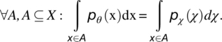
The probability of occurrence of a test data point in any sub set A of X is identical to the probability of occurrence of an actual input data point in subset A during typical system operation. As an additional requirement, T must also be large enough so that observations of the candidate program on T provide a statistically significant sample of the program’s behavior. In practice, depending on how large (or how dense) T is, it may be impossible to define a probability distribution pθ that mimics exactly the probability distribution pχ; we then let distribution pθ approximate the probability distribution pχ (Fig. 8.6).
Figure 8.6 Mimicking a probability distribution.
In order to mimic the probability distribution pχ, set T must have more elements where pχ is high than where pχ is low. This matter will be revisited in Chapter 9, when we discuss random test generation.
8.5 EMPIRICAL ADEQUACY ASSESSMENT
Whereas in the foregoing discussions, we have attempted to characterize the adequacy of a test data T with respect to test selection requirements by means of analytical arguments, in this section we consider empirical arguments. Specifically, we ponder the question: How can we assess the ability of a test set T to expose faults in candidate programs? A simple-minded way to do this is to run candidate programs on a test set T and see what proportion of faults we are able to expose; the trouble with this approach is that we do not usually know what faults a program has. Hence, if execution of program p on test set T yields no failures, or few failures, we have no way to tell whether this is because the program has no (or few) faults or because test set T is inadequate. To obviate this difficulty, we generate mutants of program p, which are programs obtained by making small changes to p, and we run all these mutants on test set T; we can then assess the adequacy of test set T by its ability to distinguish all the mutants from the original p, and to distinguish them from each other. A note of caution is in order, though: it is quite possible for mutants to be indistinguishable, in the sense that the original program p and its mutant compute the same function; in such cases, the inability of set T to distinguish the two programs does not reflect negatively on T. This means that in theory, we should run this experiment only on mutants which we know to be distinct (i.e., to compute a different function) from the original; but because it is very difficult in practice to tell whether a mutant does or does not compute the same function as the original, we may sometimes (for complex programs) run the experiment on the assumption that all mutants are distinct from the original, and from each other.
As an illustrative example, we consider the following sorting program, which we had studied in Chapter 6; we call it p.
void somesort (itemtype a[MaxSize], indextype N) // line 1{ // 2indextype i; i=0; // 3while (i<=N-2) // 4{indextype j; indextype mindx; itemtype minval; // 5j=i; mindx=j; minval=a[j]; // 6while (j<=N-1) // 7{if (a[j]<minval) {mindx=j; minval=a[j];} // 8j++;} // 9itemtype temp; // 10temp=a[i]; a[i]=a[mindx]; a[mindx]=temp; // 11i++;} // 12} // 13
Imagine that we have derived the following test data to test this program:
| T | Index N | Array a[..] | Comment/rationale |
| t1 | 1 | [5] | Trivial size |
| t2 | 2 | [5,5] | Borderline size, identical elements |
| t3 | 2 | [5,9] | Borderline size, sorted |
| t4 | 2 | [9,5] | Borderline size, inverted |
| t5 | 6 | [5,5,5,5,5,5] | Random size, identical elements |
| t6 | 6 | [5,7,9,11,13,15] | Random size, sorted |
| t7 | 6 | [15,13,11,9,7,5] | Random size, inverted |
| t8 | 6 | [9,11,5,15,13,7] | Random size, random order |
The question we ask is: How adequate is this test data? If we run our sorting routine on this data and all executions are successful, how confident can we be that our program is correct? The approach advocated by mutation testing is to generate mutants of program p by making small alterations to its source code and checking to what extent the test data is sensitive to these alterations. Let us, for the sake of argument, consider the following mutants of program p:
void m1 (itemtype a[MaxSize], indextype N) // line 1{ // 2indextype i; i=0; // 3while (i<=N-1) // changed N-2 into N-1 // 4{indextype j; indextype mindx; itemtype minval; // 5j=i; mindx=j; minval=a[j]; // 6while (j<=N-1) // 7{if (a[j]<minval) {mindx=j; minval=a[j];} // 8j++;} // 9itemtype temp; // 10temp=a[i]; a[i]=a[mindx]; a[mindx]=temp; // 11i++;} // 12} // 13
void m2 (itemtype a[MaxSize], indextype N) // line 1{ // 2indextype i; i=0; // 3while (i<=N-2) // 4{indextype j; indextype mindx; itemtype minval; // 5j=i; mindx=j; minval=a[j]; // 6while (j<=N-1) //changed <=into < // 7{if (a[j]<minval) {mindx=j; minval=a[j];} // 8j++;} // 9itemtype temp; // 10temp=a[i]; a[i]=a[mindx]; a[mindx]=temp; // 11i++;} // 12} // 13
void m3 (itemtype a[MaxSize], indextype N) // line 1{ // 2indextype i; i=0; // 3while (i<=N-2) // 4{indextype j; indextype mindx; itemtype minval; // 5j=i; mindx=j; minval=a[j]; // 6while (j<=N-1) // 7{if (a[j]< =minval) {mindx=j; minval=a[j];}//changed < into <= // 8j++;} // 9itemtype temp; // 10temp=a[i]; a[i]=a[mindx]; a[mindx]=temp; // 11i++;} // 12} // 13
void m4 (itemtype a[MaxSize], indextype N) // line 1{ // 2indextype i; i=1; // changed 0 into 1 // 3while (i<=N-2) // 4{indextype j; indextype mindx; itemtype minval; // 5j=i; mindx=j; minval=a[j]; // 6while (j<=N-1) // 7{if (a[j]<minval) {mindx=j; minval=a[j];} // 8j++;} // 9itemtype temp; // 10temp=a[i]; a[i]=a[mindx]; a[mindx]=temp; // 11i++;} // 12} // 13
void m5 (itemtype a[MaxSize], indextype N) // line 1{ // 2indextype i; i=0; // 3while (i<=N-2) // 4{indextype j; indextype mindx; itemtype minval; // 5j=i; mindx=j; minval=a[j]; // 6while (j<=N-1) // 7{if (a[j]<minval) {mindx=j; minval=a[j];} // 8j++;} // 9itemtype temp; // 10a[i]=a[mindx]; temp;=a[i]; a[mindx]=temp;// inverted the first two statements // 11i++;} // 12} // 13
Given these mutants, we now run the following test driver, which considers the mutants in turn and checks whether test set T distinguishes them from the original program p.
void main (){for (int i=0; i<=5; i++) // does T distinguish// mutant (i) from p{for (int j=1; j<=8; j++) // is p(tj) different from mi(tj)?{load tj onto N, a;run p, store result in a’;load tj onto N, a;run mutant i, compare outcome to a’;}if one of the tj returned a different outcome from p, announce:“mutant i distinguished”else announce: “mutant i not distinguished”;}}; // assess T according to how many mutants were distinguished
The actual source code for this is shown in the appendix. Execution of this program yields the following output, in which we show for each test datum tj and for each mutant mi whether execution of the mutant on the datum yields a different result from execution of the original program p on the same datum.
| Mutants | ||||||
| T | m1 | m2 | m3 | m4 | m5 | |
| t1 | True | True | True | True | True | |
| t2 | True | True | True | True | True | |
| t3 | True | True | True | True | True | |
| t4 | True | True | True | False | False | |
| t5 | True | True | True | True | True | |
| t6 | True | True | True | True | True | |
| t7 | True | True | True | False | False | |
| t8 | True | True | True | False | False | |
| Mutant distinguished? | No | No | No | Yes | Yes | |
Before we make a judgment on the adequacy of our test data set, we must first check whether the mutants that have not been distinguished from the original program are identical to it or not (i.e., compute the same function). For example, it is clear from inspection of the source code that mutant m1 is identical to program p: indeed, since program p sorts the array by selection sort, then once it has selected the smallest ![]() elements of the array, the remaining element is necessarily the largest; hence, the array is already sorted. What mutant m1 does is to select the Nth element of the array and permute it with itself—a futile operation, which program p skips. Mutant m3 also appears to compute the same function as the original program p, though it selects a different value for variable
elements of the array, the remaining element is necessarily the largest; hence, the array is already sorted. What mutant m1 does is to select the Nth element of the array and permute it with itself—a futile operation, which program p skips. Mutant m3 also appears to compute the same function as the original program p, though it selects a different value for variable mindx when the array contains duplicates; this difference has no impact on the overall function of the program. The question of whether mutant m2 computes the same function as the original program is left as an exercise.
In general, once we have ruled out mutants that are deemed to be equivalent to the original program, we must consider the mutants that the test data did not distinguish from the original program even though they are distinct and raise the question: What additional test data should we generate to distinguish all these mutants? Conversely, we can view the proportion of distinct mutants that the test data has not distinguished as a measure of inadequacy of the test data, a measure that we should minimize by adding extra test data or refining existing data.
Note that the test data t1, t2,t3,t5, and t6 does not appear to help much in testing the sorting program, as they are unable to distinguish any mutant from the original program.
In addition to its use to assess test sets, mutation is also used to automatically correct minor faults in programs, when their specification is available and readily testable: one can generate many mutants and test them against the specification using an adequate test set, until it encounters a mutant that satisfies the specification. There is no assurance that such a mutant can be found, nor that only one mutant can be found to satisfy the specification, nor that a mutant that satisfies the specification is more correct than the original program; nevertheless, this technique may find some uses in practice.
8.6 CHAPTER SUMMARY
From this chapter, it is important to remember the following ideas and concepts:
- One does not generate test data in an ad hoc manner; rather, one generates test data to fulfill specific requirements, which depend on the goal of the test. We have identified several possible requirements that a test data set must satisfy.
- It is customary to articulate a test data generation criterion, as a first step in test data generation; this criterion defines what condition a test data must satisfy to meet a selected requirement.
- Any test data selection criterion must be assessed with respect to the target requirement: To what extent does the criterion ensure that the requirement is fulfilled? This is usually very difficult to ascertain, but having well-defined requirements, even if they are not ever fulfilled, serves as a yardstick against which we can assess criteria.
- The adequacy of a criterion can be assessed analytically, by referring to the targeted requirement, or empirically, using mutants. A test data set is all the more adequate for finding program faults that it is capable of distinguishing the candidate program against mutants thereof (obtained by slight modifications).
- The only mutants that should be used to assess the adequacy of a test data set are those that are functionally distinct from the original candidate program. But determining whether a mutant is or is not functionally equivalent to the original program can take a great deal of effort, and may be error prone.
8.7 EXERCISES
- 8.1. Consider the following specification Ron space S defined by integer variables x, y and z:
and consider the following program p (whose function is P) on the same space:
{while (y!=0) {y=y-1; z=z+x;}}.Compute
 , and interpret your results.
 - 8.2. Same question as Exercise 8.1, for the space and specification, and the following program:
{z=0; while (y!=0) {y=y-1; z=z+x;}}. - 8.3. Same question as Exercise 8.1, for the space and specification, and the following program:
{z=0; while (y>0) {y=y-1; z=z+x;}}. - 8.4. Consider the following specification R on space S defined by integer variables x, y and z:

and consider the following program p(whose function is P) on the same space:
{while (y!=0) {y=y-1; z=z+x;}}.Compute
 , and interpret your results.
 - 8.5. Same question as Exercise 8.4, for the space and specification, and the following program:
{z=0; while (y!=0) {y=y-1; z=z+x;}}. - 8.6. Same question as Exercise 8.4, for the space and specification, and the following program:
{z=0; while (y>0) {y=y-1; z=z+x;}}. - 8.7. Consider the following specification R on space S defined by integer variables x, y and z:

and consider the following program p (whose function is P) on the same space:
{while (y!=0) {y=y-1; z=z+x;}}.Compute
 , and interpret your results.
 - 8.8 Same question as Exercise 8.7, for the space and specification, and the following program:
{z=0; while (y!=0) {y=y-1; z=z+x;}}. - 8.9 Same question as Exercise 8.7, for the space and specification, and the following program:
{z=0; while (y>0) {y=y-1; z=z+x;}}. - 8.10. Consider the mutant m2 in the example discussed in Section 8.5. If this mutant is identical to the original program p, explain why. If not, find additional test data to distinguish it from p.
- 8.11. Consider the following sorting program; generate five mutants for it and perform the same analysis as we present in Section 8.5, using the same test data. If you conclude that the test data is inadequate for the mutants you generate, generate additional test data.
void insertSort(int a[], int length){int i, j, value;for(i = 1; i < length; i++){value = a[i];for (j = i - 1; j >= 0 && a[j] > value; j--){a[j + 1] = a[j];}a[j + 1] = value;}}
8.8 BIBLIOGRAPHIC NOTES
The concept of test data selection criterion is due to Goodenough and Gerhart (1975). The concept of program mutations and mutation testing is due to Richard Lipton; an early presentation of the topic is given in DeMillo et al. (1978).
8.9 APPENDIX: MUTATION PROGRAM
void m1 (int a[6], int N);void m2 (int a[6], int N);void m3 (int a[6], int N);void m4 (int a[6], int N);void m5 (int a[6], int N);void m6 (int a[6], int N);void loaddata (int j);// state variablesint a[6];int N;int aa[9][7];int Na[9];int ap[6];int main (){Na[1]=1; aa[1][1]=5;Na[2]=2; aa[2][1]=5; aa[2][2]=5;Na[3]=2; aa[3][1]=5; aa[3][2]=9;Na[4]=4; aa[4][1]=9; aa[4][2]=5;Na[5]=6; aa[5][1]=5; aa[5][2]=5; aa[5][3]=5; aa[5][4]=5;aa[5][5]=5; aa[5][6]=5;Na[6]=6; aa[6][1]=5; aa[6][2]=7; aa[6][3]=9; aa[6][4]=11;aa[6][5]=13; aa[6][6]=15;Na[7]=6; aa[7][1]=15; aa[7][2]=13; aa[7][3]=11; aa[7][4]=9;aa[7][5]=7; aa[7][6]=5;Na[8]=6; aa[8][1]=9; aa[8][2]=11; aa[8][3]=5; aa[8][4]=15;aa[8][5]=13; aa[8][6]=7;for (int i=1; i<=5; i++) // does T distinguish mutant (i) from p{bool discumul; discumul=true;for (int j=1; j<=8; j++) // is p(tj) different from mi(tj)?{// load tj onto N, a;bool dis; dis=true;loaddata(j);p(a,N);for (int k=0; k<N; k++) {ap[k]=a[k];}// load tj onto N, a;loaddata(j);switch(i) {case 1: m1(a,N); xcase 2: m2(a,N);case 3: m3(a,N);case 4: m4(a,N); case 5: m5(a,N);}for (int k=0; k<N; k++) {dis = dis && (a[k]==ap[k]);}if (dis) {cout << “ test t” << j << “ returns True”<< endl;}else {cout << “ test t” << j << “ returns False”<< endl;}discumul=discumul && dis;}if (discumul) {cout << “mutant ” << i << “ not distinguishedfrom p.” << endl;}else {cout << “mutant ” << i << “ distinguished from p.”<< endl;}};}void loaddata(int j){N=Na[j];for (int k=0; k<N; k++) {a[k]=aa[j][k+1];}}