13
Test Outcome Analysis
After we have gone through the trouble of generating test data, deriving a test oracle, designing a test driver, running/deploying the test, and collecting data about the test outcome, it is appropriate to ask the question: what claim can we now make about the program under test? This is the question we focus on in this chapter. The answer to this question depends, in fact, on the goal of the testing activity, which in turn affects the testing process as well as the conclusions that can be drawn therefrom.
We argue that if we test a software product without consideration of why are we doing it and what claims we can make about the product at the end of the test, then we are wasting our time. Testing a software product for the sole purpose of removing faults at random, in the absence of an overarching V&V plan, may be counterproductive for several reasons: First, because of the risks that we may be introducing faults as fast as we are removing other faults, or faster; second, because we have more faith in a software product in which we have not encountered the first fault than in a software product in which we have removed ten faults (hence our faith in the product may have dropped rather than risen as a result of the test); third, because faults have widely varying impacts on failure, hence are not equally worthy of our attention (we ought to budget our testing effort and maximize our return on investment by removing high impact faults before low impact faults).
We distinguish between two broad types of claims (of unequal value) that one can make from a testing activity:
- Logical claims
- Stochastic claims
We review these in turn, below.
13.1 LOGICAL CLAIMS
13.1.1 Concrete Testing
We consider the scenario where we run a candidate program g on space S against an oracle derived from specification R, and we find that the program runs successfully on all elements of the test data set T; then we ask the question: what claims can be made about program g?
Before we answer this question, we need to specify precisely what we mean by runs successfully (in reference to a program under test). The first interpretation we adopt is that whenever the test oracle is executed, it returns true; we have no assurance that the oracle will ever be invoked (in particular, if the program under test does not terminate), but we know that if it is ever invoked, it returns true. Under this interpretation of a successful test, we observe that in order for the oracle to be invoked, the program g has to terminate its execution, that is, the initial state has to be an element of dom(G). Hence we write:
We rewrite this expression, replacing oracle(t, G(t)) by its expression as a function of the specification R (refer to the derivation of oracles from specifications, discussed in Chapter 9):
By logical simplification, we transform this as follows:
By changing the quantification, we rewrite this as follows:
By logical simplification, we rewrite this as follows:
By tautology, we rewrite this as follows:
If we let R′ be the pre-restriction of R to T, we can write this as:
In other words, we have proven that program g is partially correct with respect to R′, the pre-restriction of R to T. Whence the following proposition:
Because the domain of R′ is typically a very small subset of the domain of R, this property is in effect very weak, in general. Yet, logically, this is all we can claim from the successful execution of the test; it is possible that the successful test gives us some confidence in the quality/reliability of the software product, but that is not a logical property.
13.1.2 Symbolic Testing
Symbolic testing is, in general very complex, for not only does it involve complex control structures such as loops, loops with complex loop bodies, nested loops, and so on, but it may also involve complex data structures. In order to model complex data structures, we need a rich vocabulary of relevant abstractions, as well as an adequate axiomatization pertaining to these abstractions.
Not only is symbolic testing complex and error prone, it is often wasteful and inefficient: Indeed, it is very common for programs to be much more refined than the specification they are intended to satisfy; hence by trying to compute the function of a program in all its minute detail, we may be dealing with functional detail that is ultimately irrelevant to the specification that the program is written to satisfy and even more irrelevant to the specification that the program is being tested against. Consider the example of a binary search, which searches an item x in an ordered array a by means of two indices l and h (for low and high), and imagine having to characterize the final values of l and h as a function of a and x; it is very difficult, as it depends on very minute details of the program (whether strict or loose inequalities are used) on whether x is in a or not, and on the position of x with respect to cells of a; and yet it is also of little relevance as the most important outcome of the search is to determine whether x is in a, and eventually at what location. Performing the symbolic execution of a binary search just to check whether it satisfies the specification of a search is like going through an 8000 feet pass to climb a 3000 feet peak.
If we do overcome the complexity, the error proneness, and the possibility of excessive (and irrelevant) detail that come with full blown symbolic execution of a program, then our reward is that we can prove any property we wish about the program in question, with respect to any specification we wish to consider. As a reminder, we present below a brief summary of the properties that we may want to prove about a candidate program g on space S once we have computed its function G.
13.1.3 Concolic Testing
From a cursory analysis, it appears that
- Concrete testing, to the extent that it is carried out without fault removal, typically produces a very weak logical statement, pertaining to partial correctness with respect to a typically weak specification.
- Symbolic Execution, to the extent that it is deployed in full, enables us to prove any property we wish with respect to any specification, but it is very difficult to deploy, is very prone to errors, and forces us to deal with functional detail that may well be irrelevant to whatever property we wish to prove.
These two methods can be compared and contrasted in the following table.
| Method | Process | Assumption | Scope | Assessment | ||
| Advantages | Drawbacks | |||||
| Concrete testing | Dynamic execution and analysis | Faithful reflection of actual operating conditions | No limitation | Ease of deployment | Weak claims | |
| Symbolic execution | Static analysis of the source code, impact of execution on symbolic data | Rules used for symbolic execution consistent with actual behavior of computer | Limited to aspects of programs that are easy to model | Arbitrarily strong claims with respect to arbitrary specifications | Difficulty/complexity/error proneness of deployment | |
Concolic testing is a technique that combines concrete testing and symbolic testing in an effort to achieve a greater return on investment than each method taken individually; the name concolic is in fact derived from combining the beginning of concrete with the ending of symbolic.
Concolic testing is essentially a form of concrete testing, where the program is executed on actual test data, but it uses symbolic execution techniques to compute the path conditions of various execution paths through the program, hence improves the coverage of the test. By focusing on execution paths rather than closed form control structures, and by targeting the derivation of path conditions rather than fully detailed path functions, concolic testing obviates the main difficulties of symbolic testing. On the other hand, by taking a systematic approach to the derivation of path conditions, it aims to achieve a degree of efficiency by ensuring that each new concrete test data exercises a new execution path, rather than a previously visited execution path.
13.2 STOCHASTIC CLAIMS: FAULT DENSITY
It appears from the previous section that testing does not yield much in terms of logical claims: Concrete testing yields very weak logical claims (in terms of partial correctness with respect to very partial specifications), while symbolic testing may yield stronger claims of correctness with respect to arbitrary specifications, provided we have extracted the function of candidate programs in all its minute detail (a tedious, complex, error-prone, and potentially wasteful task). In this and the following sections, we consider stochastic claims, which focus on likely properties rather than logically provable properties.
The first stochastic property we consider is fault density. A technique known as fault seeding consists in injecting faults into the source code of the candidate program and then submitting the program to a test data set T and counting:
- The number of seeded faults that have been uncovered and
- The number of unseeded faults that have been uncovered.
If we assume that the test data we have used detects the same proportion of seeded faults as unseeded faults, we can use this information to estimate the number of unseeded faults in the program. Specifically, if we let:
- D be the number of faults seeded into the program,
- D′ be the number of seeded faults that were discovered through test data T,
- N′ be the number of native faults that were discovered through test data T, and
- N be the total number of native faults in the program,
Then we can estimate the total number of native faults, say N, by means of the following formula:
Whence we can infer
This formula assumes that test T is as effective at finding seeded faults as it is at finding native faults (see Fig. 13.1) and the estimation is only as good as the assumption. Hence for example, if we seed 100 faults (![]() ) and we find that our test detects 70 faults of which 20 are seeded faults (
) and we find that our test detects 70 faults of which 20 are seeded faults (![]() ), we estimate the number of native faults as follows:
), we estimate the number of native faults as follows:
Figure 13.1 Fault distribution (native vs. seeded).
This approach is based on the assumption that test T is as effective at exposing seeded faults as it is at exposing native faults. If we do not know enough about the type of native faults that the program has, or about the effectiveness of the test data set T to expose seeded and native faults, then we can use an alternative technique.
The alternative technique, which we call cross testing, consists in generating two test data sets of equivalent size, where the goal of each test is to expose as many faults as possible, then to analyze how many faults they expose in fact, and how many of these two sets of faults are common. We denote by:
- T1 and T2 the two test data sets.
- F1 and F2 the set of faults exposed by T1 and T2 (respectively); by abuse of notation, we may use F1 and F2 to designate the cardinality of the sets, in addition to the sets themselves.
- Q the number of faults that are exposed by T1 and by T2.
- N the total number of faults that we estimate to be in the software product.
If we consider the set of faults exposed by T2, we can assume (in the absence of other sources of knowledge) that test data set T1 catches the same proportion of faults in T2 as it catches in the remainder of the input space (Fig. 13.2). Hence we write:
Figure 13.2 Estimating native faults.
From which we infer:
If test data T1 exposes 70 faults and test data T2 exposes 55 faults from which 30 are already exposed by T1 then we estimate the number of faults in the program to be:
So far we have discussed fault density as though faults are independent attributes of the software product, which lend themselves to precise enumeration; in reality, faults are very dependent on each other so that removing one fault may well affect the existence, number, location, and nature of the other faults; this issue is addressed in the exercises at the end of the chapter. It is best to view fault density as an approximate measure of product quality rather than a precise census of precisely identified faults. Not only is the number of faults itself vaguely defined (see the discussions in Chapter 6), but their impact on failure rate varies widely in practice (from 1 to 50 according to some studies); hence a program with 50 low impact faults may be more reliable than a program with one high impact fault; this leads us to focus on failure probability as the next stochastic claim we study.
13.3 STOCHASTIC CLAIMS: FAILURE PROBABILITY
13.3.1 Faults Are Not Created Equal
In Section 13.1, we have discussed logic claims that can be made on the basis of testing a software product, and in Section 13.2 we have discussed probabilistic claims on the likely number of faults in a software product. In this section, we consider another probabilistic claim, namely failure probability (the probability of failure of any single execution) or the related concept of failure frequency (expected number of failures per unit of operation time); there are a number of conceptual and practical arguments to the effect that failure frequency is a more significant attribute of a software product than fault density.
- Not only is fault an evasive, hard to define, concept, as we have discussed in Chapter 6, but so is the concept of fault density. The reason is that faults are not independent attributes of the product but are rather highly interdependent. Saying that there are 30 black marbles in a bucket full of (otherwise) white marbles means that once we remove these 30 black marbles, we are left with a bucket of uniformly white marbles. But saying that we have 30 faults in a software product ought to be understood as an approximate indicator of product quality; whenever one of these faults is removed, this may affect the existence, number, location and/or nature of the other faults. Removing one black marble from a bucket that has 30 black marbles in the midst of white marbles leaves us with 29 black marbles, but removing a fault from a program that has 30 faults does not necessarily leave us with 29 faults (due to the interactions between faults).
- From the standpoint of a product’s end-user, failure frequency is a much more meaningful measure of product quality/reliability than fault density. A typical end-user is not cognizant of the structure and properties of the software product, and hence cannot make any sense of an attribute such as fault density. But failure frequency is meaningful, for it pertains to an observable/actionable attribute of the software product: a passenger who boards an aircraft for a 3-hour flight may well know that aircrafts sometimes drop from the sky accidentally, but she/he does board anyway, because she/he estimates that the mean time to failure of the aircraft is so large that the likelihood that a failure happens over the duration of the flight is negligible.
- Faults have widely varying impacts on product reliability. Some faults cause the software product to fail at virtually every execution, whereas others may cause it to fail under a very specific set of circumstances that arises very seldom (e.g., specific special cases of exception handling). Consequently, faults are not equally worthy of the tester’s attention; in order to maximize the impact of the testing effort, testers ought to target high impact faults before lower impact faults. One can achieve that by pursuing a policy of reducing failure rates rather than a policy of reducing fault density. A key ingredient of this policy is to test the software product under the same circumstances as its expected usage profile; this ensures that the reliability growth that we observe through the testing phase will be borne out during the operational phase of the product.
Figure 13.3 shows the difference between testing a product according to its expected usage profile and testing it with a different profile; the horizontal axis represents time and the vertical axis represents the observed failure rate of the software product; the vertical line that runs across the charts represents the end of the testing phase and the migration of the software product from its test environment to its field usage environment. If we test the product according to its usage profile (by mimicking whatever circumstances it is expected to encounter in the field) then the observation of reliability growth during test (as a result of fault removal) will be borne out once the product has migrated to field usage, because most of the faults that the user is likely to expose (sensitize) have already been exposed and removed; this is illustrated in the upper chart. If the product has been tested under different circumstances from its usage profile, then the tester likely removed many faults that have little or no impact on the user, while failing to remove faults that end users are likely to expose/sensitize; hence when the product is delivered, its failure rate may jump due to residual high impact faults.
Figure 13.3 Impact of usage patterns.
- If a fault is very hard to expose, it may well be because it is not worth exposing. Consider, as a simple example, a software product that is structured as an alternative between two processing components: one (say, A) for normal circumstances and one (say, B) for highly exceptional circumstances. Imagine that in routine field usage, component B is called once for every ten thousand (10000) times more often than A is called. Then we ought to focus our attention on removing faults from A until the most frequent fault of B becomes more likely to cause failure than any remaining fault in A (Fig. 13.4).
Figure 13.4 Targeted test coverage.
So that if faults in B prove to be very difficult to expose because executing B requires a set of very precise circumstances that are difficult to achieve, the proper response may be to focus on testing A until B becomes the bottleneck of reliability, rather than to invest resources in removing faults in B at the cost of neglecting faults in A that are more likely to cause failure.
For all these reasons, estimating the number of faults in a software product is generally of limited value; in the remainder of this section, we focus our attention on estimating failure frequency rather than fault density.
13.3.2 Defining/Quantifying Reliability
The reliability of a software product reflects, broadly speaking, the product’s likelihood of operating free of failure for long periods of time. Whereas correctness is a logical property (a program is or is not correct), reliability is a probabilistic property (quantifying the likelihood that the program operates failure free for some unit of time). The first matter that we need to address in trying to define reliability is to decide what concept of time we are talking about. To this effect we consider three broad classes of software products, which refer to three different scales of time:
- A process control system, such as a system controlling a nuclear reactor, a chemical plant, an electric grid, a telephone switch, a flight control system, an autonomous vehicle, and so on. Such systems iterate constantly through a control loop, whereby they probe sensors, analyze their input along with possible state data, compute control parameters and feed them to actuators. For such systems, time can be measured by clock time or possibly by the number of iterations that the system goes through; these two measures are related by a linear formula, since the sampling time for such system is usually fixed (e.g., take a sample of sensor data every 0.1 second).
- A transaction processing system, such as an e-commerce system, an airline reservation system, or an online query system. Such system operates on a stimulus–response cycle, whereby they await user transactions, and whenever a transaction arises, they process it, respond to it, and get ready for the next transaction. Because such systems are driven by user demands, there is no direct relation between actual time and the number of transaction cycles they go through; for such systems, the passage of time can be measured by the number of transactions they process.
- Simple input/output programs, which carry no internal state, and merely compute an output from an input provided by a user, whenever they are invoked. For such software product, time is equated with number of invocations/executions.
Hence when we talk about time in the remainder of this chapter, we may be referring to different measures for different types of programs.
Another matter that we must pin down prior to discussing reliability is the matter of input to a program; referring back to the distinction made earlier about three families of software products, we observe that only the third family of software products operates exclusively on simple inputs; software products in the other two families operate on state information in addition to the current input data. When we talk about the input to a program, we refer generally to input data provided by the user as well as relevant state data or context/environment data.
As a measure of failure avoidance over time, reliability can be quantified in a number of ways, which we explore briefly:
- Probability that the execution of the product on a random input completes without failure.
- Mean time to the next failure.
- Mean time between failures.
- Mean number of failures for a given period of time.
- Probability of failure free-operation for a given period of time.
It is important to note that reliability is always defined with respect to an implicit (or sometimes, explicit) user profile (or usage pattern). A user profile is defined by a probability distribution over the input space; if the input space is a discrete set, then the probability distribution is defined by means of a function from the set to the interval [0.0 .. 1.0]; if the set is a continuous domain, then the probability distribution is defined by a function whose integral over the input space gives 1.0 (the integral over any subset of the input space represents the probability that the input falls in that subset). User profile (or usage pattern) is important in the study of reliability because the same system may have different reliabilities for different user profiles.
It is common, in the study of reliability, to classify failures into several categories, depending on the impact of the failure, ranging from minor inconvenience to a catastrophic impact involving loss of life, mission failure, national security threats, and so on. We postpone this aspect of the discussion to Section 13.4, where we explore an economic measure of reliability, which refines the concept of failure classification.
13.3.3 Modeling Software Reliability
A software reliability model is a statistical model that represents the reliability of a software product as a function of relevant parameters; each model can be characterized by the assumptions it makes about relevant parameters, their properties, and their impact on the likelihood of product failure. It is customary to classify reliability models according to the following criteria:
- Time Domain. Some models are based on wall clock time whereas others measure time in terms of the number of executions.
- Type. The type of a model is defined by the probability distribution function of the number of failures experienced by the software product as a function of time.
- Category. Models are divided into two categories depending on the number of failures they can experience over an infinite amount of operation time: models for which this number is finite and models for which it is infinite.
- For Finite Failures Category. Functional form of the failure intensity in terms of time.
- For Infinite Failures Category. Functional form of the failure intensity in terms of the number of observed failures.
We consider the reliability of a system under the assumption that the number of failures it can experience is finite, and we let M(t) be the random variable that represents the number of failures experienced by a software product from its first execution (or from the start of its test phase) to time t. We denote by μ(t) the expected value of M(t) at time t and we assume that μ(t) is a non-decreasing, continuous, and differentiable function of t and we let λ(t) be the derivative of μ(t) with respect to time:
This function represents the rate of increase of function μ(t) with time; we refer to it the failure intensity (or the failure rate) of the software product. If this failure rate is constant (independent of time), which is a reasonable assumption so long as the software product is not modified (no fault removal) and its operating conditions (usage pattern) are maintained, then we find:
for some constant c; given that time ![]() corresponds to the first execution of the product under observation, no failures are observed at
corresponds to the first execution of the product under observation, no failures are observed at ![]() , hence we find
, hence we find ![]() .
.
A common model of software reliability for constant failure intensity provides the following equation between failure, intensity, time, and the probability of failure free operation:
The probability F(t) that the system has failed at least once by time t is the complement of R(t), that is,
The probability density function f(t) of probability F(t) is the derivative of F(t) with respect to time, which is:
The probability that a failure occurs between time t0 and time t1 is given by the following integral:
The probability that a failure occurs before time t is a special case of this formula, for ![]() and
and ![]() , which yields:
, which yields:
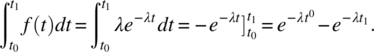
which is what we had found earlier using the definition of R(t). The mean time to failure of the system can be estimated by integrating, for t from 0 to infinity, the function that represents the product of t by the probability that the failure occurs at time t. We write this as:
We compute this integral using integration by parts:
= {integration by parts}
= {evaluating the second term, which is zero at both ends}
= {simple integral}
= {value at zero}
We highlight this result:
This equation enables us to correlate the mean time to failure with all the relevant probabilities of system failure. For example, the following table shows the probability that the system operates failure-free for a length of time t, for various values of t, assuming that the system’s mean time to failure is 10,000 hours:
| Operation time, t (in hours) | Probability of failure free operation |
| 0 | 1.0 |
| 1 | 0.9999 |
| 10 | 0.999 |
| 100 | 0.99005 |
| 1,000 | 0.904837 |
| 10,000 | 0.367879 |
| 100,000 | 4.53999 × |
| Probabilities of failure free operation for MTTF = 10,000 hours | |
From this table, we can estimate the probability that a failure occurs in each of the intervals indicated in the table below, by virtue of the formula
where ![]() designates the probability that the failure occurs between time t0 and time t1.
designates the probability that the failure occurs between time t0 and time t1.
| Operation time, t (in hours) | Probability of failure free operation |
| Within the first hour | 0.0001 |
| After the first hour, within 10 hours | 0.0009 |
| After the first 10 hours, within 100 hours | 0.00895 |
| After the first 100 hours, within 1,000 hours | 0.085213 |
| After the first 1,000 hours, within 10,000 hours | 0.536958 |
| After the first 10,000 hours, within 10,0000 hours | 0.367834 |
| After the first 100, 000 hours | 0.0000454 |
| Total | 1.0 |
| Probabilities of failure per interval of operation time, for MTTF = 10, 000 hours | |
13.3.4 Certification Testing
Imagine that we must test a software product to certify that its reliability meets or exceeds a given value; this situation may arise at acceptance testing if a reliability standard is part of the product requirements. If the candidate program passes a long enough test without any failure, we ought to certify it; the question that arises, of course, is how long does the program have to run failure-free to be certified. The length of the certification test depends on the following parameters:
- The target reliability standard, which we quantify by the MTTF (or its inverse, the failure intensity).
- The discrimination ratio (γ), which is the tolerance of error we are willing to accept around the estimate of the target reliability; for example, if the target reliability is 10,000 hours and we are willing to certify a product whose actual reliability is 8,000, or to reject a product whose actual reliability is 12,500, then γ = 1.25.
- The producer risk (α), which is the probability that the producer tolerates of having his product rejected as unreliable even though it does meet the reliability criterion.
- The consumer risk (β), which is the probability that the consumer tolerates of accepting a product that has been certified even though it does not meet the reliability criterion.
The length of the certification test is given by the following formula:
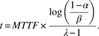
As an illustrative example, assume that the target reliability MTTF has been fixed at 10,000 hours and the discrimination ratio γ has been fixed at 1.25. Further, assume that:
- The producer tolerates no more than a probability of 0.1 that his product be unfairly/inadvertently declined (due to estimation errors) even though its reliability actually exceeds 12,500 hours; this means α is given value 0.1.
- Due to the criticality of the application, the consumer tolerates no more than a probability of 0.06 that his product be inadvertently accepted (due to estimation errors) even though its actual reliability falls below 8,000; this means β is given value 0.06.
Using this data, we find that the size of the certification test set:
If we were to run this test in real-time, this would take about 12 years; but of course we do not have to, provided we have an estimate of the number of times that the product is invoked per hour, say N, then we convert hours into number of executions/invocations, and we obtain the number of tests we must run the program on, say n:
a much more realistic target.
13.3.5 Reliability Estimation and Reliability Improvement
The purpose of this section is to discuss how we can use testing to estimate the reliability of a software product and how to use testing and fault removal to improve the reliability of a product up to a predefined standard.
If we are given
- a software product,
- a specification that describes its requirements,
- an oracle that is derived from the specification, and
- a usage profile of the product in the form of a probability distribution over the domain of the specification,
then the simplest way to estimate its reliability is to run the product on randomly generated test data according to the given usage profile, to record all the failures of the product, and to compute the average time (number of tests/executions) that elapses between successive failures. One may argue that what we are measuring herein is actually the MTBF rather than the MTTF; while we agree that strictly speaking this experiment is measuring the MTBF, we argue that it provides an adequate indication of the mean time to failure.
The simple procedure outlined herein applies when the software product is unchanged throughout the testing process and our purpose is to estimate its mean time to failure as is. We now consider the case of a software product which is due to undergo a system-level test for the purpose of removing faults therein until the system’s reliability reaches or exceeds a target reliability requirement. This process applies to the aggregate made up of the following artifacts:
- the software product under test,
- the specification against which the product is being tested, and the oracle that is derived from this specification,
- a usage profile of the product in the form of a probability distribution over the domain of the specification,
- a target reliability requirement that the product must reach or exceed upon delivery, in the form of a MTTF,
and iterates through the following cycle until the estimated product reliability reaches or exceeds the target MTTF requirement:
- Run the software product on randomly generated test data according to the product’s anticipated usage pattern and deploy the oracle derived from the selected specification, until a failure is disclosed by the oracle.
- Analyze (off-line) the failure, identify the fault that caused it, and remove it.
- Compute a new estimate of the product reliability, in light of the latest removed fault.
The first step of this iterative process can be automated by means of the following test driver:
void testRun (int runLength){stateType initS, s; bool moreTests;runLength=0; moreTests=true;while moreTests{generateRandom(s); inits=s; runLength++;g(); // modifies s, preserves initSmoreTests = oracle(initS,s);}runLength--;}
The second step is carried out off-line; each execution of the test driver and removal of the corresponding fault is referred to as a test run. As for the third step, a question of how we estimate/update the reliability of the software product after each test run is raised. The obvious (and useless) answer to this question is: it depends on what fault we have removed; indeed, we know that the impact of faults on reliability varies a great deal from one fault to another; some faults cause more frequent failures than others, hence their removal produces a greater increase in reliability.
Cleanroom reliability testing assumes that each fault removal increases the mean time to failure by a constant amount starting from a base value and uses the testing phase to estimate the initial mean time to failure as well as the ratio by which the mean time to failure increases after each fault removal. This model is based on the following assumptions:
- Unit testing is replaced by static analysis of the source code, using verification techniques similar to those we discuss in Chapter 5.
- Reliability testing replaces integration testing and applies to the whole system, in which no part has been previously tested.
- Reliability testing records all executions of the system starting from its first execution.
It we let MTTF0 be the mean time to failure of the system upon its integration and we denote by MTTFN the mean time to failure of the system after the removal of the N first faults (resulting from the N first failures), then we can write (according to our modeling assumption):
where R is the reliability growth factor, which reflects by what multiplicative factor the MTTF grows, on average, after each fault is removed. At the end of N runs, we know what N is, of course; we need to determine the remaining constants, namely MTTF0 and R. To determine these two constants, we use the historic data we have collected on the N first runs, and we take a linear regression on the logarithmic version of the equation above:
We perform a linear regression where log(MTTFN) is the dependent variable and N is the independent variable. For the sake of argument, we show in the following table a sample record of a reliability test, where the first column shows the ordinal of the runs and the second column shows the length of each run (measured in terms of the number of executions before failure).
| N | Inter-failure run | Log |
| 0 | 24 | 1.33 |
| 1 | 20 | 1.30 |
| 2 | 36 | 1.56 |
| 3 | 400 | 2.60 |
| 4 | 510 | 2.71 |
| 5 | 10000 | 4.0 |
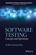
In the third column, we record the logarithm of the length of the test runs. When we perform a regression using the third column as dependent variable and the first column as independent variable, we find the following result:
Figure 13.5 gives a graphic representation of the regression, on a logarithmic scale. The least squares linear regression gives the Y intercept and the slope of the regression as follows:
Figure 13.5 Regression log(MTTF) by N.
From this, we infer the mean time to failure at the conclusion of the testing phase as follows:
In other words, if this software product is delivered in its current form, it is expected to execute 3725 times before its next failure. If this reliability attains or exceeds the required standard, then the testing phase ends; else, we proceed with the next test run.
13.3.6 Reliability Standards
So far in this chapter, we have discussed how to certify a product to a given reliability standard or how to improve a product to meet a particular reliability standard, but we have not discussed how to set such reliability standards according to the application domain or to the stakes that are involved in the operation of the software product; this matter is the focus of this section. Broadly speaking, industry standards provide for $1 per hour for tolerable financial losses; the following table shows the required reliability of a software product as a function of the financial loss that a system failure causes.
| Stakes/cost of failure ($) | Required reliability, MTTF |
| $1 | 1 hour |
| $10 | 10 hours |
| $100 | 4 days |
| $1,000 | 6 weeks |
| $1,000,000 | 114 years |
When human lives are at stake, the default industry standard is that the MTTF must exceed typical life expectancy; if more than one life is at stake, this value must be adjusted accordingly. The following table, due to Musa (1999 ), shows the link between mean time to failure values and the probability of failure free operation for 1 hour:
| Mean time to failure | Probability of failure free operation for 1 hour |
| 1 hour | 0.368 |
| 1 day | 0.959 |
| 100 hours | 0.990 |
| 1 week | 0.994 |
| 1 month | 0.9986 |
| A month and a half | 0.999 |
| A year | 0.99989 |
13.3.7 Reliability as an Economic Function
So far we have made several simplifying assumptions as we analyze the reliability of a software product; in this section, we tentatively challenge these assumptions and offer a more refined definition of reliability that lifts these restrictive assumptions:
- We have assumed that the stakeholders in the operation of a software product are a monolithic community, with a common stake in the reliable behavior of the system. In reality, a system may have several different stakeholders, having widely varying stakes in its reliable operation. Hence reliability is best viewed, not as a property of the product, but rather as an attribute of a product and a stakeholder. We represent it, not by a scalar (the MTTF), but rather as a vector, which has one entry per relevant stakeholder.
- We have assumed that the specification is a monolith, which carries a unique stake for each stakeholder, when in fact typical specifications are aggregates of several sub-specifications, representing distinct requirements whose stakes for any given stakeholder may vary widely. Hence whereas in the previous section we talked about the cost of a system failure as an attribute of the system, in this section we consider the structure of a specification, and we associate different costs to different sub-specification, for each stakeholder.
- We have assumed that failure is a Boolean condition, whereby an execution either fails or succeeds, when in fact failure is rather a composite event, where the same system may succeed with respect to some requirements but fail with respect to others. Hence in estimating probabilities of failure, we do not consider failure as a single event, but rather as different events, having possibly different probabilities of occurrence and carrying different stakes even for the same stakeholder (let alone for different stakeholders).
To take into account all these dimensions of heterogeneity, we consider the random variable FC(H), which represents, for stakeholder H, the cost per unit of time that she/he stands to incur as a result of possible system failures (FC stands for failure cost), and we let MFC(H) be the mean of variable FC(H) over various instances of system operation. To fix our ideas, we quantify MFC(H) in terms of dollars per hour of operation, which we abbreviate by $/h. With this measure, it is no longer necessary to distinguish between reliability (freedom from failure with respect to common requirements) and safety (freedom from failure with respect to high stakes requirements), since the mean failure cost takes into account the costs associated with all relevant requirements, ranging from low stakes requirements to high stakes requirements.
We consider a system whose community of stakeholders includes n members H1, H2, H3, … Hn, and whose specification R is structured as the aggregate of several requirements, say
and we let ![]() be the probabilities that the system fails to satisfy requirements R1, R2, R3, … Rm during a unitary operation time (say, 1 hour of operation time). If we let ST(Hi, Rj) be the stakes that stakeholder Hi has in meeting requirement Rj, then the mean failure cost of stakeholder Hi can be approximated by the following formula:
be the probabilities that the system fails to satisfy requirements R1, R2, R3, … Rm during a unitary operation time (say, 1 hour of operation time). If we let ST(Hi, Rj) be the stakes that stakeholder Hi has in meeting requirement Rj, then the mean failure cost of stakeholder Hi can be approximated by the following formula:
This formula is not an exact estimate of the mean failure cost but is an approximation thereof; this stems from two reasons, both of which result from the fact that specifications R1, R2, R3, … Rm are not orthogonal, but rather overlap:
- Costs are not additive: when we consider the costs associated with failure to satisfy two distinct requirements Ri and Rj, the same loss may be counted twice because the two specifications are not totally orthogonal, hence their failures represent related events.
- Probabilities are not multiplicative: If we consider two distinct specification components Ri and Rj that are part of the system specification, failure with respect to Ri and failure with respect to Rj are not statistically independent because the same error may cause both events.
Hence strictly speaking, the formula above is best understood as an upper bound of the mean failure cost, rather than an exact estimate; nevertheless, we use it as a convenient (easy to compute) approximation. We recast the formula of MFC given above in matrix form, by means of the following notations:
- We let MFC be the column vector that has one entry per stakeholder, such that MFC(Hi) represents the mean failure cost of stakeholder Hi.
- We let P be the column vector that has one more entry than there are specification components, such that P(Rj) represents the probability that the system fails to satisfy requirement Rj during a unitary execution time (e.g., 1 hour) and the extra entry represents the probability that no requirement is violated during a unitary execution time.
- We let ST be the matrix that has as many rows as there are stakeholders and as many columns as there are specification components and such that ST(Hi, Rj) represents the loss that stakeholder Hi incurs if requirement Rj is violated; we consider an additional column that represents the event that no requirement is violated.
Then the formula of mean failure cost can be written in relational form as follows (where • represents matrix product):
As a simple (and simple-minded) illustrative example, we consider the flight control system of a commercial aircraft, and we list in turn, a sample of its stakeholders, a sample of its requirements, then we try to fill the stakes matrix (ST) and the failure probability vector (P). For a sample of stakeholders, we cite the following:
- PL: The aircraft pilot
- PS: A passenger
- LIF: The passenger’s life insurance company
- AC: The airline company that operates the aircraft
- AM: The aircraft manufacturer
- INS: The insurance company insuring the aircraft
- FAA: The Civil Aviation Authority (e.g., FAA),
- NGO: An environmental NGO
- RES: A resident in the neighborhood of the origin or destination airport
Among the (massively overlapping and very partial/anecdotal) requirements, we consider the following:
- AP: Adherence to the autopilot settings within acceptable tolerance thresholds
- SM: Smoothness of the transition between different autopilot settings
- ECO: Maximizing fuel economy
- NOI: Minimizing noise pollution
- CO2: Minimizing CO2 pollution
- SAF: Safety critical requirements
We review the stakeholders in turn and discuss for each, the stakes they have in each requirement, as well as a tentative quantification of these stakes in dollar terms; specifically, the quantitative figure represents the amount of money that a stakeholder stands to lose if the cited requirement is violated. In the column labeled XS, we write X if the quantification is deemed exact and S if it is deemed a mere estimate.
The Pilot:
| Requirement | Stake | XS | Value ($) |
| AP | Professional obligation | S | 100.00 |
| SM | Professional satisfaction, personal comfort | S | 60.00 |
| ECO | Professional satisfaction, loyalty to employer | S | 40.00 |
| NOI | Professional satisfaction, good citizenship | S | 30.00 |
| CO2 | Environmental consciousness, good citizenship | S | 70.00 |
| SAF | Professional duty, own safety | S | 1.0 M |
The Passenger:
| Requirement | Stake | XS | Value ($) |
| AP | No direct stake, so long as safety is not at stake | S | 0.00 |
| SM | Personal comfort | S | 60.00 |
| ECO | No direct stake | X | 0.00 |
| NOI | No direct stake | X | 0.00 |
| CO2 | Reducing carbon footprint | S | 40.00 |
| SAF | Personal safety | S | 1.0 M |
The Passenger’s Life Insurance Company:
| Requirement | Stake | XS | Value ($) |
| AP | Indirect impact, through increased risk | S | 80.00 |
| SM | No direct stake | X | 0.00 |
| ECO | No direct stake | X | 0.00 |
| NOI | No direct stake | X | 0.00 |
| CO2 | No direct stake | X | 0.00 |
| SAF | Life Insurance Payout | X | 1.0 M |
The Airline Company that operates the aircraft:
| Requirement | Stake | XS | Value ($) |
| AP | Indicator of Fleet Quality | S | 1000.00 |
| SM | Positive Passenger Experience | S | 800.00 |
| ECO | Direct Pocketbook impact | X | 700.00 |
| NOI | Good corporate citizenship, PR value | S | 400.00 |
| CO2 | Good corporate citizenship, promotional value | S | 600.00 |
| SAF | Loss of aircraft, civil liability, corporate reputation, etc | X | 15.0 M |
The Aircraft Manufacturer:
| Requirement | Stake | XS | Value ($) |
| AP | Pilot confidence in aircraft quality | S | 1000.00 |
| SM | Positive Passenger Experience, impact on corporate reputation | S | 800.00 |
| ECO | Lower Operating Costs as a Sales Pitch | S | 800.00 |
| NOI | Good corporate citizenship, adherence to civil regulations | S | 900.00 |
| CO2 | Good corporate citizenship, corporate image | S | 800.00 |
| SAF | Corporate reputation, viability of aircraft, civil liability | X | 120.0 M |
The Insurance Company Insuring the Aircraft:
| Requirement | Stake | XS | Value ($) |
| AP | Indirect impact on safety | S | 1000.00 |
| SM | No direct stake | X | 0.00 |
| ECO | No direct stake | X | 0.00 |
| NOI | No direct stake | X | 0.00 |
| CO2 | No direct stake | X | 0.00 |
| SAF | Insurance Payout (price of aircraft + $1 M/passenger) | X | 350.0 M |
The Civil Aviation Authority:
| Requirement | Stake | XS | Value ($) |
| AP | Core agency mission | S | 1000.00 |
| SM | No direct stake | X | 0.00 |
| ECO | No direct stake | X | 0.00 |
| NOI | Secondary agency mission | S | 200.00 |
| CO2 | Secondary agency mission | S | 200.00 |
| SAF | Core agency mission | X | 1000.00 |
An Environmental NGO:
| Requirement | Stake | XS | Value ($) |
| AP | No direct stake | X | 0.00 |
| SM | No direct stake | X | 0.00 |
| ECO | No direct stake | X | 0.00 |
| NOI | Secondary organizational mission | S | 100.00 |
| CO2 | Core organizational mission | S | 600.00 |
| SAF | No direct stake | X | 0.00 |
A Resident in the Proximity of the Relevant Airports:
| Requirement | Stake | XS | Value ($) |
| AP | Indirect stake, due to safety implications | S | 200.00 |
| SM | No direct stake | X | 0.00 |
| ECO | No direct stake | X | 0.00 |
| NOI | Viability of home, home value | S | 2000.00 |
| CO2 | Secondary homeowner/health concern | S | 20.00 |
| SAF | Indirect stake, due to safety implications | S | 200.00 |
In light of this discussion, we find the following Stakes matrix, where the column labeled NOF refers to the event that no failure has occurred during a unitary operation time.
| AP | SM | ECO | NOI | CO2 | SAF | NOF | |
| PL | 100 | 60 | 40 | 30 | 70 | 1,000,000 | 0 |
| PS | 0 | 60 | 0 | 0 | 40 | 1,000,000 | 0 |
| LIF | 80 | 0 | 0 | 0 | 0 | 1,000,000 | 0 |
| AC | 1000 | 800 | 700 | 400 | 600 | 15,000,000 | 0 |
| AM | 1000 | 800 | 800 | 900 | 800 | 120,000,000 | 0 |
| INS | 1000 | 0 | 0 | 0 | 0 | 350,000,000 | 0 |
| FAA | 1000 | 0 | 0 | 200 | 200 | 1,000 | 0 |
| NGO | 0 | 0 | 0 | 100 | 600 | 0 | 0 |
| RES | 200 | 0 | 0 | 200 | 20 | 200 | 0 |
As for computing the vector of probabilities, we advocate to proceed as follows:
- Design oracles for each of the requirements introduced above.
- Run reliability tests of the software product to estimate the reliability of the product with respect to each relevant requirement.
- Use the estimates of reliability to determine the probability that the product fails during a unitary operation time (e.g., 1 hour of operation).
For the sake of illustration, we consider the following vector of probabilities:
| Requirement | Probability of failure per hour |
| AP | 0.01 |
| SM | 0.01 |
| ECO | 0.005 |
| NOI | 0.005 |
| CO2 | 0.008 |
| SAF | 0.0000001 |
| NOF | 0.9619999 |
Computing the product of the stakes matrix with the probability vector, we find the following vector of mean failure costs, which has one entry per stakeholder and is quantified in dollars per hour.
| Stakeholder | Mean failure cost ($/hour) |
| PL | 2.61 |
| PS | 1.02 |
| LIF | 0.90 |
| AC | 29.80 |
| AM | 44.90 |
| INS | 45.00 |
| FAA | 12.60 |
| NGO | 5.30 |
| RES | 3.16 |
This table represents, for each stakeholder, the mean of their loss, per hour of operation, as a result of possible system failure; this quantity is measured in dollars per hour and can be used to make economically justified decisions.
13.4 CHAPTER SUMMARY
Testing is useless unless it can help us reach relevant, verifiable conclusions about the product under test. The purpose of this chapter is to survey the various uses of a software test, in terms of the claims that can be made about the product. We consider in turn a number of claims:
- Logical Claims: The successful execution of a program under test on a given test data set can be used as the basis of a claim of correctness of the product with respect to the specification that gives rise to the test oracle. The trouble with such claims is that they pertain to specifications that are very weak, hence are of little value.
- Probabilistic Claims: Fault Density. Testing can be used in conjunction with some assumptions on fault patterns in the program to estimate the density of faults in candidate products. The trouble with this approach is that fault density, even when estimated with great precision, is only tenuously correlated with failure frequency; and from the standpoint of a user, failure frequency is the only meaningful measure of product quality.
- Probabilistic Claims: Failure Frequency. Carefully designed testing experiments can be used to estimate the failure frequency of a product and can also be used to enhance (lower) failure frequency beyond (below) a target value. Once we know the failure frequency of a software product, we can compute a number of relevant reliability attributes, such as the probability of failure within a given time interval, or the mean time to failure.
Once we know the failure frequency of a software product with respect to a given product requirement, and the stakes that a stakeholder has in meeting that requirement, we can estimate the mean of the random variable that represents the loss that the stakeholder stands to incur as a result of possible system failure with respect to that requirement. If we integrate with respect to all the requirements, we obtain the system’s mean failure cost for each stakeholder, measured in dollars per unit of time.
13.5 EXERCISES
- 13.1 Consider the discussion of Section 13.1.1 and revisit its conclusion under the assumption that a successful execution of the test means that for all test cases (elements of T), the candidate program does terminate and the oracle, when invoked, returns true.
- 13.2 If you seed 65 faults into your software product and test it using test data T, which exposes 70 faults of which 30 are seeded, how many faults do you estimate to exist in your product prior to removing all the exposed faults? How many do you estimate to exist after removal of all exposed faults?
- 13.3 If you run your program on two test data sets, say T1 and T2, and you find that T1 exposes 65 faults, and T2 exposes 58 faults of which 28 are also exposed by T1, how many faults do you estimate to exist in your product prior to removing all the exposed faults? How many do you estimate to exist after removal of all exposed faults?
- 13.4 A flight control system has a mean time to failure with respect to safety critical requirements of 20,000 hours.
- If you take a 5 hour flight from Newark to Los Angeles, what is the likelihood that the system will experience a safety critical failure during your flight?
- If the aircraft operates 8 hours a day of actual flying time, what is the likelihood that it will experience a safety critical violation on a given day?
- If the aircraft operates 8 hours a day of actual flight and is grounded for maintenance one day a month, what is the likelihood that it will experience a safety critical failure in its first ten years of operation?
- Under the conditions cited above, what is the likelihood that its first safety critical failure occurs during its 11th year of operation?
- 13.5 We want to certify the reliability of a software product to the MTTF standard of 25,000 executions.
- Given a discrimination ratio of 1.5, a producer risk of 0.25 and a consumer risk of 0.15, how long does the certification test have to be?
- This software product is used to control an industrial process in which data is sampled every minute, analyzed, and actuators are adjusted accordingly. What is the probability that this product will operate failure-free during its first year of operation?
- 13.6 Consider a software product undergoing a process of reliability testing, whereby it is repeatedly tested on randomly generated test data until it fails, the failure is analyzed to identify and remove the presumed fault causing the failure. Assume that the successive test runs that this experiment gives rise to are as follows:
Number of faults removed Number of executions between failures 0 14 1 48 2 36 3 260 4 1,020 5 8,060 6 10,435 Estimate the failure intensity of this product with respect to the selected oracle, in terms of number of executions. If this product is invoked every ten minutes around the clock, what is the mean time to failure of this product in days and in months (assuming 30 days per month)?
- 13.7 Consider a software product that has a mean time to failure of 10 months.
- What is the probability that this product will fail within its first hour of operation?
- What is the probability that this product will fail within its first day of operation?
- What is the probability that this product will fail within its first month of operation?
- What is the probability that this product will fail within its first year of operation?
- What is the probability that this product will fail within its 6th month of operation?
- 13.8 Consider a cloud computing infrastructure of a cloud services provider.
- Identify classes of typical stakeholders.
- Identify typical system requirements.
- Estimate the corresponding stakes matrix.
- Consider a realistic probability distribution of system failures, assuming the system may not fail with respect to more than one requirement per unit of time (e.g., an hour).
- Estimate the mean failure cost of the system with respect to all the stakeholders.
13.6 PROBLEMS
- 13.1 Consider that the fault seeding technique of fault density estimation assumes that faults are independent of each other and that one can identify a number of faults and then remove them. But the remedy to each fault may very well depend on previously removed faults. Explore the consequences of this premise on the technique of fault seeding.
- 13.2 Consider that the cross testing technique of fault density estimation assumes that faults are independent of each other and that one can identify a number of faults and then remove them. But the remedy to each fault may very well depend on previously removed faults. Explore the consequences of this premise on the technique of cross testing.
13.7 BIBLIOGRAPHIC NOTES
For more information on software reliability engineering, consult Musa (1999) and O’Connor (2002). A recent snapshot of the state of the art in symbolic testing is given by Cadar and Sen (2013); note that in this reference, as well as in many references on symbolic execution, the focus is on individual execution paths rather than a comprehensive view of the program; as a result, loops are usually unfurled and converted into an arbitrary number of iterations and treated as sequence (rather than captured by means of Mills’ Theorem, as we do in this chapter). Concolic testing was introduced by Larson and Austin (2003); for an example of a concolic testing paradigm, refer Sen et al. (2005). The technique of Fault Seeding introduced in Section 13.1.1 is due to Harlan D. Mills (1972); as for the technique of fault density estimation by cross-testing, it is due to Shari Laurence Pfleeger and Joanne M. Atlee (2009).