
10
Structural Criteria
Whereas the functional criteria discussed in Chapter 9 generate test data by analyzing the specification of the product, the techniques we discuss in this chapter do so by analyzing the source code of the product. Structural test generation criteria may sound counter-intuitive, since they are using the program to test the program. It is like recruiting the prime suspect in a crime to help in the crime investigation; in the same way that the criminal will bias the investigation away from himself, a faulty program may focus the attention of the tester away from its shortcomings. This is not an idle comparison: Consider that if the program fails to make provisions for half of the input data that it is supposed to process (a massive gap), no amount of structural testing will expose this fault; only by referring back to the specification can we uncover such a failure. More generally, when we endeavor to verify a program, our main resource is redundancy (redundancy between a program and its specification, redundancy between two presumably equivalent programs, redundancy between a program and an executable specification, redundancy between a program and a test oracle, etc.); if we use a program to test the same program, we have no redundancy to depend on. On the other hand, consider that in order to make any claim about the functional attributes of candidate programs, a test-generation strategy must focus on the domain of the specification as a starting point; to the extent that structural test generation analyzes the program rather than its specification, such information is not available.
With these qualifications in mind, we focus our attention in this chapter on generating test data by analyzing the candidate programs; the broad rationale for this type of approach is that if we want to test a program for the purpose of exposing its possible faults, it is sensible to try to exercise all its features, such as all its statements, all its conditions, all its paths, etc. We may argue, in fact, that while functional criteria are more effective at proving the absence of faults (or at least the infrequency of failures caused by these faults), structural criteria are more effective at finding faults, since they focus on the source of the faults.
10.1 PATHS AND PATH CONDITIONS
10.1.1 Execution Paths
Now that we are interested in structural test data generation, we need to look at programs rather than specifications. We assume that our programs are written in a traditional C-like programming language, which includes the following statements:
- Variable declarations, of the form
<data type><variable name>. - Labeled statements, of the form
<label>: <statement>. - Assignment statements, of the form
<variable name> = <expression>. - Sequence statements, of the form
<statement1> ; <statement2>. - Conditional statements, of the form
if <condition><statement>. - Alternation statements, of the form
if <condition><statement1> else <statement2>. - Iteration statements, of the form
while <condition><statement>. - Statement blocks, of the form
{<statement>}. - Function calls, of the form
<function name> ( <parameter list> ).
Because we use structured constructs exclusively, any program is executed in sequence from the first statement to the last statement (we have no exits or return statements in the middle of a program). Hence all executions of our programs start from the first statement and proceed through the code according to the outcome of the various conditions that appear therein. Hence the following definitions.
As an application, we consider the following program and write some of its paths. Note that the definition of paths does not stipulate that they start from the beginning of the programs nor that they end with its last statement, as we want to have the liberty to define partial paths through the code. Nevertheless the sample paths we show below start at the first statement of the program and end at its last statement.
Program g:
{int x; int y; read(x); read(y); // assuming x>0, y>0while (x!=y) {if (x>y) {x=x-y;} else {y=y-x;}};write(x);}
Sample paths through this program include the following:
-
p0: int x; int y; read(x); read(y);
((x!=y)? false); write(x); -
p1: int x; int y; read(x); read(y);
    ((x!=y)? true); ((x>y)? true); x=x-y;
((x!=y)? false); write(x); -
p2: int x; int y; read(x); read(y);
    ((x!=y)? true); ((x>y)? false); y=y-x;
((x!=y)? false); write(x); -
p3: int x; int y; read(x); read(y);
    ((x!=y)? true); ((x>y)? true); x=x-y;
    ((x!=y)? true); ((x>y)? true); x=x-y;
((x!=y)? false); write(x); -
p4: int x; int y; read(x); read(y);
    ((x!=y)? true); ((x>y)? false); y=y-x;
    ((x!=y)? true); ((x>y)? false); y=y-x;
((x!=y)? false); write(x); -
p5: int x; int y; read(x); read(y);
    ((x!=y)? true); ((x>y)? true); x=x-y;
    ((x!=y)? true); ((x>y)? false); y=y-x;
((x!=y)? false); write(x); -
p6: int x; int y; read(x); read(y);
    ((x!=y)? true); ((x>y)? false); y=y-x;
    ((x!=y)? true); ((x>y)? true); x=x-y;
((x!=y)? false); write(x); -
p7: int x; int y; read(x); read(y);
    ((x!=y)? true); ((x>y)? true); x=x-y;
    ((x!=y)? true); ((x>y)? false); y=y-x;
    ((x!=y)? true); ((x>y)? true); x=x-y;
((x!=y)? false); write(x); -
p8: int x; int y; read(x); read(y);
    ((x!=y)? true); ((x>y)? false); y=y-x;
    ((x!=y)? true); ((x>y)? true); x=x-y;
    ((x!=y)? true); ((x>y)? false); y=y-x;
    ((x!=y)? false); write(x);
and so on. Each path represents a trace of execution through the original program.
10.1.2 Path Functions
The following definition introduces the semantics of paths, in terms of the function that they define on their space.
- The effect of each variable declaration of the form “
<type> x” is to change the state of the program from what it was prior to the declaration (say, S) to S ×<type>. - We assume that prior to any variable declarations, the space of the program is limited to two implicit state variables, namely the input stream and the output stream; both of these can be modeled as sequences, where
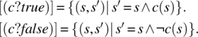
read(x)returns the first element of the input stream and removes it therefrom, whilewrite(x)appends x to the output stream. - The semantics of an assignment statement is defined by:where def(E) is the set of states on which E can be evaluated, and the symbol _ stands for all the other (than x) variables of the space.

- The semantics of a condition is defined by the following equations:
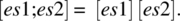
- The semantics of sequence is defined by the following equation:
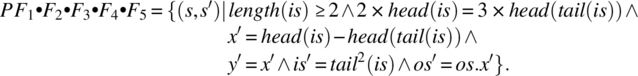
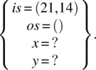
As an illustration of these rules, we compute, for example, the function of path p8 in the gcd program, which reads as follows:
-
p8: int x; int y;// line 1
    read(x); read(y);//       2
    ((x!=y)? true); ((x>y)? false); y=y-x;//      3
    ((x!=y)? true); ((x>y)? true); x=x-y;//      4
    ((x!=y)? true); ((x>y)? false); y=y-x;//       5
    ((x!=y)? false);//        6
     write(x);//     7
We let is and os designate, respectively, the input stream and the output stream, and we let head and tail designate, respectively, the operation that returns the head of a stream and its tail (remainder once the head is removed). We interpret the first line as letting the space of the program be defined as:
The functions of line 2 and line 7 are then defined on space S by, respectively:

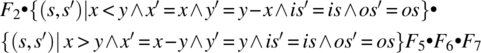
where we use the dot to designate concatenation. Lines 3 and 5 have the same code: hence they compute the same function, which is:
As for line 4, it computes the following function:
Finally, line 6 computes a subset of identity, as follows:
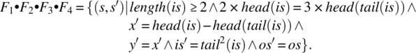
Computing the product F2 • F3 • F4 • F5 • F6 • F7, we find:
= {associativity, substitution}
= {relational product}
= {associativity, substitution}

= {relational product}

= {associativity, substitution (post-restriction)}

= {simplification, assumption that x and y are both positive}
= {relational product, abbreviating each function by its initial}
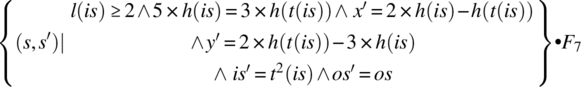
= {relational product}
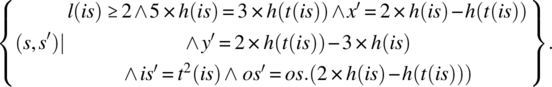
This function reflects the impact of the path on the state variables; remember that l(is), h(is), and h(t(is)) are (respectively) the length, first element, and second element of the input stream. Note that if the first element is 18 and the second element is 30, then upon execution of this path, the input stream is truncated by two, and the output stream is augmented by a new element, whose value is: 2 × 18 − 30 = 6. Indeed, 6 is the greatest common divisor of 18 and 30.
Before we close this section, we give a useful rule on how to compute the product of two functions that are written in the following form (on some space S defined by two variables x and y):
Let functions F1 and F2 be written as:
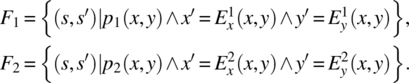
Then the product of functions F1 and F2 is given by the following formula:
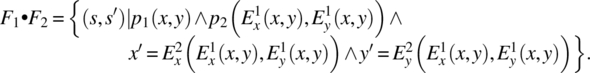
As an illustration, consider the following functions on a space S defined by integer variables x and y:
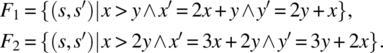
Then the product of these two functions yields the following result:
After simplification, we find:
The product of two functions takes a special, simpler, form whenever one of the factors is a subset of the identity; specifically, we have

and

In order to spare the reader the trouble of having to refer to the definition whenever he/she must compute the product of two functions, we present below a set of rules that streamline this process.
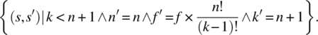
As an illustration of this formula, we consider the product of the following functions on space S defined by natural variables n, f, and k:
-
 .
. -
 .
.
Applying the proposed formula, we find the following relation:
= {proposed formula}

= {merging the preconditions, simplifying}
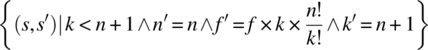
= {because ![]() !}
!}
10.1.3 Path Conditions
The condition of a path is the condition that an initial state must satisfy in order for that path to be taken during an execution of the program. As an illustrative example, we consider path p8, and we find that its path condition is:
We let the first and second elements of the input stream is be, respectively, 18 and 30; they clearly satisfy the path condition of path p8, since ![]() . We draw a flowchart of program p and analyze what path the execution of this program follows for the selected values.
. We draw a flowchart of program p and analyze what path the execution of this program follows for the selected values.
| statement | is | os | x | y | (x!=y) | (x>y) |
| (18, 30, ..) | (..) | |||||
| int x; int y; | (18, 30, ..) | (..) | ? | ? | N/A | N/A |
| read(x); | (30, ..) | (..) | 18 | ? | N/A | N/A |
| read(y); | (..) | (..) | 18 | 30 | N/A | N/A |
| while (x!=0) | (..) | (..) | 18 | 30 | True | N/A |
| if (x>y) | (..) | (..) | 18 | 30 | N/A | False |
| y=y-x | (..) | (..) | 18 | 12 | N/A | N/A |
| while (x!=0) | (..) | (..) | 18 | 12 | True | N/A |
| if (x>y) | (..) | (..) | 18 | 12 | N/A | True |
| x=x-y | (..) | (..) | 6 | 12 | N/A | N/A |
| while (x!=0) | (..) | (..) | 6 | 12 | True | N/A |
| if (x>y) | (..) | (..) | 6 | 12 | N/A | False |
| y=y-x | (..) | (..) | 6 | 6 | N/A | N/A |
| while (x!=0) | (..) | (..) | 6 | 6 | False | N/A |
| Write(x); | (..) | (..).6 | 6 | 6 | N/A | N/A |
The reader can see that the sequence of statements in the first column of the table above does indeed correspond to path p8 (Fig. 10.1).
Figure 10.1 Flowchart of a GCD program.
The ability to represent paths, compute their function, and their path condition, will all be useful in the remainder of this chapter as we explore criteria for generating test data.
10.2 CONTROL FLOW COVERAGE
Control flow coverage criteria provide for generating sufficient test data to exercise various features of the control structure of candidate programs.
10.2.1 Statement Coverage
The statement coverage criterion provides for generating sufficient test data to execute each statement of the candidate program at least once. This is a very weak criterion, since the only faults it is likely to expose are those that are so egregious that any execution of the faulty statement will cause an error, and that the error is so extensive that it will propagate and cause a failure; by statement, this criterion usually refers to elementary statements, typically assignment statements and atomic system calls. This criterion can also be applied at a higher level of abstraction than the elementary statement, and calls for exercising all the components of a composite system, with the same qualification: it can only expose faulty components that are so egregiously faulty that any execution of these components will sensitize their fault and subsequently propagate the resulting error to cause failure. Because this criterion is so weak, a single path may, conceivably, satisfy it, in some simple cases.
As an illustration, we consider the following simple program g:
{int x; int y; read(x); read(y); // assuming x>0, y>0while (x!=y) {if (x>y) {x=x-y;} else {y=y-x;}};write(x);}
Execution of the following path through the program will exercise all the elementary statements:
p: int x; int y;// F0
  read(x); read(y);// F1
    ((x!=y)? true); ((x>y)? true); {x=x-y;}// F2
    ((x!=y)? true); ((x>y)? false); {y=y-x;}// F3
    ((x!=y)? false);// F4
    {write(x);// F5
The effect of F0 is to let the space of the program be defined by variables is and os of type file stream and variables x and y of type integer; all subsequent functions will be defined on this space. We find:
The product of F2 by F3 yields:
Whence, the product of F2 • F3 by F4 yields:
which we simplify to become:
Multiplying on the left by F1, we find
Multiplying on the right by F5, we find
The domain of this function is:
Any element of this domain is a possible test data that satisfies the criterion of statement coverage; we choose the initial state s defined by:
Even though a single path (and a single element in the domain of the path) enabled us to satisfy the criterion of statement coverage, it may be beneficial, in practice, to cover different statements with different paths (whenever possible) to minimize the likelihood of error masking (the longer the path, the more likely it is for an error to be masked). To this effect, we may satisfy the statement coverage with the following two paths:
p1: int x; int y;// F0
   read(x); read(y);// F1
   ((x!=y)? true); ((x>y)? true); {x=x-y;}// F2
   ((x!=y)? false);// F3
   {write(x);// F4
p2: int x; int y;// F0
   read(x); read(y);// F1
   ((x!=y)? true); ((x>y)? false); {y=y-x;}// F2
   ((x!=y)? false);// F3
   {write(x);// F4
We leave it as an exercise to the reader to generate test data from these two paths.
10.2.2 Branch Coverage
The criterion of branch coverage provides that we generate test data so that for each branch in the control structure of the candidate program (whether it arises in an if-then statement, an if-then-else statement, or a while statement), the program proceeds through each of the True branch and the False branch at least once. As an illustration of this criterion, we consider the following program:
#include <iostream>#include <cmath>using namespace std;/* constants */float eps = 0.000001;/* state variables */float x, y, z;/* functions */Bool tri(float x, float y, float z);bool equal(float a, float b);bool equi(float x, float y, float z);bool iso(float x, float y, float z);bool right(float x, float y, float z);int main (){cout << “enter the triangle sides on one line” << endl;cin >> x >> y >> z;if (!tri(x,y,z)){cout << “not a triangle” << endl;}else{if (equi(x,y,z)){cout << “equilateral” << endl;}elseif (iso(x,y,z)){if (right(x,y,z)) {cout << “isoceles right” << endl;}else {cout << “isoceles” <<endl;}else{if (right(x,y,z)) {cout << “right” << endl;}else {cout << “scalene” << endl;}}}}bool tri (float x, float y, float z){return ((x<=y+z) && (y<=x+z) && (z<=x+y));}bool equal (float a, float b){return abs(a-b)<eps;}bool equi(float x, float y, float z){return (equal(x,y) && equal(y,z));}bool iso(float x, float y, float z){return (equal(x,y) || equal(y,z) || equal(x,z));}bool right(float x, float y, float z){return (equal(x*x+y*y,z*z) || equal(x*x+z*z,y*y) || equal(y*y+z*z,x*x));}
The following set of paths allows us to traverse every branch at least once:
-
p1: cout << “enter the triangle sides on one line” << endl;
   cin >> x >> y >> z;
((!tri(x,y,z))? True) {cout << “not a triangle” << endl;} -
p2: cout << “enter the triangle sides on one line” << endl;
   cin >> x >> y >> z;
((!tri(x,y,z))? False);((equi(x,y,z))? True)
{cout << “equilateral” << endl;} -
p3: cout << “enter the triangle sides on one line” << endl;
   cin >> x >> y >> z;
   ((!tri(x,y,z))? False); ((equi(x,y,z))? False);
   ((iso(x,y,z))? True); ((right(x,y,z))? True);
{cout << “isoceles right” << endl;} -
p4: cout << “enter the triangle sides on one line” << endl;
   cin >> x >> y >> z;
   ((!tri(x,y,z))? False); ((equi(x,y,z))? False);
   ((iso(x,y,z))? True); ((right(x,y,z))? False);
{cout << “isoceles” << endl;} -
p5: cout << “enter the triangle sides on one line” << endl;
   cin >> x >> y >> z;
   ((!tri(x,y,z))? False); ((equi(x,y,z))? False);
   ((iso(x,y,z))? False); ((right(x,y,z))? True);
{cout << “right” << endl;} -
p6: cout << “enter the triangle sides on one line” << endl;
   cin >> x >> y >> z;
((!tri(x,y,z))? False); ((equi(x,y,z))? False);
((iso(x,y,z))? False); ((right(x,y,z))? False);
{cout << “scalene” << endl;}
A brief inspection of the paths presented above enables us to check that each condition appears at least once with the outcome True and once with the outcome False. In the following table, we list the paths, along with their path conditions and a test vector that satisfies the path condition.
| Path | Path condition | Test vector |
p1 |
((!tri(x,y,z))? True) |
2 2 10 |
p2 |
((!tri(x,y,z))? False); ((equi(x,y,z))? True) |
2 2 2 |
p3 |
((!tri(x,y,z))? False); ((equi(x,y,z))? False);
((iso(x,y,z))? True); ((right(x,y,z))? True); |
2 2 |
p4 |
((!tri(x,y,z))? False); ((equi(x,y,z))? False);
((iso(x,y,z))? True); ((right(x,y,z))? False); |
2 2 1 |
p5 |
((!tri(x,y,z))? False); ((equi(x,y,z))? False);
((iso(x,y,z))? False); ((right(x,y,z))? True); |
3 4 5 |
p6 |
((!tri(x,y,z))? False); ((equi(x,y,z))? False);
((iso(x,y,z))? False); ((right(x,y,z))? False); |
3 4 6 |
10.2.3 Condition Coverage
A variation of the previous criterion can be applied for programs that have compound conditions and it provides for generating test data to let each term of any condition (rather than the condition as a whole) take both truth values, true and false. So that if the condition has the form
it is not enough to let the condition be true then false, but we want to ensure that each individual term takes both truth values through the test. To generate test data according to this criterion, we proceed as follows:
As an illustration, we consider the following triangle program, which we modify specifically to create compound conditions.
#include <iostream>#include <cmath>using namespace std;/* constants */float eps = 0.000001;/* state variables */float x, y, z;/* functions */bool tri(float x, float y, float z); // trianglebool equal(float a, float b); // equal, within epsbool equi(float x, float y, float z); // equilateralbool iso(float x, float y, float z); // isocelesbool right(float x, float y, float z); // right triangleint main () {cout << “enter the triangle sides on one line”<< endl;cin >> x >> y >> z;if (!tri(x,y,z)) {cout << “not a triangle” << endl;}if (tri(x,y,z) && equi(x,y,z)) {cout << “equilateral” << endl;}if (tri(x,y,z) && (!equi(x,y,z)) && iso(x,y,z) && (!right(x,y,z))){cout << “isoceles” << endl;}if (tri(x,y,z) && (!equi(x,y,z)) && (!iso(x,y,z)) && right(x,y,z)){cout << “right” << endl;}if (tri(x,y,z) && (!equi(x,y,z)) && iso(x,y,z) && right(x,y,z)){cout << “isoceles right” << endl;}if (tri(x,y,z) && (!equi(x,y,z)) && (!iso(x,y,z)) && (!right(x,y,z))){cout << “scalene” << endl;}}
We can simplify this program by referring to the following identities:
- An equilateral triangle is isosceles; hence a non-isosceles triangle is not equilateral.
- A triplet (x, y, z) that satisfies right(x, y, z) necessarily satisfies tri(x, y, z).
- A triplet (x, y, z) that satisfies equi(x, y, z) necessarily satisfiestri(x, y, z).
We find:
int main () {cout << “enter the triangle sides on one line” << endl;cin >> x >> y >> z;if (!tri(x,y,z)) {cout << “not a triangle” << endl;}if (equi(x,y,z)) {cout << “equilateral” << endl;}if (tri(x,y,z) && (!equi(x,y,z)) && iso(x,y,z) && (!right(x,y,z))){cout << “isoceles” << endl;}if ((!iso(x,y,z)) && right(x,y,z)) {cout << “right” << endl;}if ((!equi(x,y,z)) && iso(x,y,z) && right(x,y,z)){cout << “isoceles right” << endl;}if (tri(x,y,z) && (!iso(x,y,z)) && (!right(x,y,z))){cout << “scalene” << endl;}}
In this particular example, all the if-statements refer to the same values of variables x, y, and z. Indeed, though they are written sequentially, the if-statements are merely printing messages to the output stream and are not altering the program variables that are invoked in the conditions. A cursory inspection of the structure of the conditions reveals that the criterion of condition coverage is satisfied if we generated test data to ensure that each elementary function call returns both truth values, in turn. The following table shows sample test data that satisfies this criterion.
| Condition | True | False |
tri(x,y,z) |
5 6 7 | 5 6 12 |
equi(x,y,z) |
6 6 6 | 6 7 6 |
iso(x,y,z) |
5 5 12 | 5 7 6 |
right(x,y,z) |
3 4 5 | 3 4 6 |
Note that the data generated to make iso(x, y, z) true does not define a triangle, nor does it have to—it only has to make iso(x, y, z) true; such data will cause the program to declare that the data entered does not define a triangle.
10.2.4 Path Coverage
The criterion of path coverage provides that we generate test data to exercise every execution path of candidate programs. If the program has no loops, then the set of paths is finite, and can be easily catalogued; to get a sense of the work involved in this task, we consider the two versions of the triangle analysis program (the nested version and the sequential version). The flow chart of the nested version looks as follows (Fig. 10.2).
Figure 10.2 Flowchart of a Triangle program: nested version.
Figure 10.3 Flowchart of a Triangle program: sequential version.
Paths in the program correspond to paths from the first node to the exit node in this graph; covering all the paths corresponds, in this case, to branch coverage. We characterize each path by the sequence of conditions that it evaluates as it proceeds from the start to the exit node, and we find the following paths.
| Path | Condition | Test Data | ||||
| x | y | z | ||||
| p1 | !tri() |
2 | 4 | 8 | ||
| p2 | tri()&& equi() |
2 | 2 | 2 | ||
| p3 | tri() && !equi() && iso() && right() |
1 | 1 | |||
| p4 | tri()&& !equi() && iso() && !right() |
4 | 4 | 3 | ||
| p5 | tri() && !equi() && !iso() && right() |
3 | 4 | 5 | ||
| p6 | tri() && !equi() && !iso() && !right() |
2 | 3 | 4 | ||
We consider now the sequential version of the triangle analysis program (Fig. 10.3). Topologically, this flowchart appears to have 26 paths, since it has six binary conditions in sequence; but in fact many of these paths are not executable (their path function is empty) due to the dependencies between the conditions. If we identify each path by the sequence of True/False (T/F) values of the conditions, we find the following paths:
| Path | !tri | equi |
tri && !equi && iso && !right | !iso && right | !equi && iso && right | tri && !iso && !right |
| p1 | T | F | F | F | F | F |
| p2 | F | T | F | F | F | F |
| p3 | F | F | T | F | F | F |
| p4 | F | F | F | T | F | F |
| p5 | F | F | F | F | T | F |
| p6 | F | F | F | F | F | T |
Notice that in this table, each row is fully determined by the shaded area. For example, in the first row (path p1), consider that if condition (!tri) returns True, then all subsequent expressions necessarily return False: for example, the second column (condition: equi) returns False since a set of three identical numbers define a triangle; the third column (condition: tri && !equi && iso && !right) returns False since the first conjunct (tri) is already known to be False; etc. Hence the paths p1, p2, p3, p4, p5, p6 presented in this table are the only feasible paths (out of 26) of the program. The following table characterizes each one of these paths and proposes a data item that falls in their domain.
| Path | Path Condition | Test Data |
| p1 | !tri | 2 4 10 |
| p2 | equi |
3 3 3 |
| p3 | tri && !equi && iso && !right | 3 3 4 |
| p4 | !iso && right | 3 4 5 |
| p5 | !equi && iso && right | 3 3 3 |
| p6 | tri && !iso && !right | 4 5 6 |
The sample examples we have studied so far have a finite number of paths, since they have no iterative statements; with while loops, we face the possibility of having an infinite number of paths; for such cases the criterion of path coverage cannot be fulfilled to the letter. We resort to approximations of this criterion, whereby we consider upper bounds on the number of iterations for each loop. Because we may have nested loops, even this approximate criterion may cause a combinatorial explosion, producing up to Np paths, where N is the upper bound on the number of iterations and p is the depth of nesting of the loops.
As an example, we consider the gcd program discussed in Section 10.1:
{int x; int y; read(x); read(y); // assuming x>0, y>0while (x!=y) {if (x>y) {x=x-y;} else {y=y-x;}};write(x);}
We resolve to apply the path coverage criterion to it, up to three iterations of the while loop. We find the following paths, classified according to the number of iterations:
- Path with Zero iterations:
-
p0: int x; int y; read(x); read(y);
   ((x!=y)? false); write(x);
-
- Paths with One iteration:
-
p11: int x; int y; read(x); read(y);
      ((x!=y)? true); ((x>y)? true); x=x-y;
((x!=y)? false); write(x); -
p12: int x; int y; read(x); read(y);
      ((x!=y)? true); ((x>y)? false); y=y-x;
      ((x!=y)? false); write(x);
-
- Paths with Two iterations:
-
p21: int x; int y; read(x); read(y);
      ((x!=y)? true); ((x>y)? true); x=x-y;
      ((x!=y)? true); ((x>y)? true); x=x-y;
((x!=y)? false); write(x); -
p22: int x; int y; read(x); read(y);
      ((x!=y)? true); ((x>y)? false); y=y-x;
      ((x!=y)? true); ((x>y)? false); y=y-x;
((x!=y)? false); write(x); -
p23: int x; int y; read(x); read(y);
      ((x!=y)? true); ((x>y)? true); x=x-y;
      ((x!=y)? true); ((x>y)? false); y=y-x;
((x!=y)? false); write(x); -
p24: int x; int y; read(x); read(y);
      ((x!=y)? true); ((x>y)? false); y=y-x;
      ((x!=y)? true); ((x>y)? true); x=x-y;
      ((x!=y)? false); write(x);
-
- Paths with Three iterations: In order to keep combinatorics under control, and because x and y play symmetric roles, we do not show all eight paths; but rather only four; the missing four can be retrieved by interchanging x and y.
-
p31: int x; int y; read(x); read(y);
      ((x!=y)? true); ((x>y)? true); x=x-y;
      ((x!=y)? true); ((x>y)? true); x=x-y;
      ((x!=y)? true); ((x>y)? true); x=x-y;
((x!=y)? false); write(x); -
p32: int x; int y; read(x); read(y);
      ((x!=y)? true); ((x>y)? true); x=x-y;
      ((x!=y)? true); ((x>y)? true); x=x-y;
      ((x!=y)? true); ((x>y)? false); y=y-x;
((x!=y)? false); write(x); -
p33: int x; int y; read(x); read(y);
      ((x!=y)? true); ((x>y)? true); x=x-y;
      ((x!=y)? true); ((x>y)? false); y=y-x;
      ((x!=y)? true); ((x>y)? true); x=x-y;
((x!=y)? false); write(x); -
p34: int x; int y; read(x); read(y);
      ((x!=y)? true); ((x>y)? true); x=x-y;
      ((x!=y)? true); ((x>y)? false); y=y-x; ;
      ((x!=y)? true); ((x>y)? false); y=y-x;
      ((x!=y)? false); write(x);
-
We leave it as an exercise to the reader to compute the path functions and the path conditions of these paths; we show the results in the table below, along with test data that meets the path conditions.
| Number of iterations | Path | Condition | Test data | ||||
| x | y | ||||||
| 0 | p0 | x=y | 5 | 5 | |||
| 1 | p11 | x=2y | 10 | 5 | |||
| p12 | y=2x | 5 | 10 | ||||
| 2 | p21 | x=3y | 15 | 5 | |||
| p22 | y=3x | 5 | 15 | ||||
| p23 | 2x=3y | 15 | 10 | ||||
| p24 | 3x=2y | 10 | 15 | ||||
| 3 | p31 | x=4y | 20 | 5 | |||
| p32 | 2x=5y | 25 | 10 | ||||
| p33 | 3x=5y | 15 | 9 | ||||
| p34 | 3x=4y | 16 | 12 | ||||
The test data for the four missing paths resulting from three iterations can be computed by merely interchanging x and y in the test data of the paths of length 3; we find,
| Number of iterations | Path | Condition | Test data | ||||
| x | y | ||||||
| 3 | p31 | y=4x | 5 | 20 | |||
| p32 | 2y=5x | 10 | 25 | ||||
| p33 | 3y=5x | 9 | 15 | ||||
| p34 | 3y=4x | 12 | 16 | ||||
10.3 DATA FLOW COVERAGE
Whereas in the previous section we explored how to generate test data by analyzing the control flow of candidate programs in execution, in this section we explore how we can use the data flow of the program as a guide to generate adequate test data.
10.3.1 Definitions and Uses
The life of a program variable during the execution of a program lasts from the time the variable becomes known as part of the program state to the time it is no longer accessible to the program as part of the state. Under static block-structured dynamic allocation, the name of a variable is known from the time of its declaration to the time when execution of the program exists the block where it is declared; under dynamic memory allocation, the name of a variable is known between the time the program creates the variable through an instantiation (by means of a new statement), and the time when the program explicitly returns the name (implicitly relinquishing the memory space to which it refers) or terminates its execution. Several relevant events arise during the lifecycle of a variable, including:
- Assignment of a value to the variable, through an assignment statement, or through a read statement, or at instantiation time through invocation of the constructor method of a class, or at declaration time through compiler-generated initializations, or through parameter passing of the variable as a reference parameter to a routine. We refer to these events as definitions of the variable.
- Use of the value of the variable, to compute an expression, or through a write statement, or in a branch condition, or as an index to an array, or through parameter passing of the variable as a value parameter to a routine. We refer to these events as uses of the variable, and we distinguish between
- c-uses, when the variable is used to compute an expression and
- p-uses, when the variable is used to compute a Boolean condition that affects the program control.
Notice that the same variable may be considered c-used and p-used if it intervenes in an expression to compute a Boolean condition; such is the case, for example, for variable x in the following Boolean condition:
if ((x+2)>0) {…;}Notice also that in a statement such as
a[i]=x+3;for example, we consider that a is defined, i is c-used (even though it is used to compute an address/a location rather than a value), and x is c-used; strictly speaking, this statement only defines the ith cell of array a, but since we cannot identify the exact cell that has been modified, we assume that all of a has been (re-) defined.
- Termination of the lifecycle of the variable, when the variable is no longer part of the state of the program, either because control has exited the block where it was declared (in block structured programs) or because it has been explicitly relinquished (as is the case with some dynamic allocation schemes) or the program terminates its execution.
As an illustration of definitions and uses, we consider the gcd program, which handles integer (natural) variables x and y:
{int x; int y;// 1read(x);// 2read(y);// 3while (x!=y)// 4{if (x>y)// 5{x=x-y;}// 6else// 7{y=y-x;}};// 8write(x);// 9}// 10
The following table shows for each variable the statements in which the variable is defined, c-used, p-used, and terminated.
| Line | x | y | ||||||
| Defined | c-used | p-used | Terminated | Defined | c-used | p-used | Terminated | |
| 1 | ||||||||
| 2 | √ | |||||||
| 3 | √ | |||||||
| 4 | √ | √ | ||||||
| 5 | √ | √ | ||||||
| 6 | √ | √ | √ | |||||
| 7 | ||||||||
| 8 | √ | √ | √ | |||||
| 9 | √ | |||||||
| 10 | √ | √ | ||||||
We can write the lifecycle of each variable as follows, by indicating the sequence of events that arose in the lifecycle, along with the lines where they did:
- Variable x: defined(2); p-used(4); p-used(5); c-used(6); defined(6); c-used(8); terminated(10).
- Variable y: defined(3); p-used(4); p-used(5); c-used(6); c-used(8); defined(8); terminated(10).
If we observe a program in execution and focus on the sequence of events that take place during the lifecycle of any variable, we may find that some patterns are outright wrong, and some patterns, while they may be correct, look suspicious nevertheless, hence may deserve extra scrutiny. Among incorrect event sequences, we cite the following:
- A variable that is used (use, c-use, p-use) before being defined (without being assigned a value).
- A variable that is used after its termination.
As for suspicious patterns, we cite the following instances:
- A variable that is defined twice in sequence without being used in the intervening time.
- A variable that is defined and then killed without being reused.
These patterns do not necessarily indicate the presence of a fault, but they do warrant careful consideration. For strictly sequential programs, it is possible for the compiler to detect incorrect patterns and suspicious patterns; but with control structures such as if-then statements, if-then-else statements and loops, the compiler cannot predict execution sequences at compile time. The goal of data flow test generation criteria is to generate test data in such a way as to execute all the paths that may have incorrect or suspicious event sequences; we review a sample of these criteria in the following sections.
10.3.2 Test Generation Criteria
The purpose of dataflow-based test generation criteria is to force the execution of the program through combinations of definitions and uses in such a way as to detect all possible faults in the sequencing of these events. We discuss four such criteria:
- All definition-use paths. A path in the program is said to be a definition-use path (du-paths, for short) for some program variable x if and only if it starts with some statement that defines variable x and ends with a statement that uses variable x.
- All definition-clear paths. A path in the program is said to be a definition-clear path for some program variable x if and only if it is a definition-use path for variable x and the definition statement with which it starts is the only definition statement for that variable in the path.
The criterion of All definition-use paths provides that one must generate test data to exercise all the definition-use paths for all the variables of the program. To apply this criterion, we proceed as follows:
- First, we list all the variables of the program.
- For each variable of the program, we list all the definition statements and all the use statements.
- For each definition/use pair, we check whether there exists a path from the definition statement to the use statement.
- For all the paths identified in the previous steps, we identify a pre-path, from the beginning of the execution to the first statement of the path, and a post-path, from the last statement of the path to the end of the execution.
- For each triplet made up of a pre-path, a definition-use path, and a post-path, we compute the function of the aggregate path.
- For each aggregate path, we compute the path condition as the domain of the path function.
- For each path that yields a non-False path condition, we generate test data that exercises this path.
- All definition-clear paths. A path in the program is said to be a definition-clear path for some program variable x if and only if it is a definition-use path for variable x and the definition statement with which it starts is the only definition statement for that variable in the path.
The set of test data so obtained constitutes our test data.
- All p-uses. A p-use path for a program with respect to variable x is a definition-clear path from a definition of variable x to a p-use of x. The criterion of All p-uses provides that one must generate test data to exercise all the p-use paths for all the variables of the program. To apply this criterion, we proceed in the same way as we discuss above, but focusing exclusively on p-use paths.
- All c-uses. A c-use path for a program with respect to variable x is a definition-clear path from a definition of variable x to a c-use of x. The criterion of All c-uses provides that one must generate test data to exercise all the c-use paths for all the variables of the program. To apply this criterion, we proceed in the same way as we discuss above, but focusing exclusively on c-use paths.
- All uses. The criterion of All uses provides that one must generate test data to meet the All p-uses criterion and test data to meet the All c-uses criterion.
- All definitions. The criterion of All definitions provides that one must generate test data to ensure that all definitions are visited at least once.
For the sake of illustration, we briefly discuss the generation of test data according to the four criteria presented herein for the gcd program. We apply the criteria in turn, below:
- All du-paths. We consider in turn variable x, then variable y. For variable x, we find the following definition statements:
-
Statements 2 and 6.
And the following use statements:
- Statements 4, 5, 6, 8, and 9.
-
Statements 2 and 6.
We choose the definition-use path that starts at the definition in statement 2 and ends at the use at statement 4. We write this path as follows:
read(x); read(y); ((x!=y)? XX);
The pre-path of this path is empty, since read(x) is the first executable statement of the program. There is an infinity of post-paths; for the sake of illustrations, we do not take the shortest/simplest post-path, but choose instead the following:
((x!=y)? true); ((x>y)? true); (x=x-y); ((x>y)? false); write(x);
We leave it to the reader to check that the function of this path is the following:
The domain of this function can be written as:
Possible test data:
We leave it to the interested reader to continue reviewing other definition-use paths, including those obtained by the combinations of statements (2,5), (2,6), (2,8), (6,4), (6,5), and (6,8). Note that by the time we combine the selected path with a pre-path and a post-path, we may find an aggregate path that we have analyzed before; in that case, we can rely on the test data we have generated before.
We must do the same analysis for all the definition-use paths that pertain to variable y; to this effect, we list below the definition and use statements for variable y.
- Definitions: statements 3 and 8.
- Uses: statements 4, 5, 6, 8.
- All p-uses. This criterion provides for covering all the definition-clear paths that end with a p-use of some variable. The following table shows the list of definitions and p-uses of each variable of the program.
This includes definition-clear paths (2,4), (2,5), (3,4), and (3,5).
x y Definitions 2, 6 3, 8 p-uses 4, 5 4, 5 - All c-uses. This criterion provides for covering all the definition-clear paths that end with a c-use of some variable. The following table shows the list of definitions and p-uses of each variable of the program.
This includes definition-clear paths (2,6), (6,8), (3,8).
x y Definitions 2, 6 3, 8 c-uses 6, 8 6, 8 - All uses. The test data generated for this criterion is the union of the test data generated by criterion All p-uses and criterion All c-uses.
- All definitions. The test data generated for this criterion must ensure that all the definition nodes are visited at least once; these are 2 and 6 for x, and 3 and 8 for y.
10.3.3 A Hierarchy of Criteria
A test data generation criterion C subsumes a test data generation criterion C′ if and only if any test data set that satisfies C satisfies C′. The following subsumption relations hold between the criteria discussed in this section (Fig. 10.4).
Figure 10.4 Hierarchy of test generation criteria.
10.4 FAULT-BASED TEST GENERATION
Whereas the previous sections focus on generating test data to cover the control flow and the data flow of the program, this section focuses on generating test data to expose specific types of faults, namely faults in Boolean conditions in the program. We distinguish between the following types of faults in Boolean expressions and conditions:
- Variable Reference Fault, where a Boolean variable is replaced by another.
- Variable Negation Fault, where a Boolean variable is replaced by its negation.
- Expression Negation Fault, where a Boolean expression is replaced by its negation.
- Associative Shift Fault, where a Boolean expression is parenthesized incorrectly; for example, the expression
 is written instead of
  .
. - Operator Reference Fault, where the wrong Boolean operator is used in an expression; for example, the expression
 is written instead of
  .
. - Relational Operator Fault, where the wrong relational operator is used in a Boolean valued expression; for example, the expression
 is used instead of
  .
.
In this section, we discuss how we can generate test data to expose such faults, if they arise in Boolean conditions and Boolean expressions of a candidate program. To do so, we proceed in three steps:
- First, for each type of fault, we want to characterize the local data that sensitizes the fault, and converts it into an error.
- Second, we want to characterize the input data that generates the necessary local conditions for the fault to be sensitized.
- Third, we want to further refine the data selection criterion to ensure that, in addition to generating an error, the data will also propagate the error to lead to an observable failure.
We review these three conditions in the following sections.
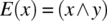
10.4.1 Sensitizing Faults
Let E be a Boolean expression in a program; we assume that E has one of the faults classified above, and we let E′ be the Boolean expression obtained from E by correcting the fault in question. For example, let E be the Boolean expression ![]() and let there be a variable reference fault in E with respect to variable y (which should have been z, say), then E′ is
and let there be a variable reference fault in E with respect to variable y (which should have been z, say), then E′ is ![]() . We are interested to determine under what condition (on program variables x, y, and z) can this fault be sensitized. In order for expression E to be different from expression E′, the following condition has to hold:
. We are interested to determine under what condition (on program variables x, y, and z) can this fault be sensitized. In order for expression E to be different from expression E′, the following condition has to hold:
where ⊕ represents the operator of exclusive or: ![]() . This expression is true if and only if the Boolean values of expressions E and E′ are distinct (one is True, the other is False). To understand the meaning of this condition, consider the following simple example:
. This expression is true if and only if the Boolean values of expressions E and E′ are distinct (one is True, the other is False). To understand the meaning of this condition, consider the following simple example:
-
 .
. -
 .
.
We find,
= {Substitution, expansion}
= {DeMorgan}
= {Distributivity, simplification}
= {Factoring, Definition of ![]() }
}
Indeed, if expression E is faulty and expression E′ is the correct expression, then the only way to sensitize this fault is to let x be true and let y be different from z. As long as y and z take the same values, we will never know that we are referring to the wrong variable (y rather than z); also, as long as x is false, the value of the expression is false regardless of whether the second term is y or z. Hence the condition ![]() is indeed the condition under which the fault can be sensitized and produce an error.
is indeed the condition under which the fault can be sensitized and produce an error.
We review in turn all the classes of faults catalogued above and discuss what form the condition of fault sensitization has for them.
- Variable Reference Fault. If expression E(x) depends on variable x and it should be referring to y instead of x, then the condition of sensitization is:An example of such a situation is given above.

- Variable Negation Fault. If expression E(x) depends on variable x and it should be referring to
 instead of x, then the condition of sensitization is:As an illustrative example, we consider expression E(x) defined as:
 and we assume that the reference to x should have been negated, hence
 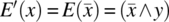 , then the condition of sensitization is:
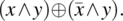
We analyze this expression, as follows:
= {Expanding}

= {De Morgan}
= {Distribution, cancellation}
= {Simplification}

Clearly, the only way to sensitize this fault is to let y be true, since if y were false then the expression would be false regardless of the value of x. Whereas with y at true, the expression would be equal to x and hence reflects whether we have the right value or its negation.
- Expression Negation Fault. If the faulty expression is the negation of the fault-free expression, then any evaluation of the expression sensitizes the fault. Indeed, we have, by definitionfor all expression E.
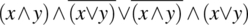
- Associative Shift Fault. This fault arises when a Boolean expression is parenthesized wrong. As an illustrative example, we consider the following expression
 and we assume that the fault free expression is
 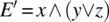 . We analyze the expression
  to determine under what condition this fault may be sensitized; rather than doing this algebraically (using logic identities), we use truth tables to compute the two expressions and then characterize the rows for which the two expressions are distinct:
Hence this condition can be simplified into
to determine under what condition this fault may be sensitized; rather than doing this algebraically (using logic identities), we use truth tables to compute the two expressions and then characterize the rows for which the two expressions are distinct:
Hence this condition can be simplified intox y z 

E E′ 
F F F F F F F F F F T F T T F T F T F F T F F F F T T F T T F T T F F F F F F F T F T F T T T F T T F T T T T F T T T T T T T F  . Indeed, if z is True and x is False, then
  regardless of the value of y and
  regardless of the value of y.
 - Operator Reference Fault. We let E be the original expression and E′ be the corrected expression, and we compute/analyze the expression
 . For example, if we let E be the expression
  and E′ be the expression
  , then we find:= {substitution, expansion}
= {De Morgan}

= {Distributing, simplifying}

= {Definition}

In other words, in order to sensitize this fault, we must submit distinct values for x and y ((true, false) or (false, true)); indeed, if x and y are identical, then their conjunction (∧) and their disjunction (∨) are identical.
- Relational Operator Fault. If a relational operator is faulty, then we need to proceed in two steps: first, we choose data that yields different Boolean values for the relational expression; then we treat the relational expression as a variable reference fault. For example, let i and j be integer variables and let x be a Boolean variable (or another Boolean valued expression). We let expressions E and E’ be defined as follows:
-
 ,
, -
 .
.
 logically implies
  , the only way to make these conditions distinct is to let the first condition be false while the second is true. To this effect, we let i and j be equal. From then on, the question is how to make an expression (x∧y) distinct from (x∧z) given that y is different from z. We have seen in the study of the first class of fault that this requires the condition
  . Since
  is true by construction, the remaining condition for us is x.
 -
All the sensitization conditions we have generated so far are local conditions, that is. conditions that refer to the value of program variables at the state where the Boolean expressions are evaluated; but generating test data requires that we compute conditions that input data must satisfy. In the following section, we consider how to generate test data that triggers sensitization conditions at chosen locations in the program, where the targeted Boolean conditions are evaluated.
10.4.2 Selecting Input Data for Fault Sensitization
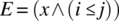
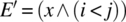
For the sake of this discussion, we introduce a program label that indicates the first executable statement of the program, and we refer to it as the begin label. Also, we consider a Boolean expression E and designate the program label where this expression is evaluated by L. We consider a possible fault in expression E (among the classes of faults catalogued in Section 10.4.1) and we let E′ be the expression obtained from E when the fault is removed; also, we let C be the sensitization condition of the targeted fault at E, that is, ![]() . We have the following criterion:
. We have the following criterion:
As an illustrative example, we consider an array a of size ![]() for some natural number N greater than 1 and an element x of the same data type as the contents of the array; we assume that we are interested in checking whether x is in the first half of the array. Hence we write the following program:
for some natural number N greater than 1 and an element x of the same data type as the contents of the array; we assume that we are interested in checking whether x is in the first half of the array. Hence we write the following program:
void main (){itemtype a[2*N]; itemtype x; indextype i; bool found;i=0; L: while ((a[i]!=x) && (i<=N)) {i=i+1;}found = (a[i-1]==x);}
We have a relational operator fault in this program, as the loop condition should read ((a[i]!=x) && (i<N)) rather than ((a[i]!=x) && (i<=N)). As we discuss in the previous section, this fault can be sensitized locally by ensuring that (i<=N) holds while (i<N) does not, and ensuring that (a[i]!=x)is true. To this effect, we let i be equal to N while ensuring that the condition (a[N]!=x) is true. We write the local sensitization condition as:
All these are local conditions; we must now determine what input data will create these local conditions at label L? To this effect, we compute a path from the start of the program to label L, take its post-restriction to the sensitization condition, check that it is nonempty, then compute its domain. We find:
Path: i=0; ((((a[i]!=x) && (i<=N))? True) ; {i=i+1})*;
where the * is used to refer to an arbitrary number of instances of a path. The function of this path is given by the following formula (where the star represents reflexive transitive closure):
= {Substitution}
= {Transitive Closure}
= {Relational Product}
= {Simplification}
Taking the post-restriction of this function to the sensitization condition, we find
= {Substitution}
= {Simplification}
The domain of this function is:
Any initial state in this domain will sensitize the fault: Indeed, since the condition ![]() holds for all indices between 0 and N inclusive, the second conjunct of the while condition determines the value of this condition: For i=N, the condition
holds for all indices between 0 and N inclusive, the second conjunct of the while condition determines the value of this condition: For i=N, the condition (i<=N) returns True, whereas the condition (i<N) returns False.
10.4.3 Selecting Input Data for Error Propagation
Whereas it is necessary to identify the conditions under which an initial state sensitizes a fault to create an error, it is not sufficient. We also need to make sure the error propagates to cause an observable failure. Whence the following criterion:
The first condition ensures that the fault is sensitized and the second condition ensures that the resulting error is propagated to cause a failure, which can then be observed to infer the existence of the fault. As an illustration, consider again the search program we had introduced above:
void main (){itemtype a[2*N]; itemtype x; indextype i; bool found;i=0; L: while ((a[i]!=x) && (i<=N)) {i=i+1;}found = (a[i-1]==x);}
If we let g’ be the program obtained from g by changing the condition (i<=N) into the condition (i<N), and we let s be an element of dom(P • I(C)), then we find that application of functions G and G′ to s yield the following results:
- For
 .
. - For
 .
.
Indeed, the images of s by G and G′ are distinct (distinct values of i′); hence the error caused by the identified fault is propagated to cause failure; had program G altered variable i in a non-injective manner, such as (for example):
void main (){itemtype a[2*N]; itemtype x; indextype i; bool found;i=0; L: while ((a[i]!=x) && (i<=N)) {i=i+1;}found = (a[i-1]==x); i=0;}
then state s would no longer be an adequate choice to expose the selected fault, even though it does sensitize the fault and causes an error.
10.5 CHAPTER SUMMARY
Structural criteria for test data generation aim to generate test data not by analyzing the functional specification of the product but rather by analyzing the product itself; while the idea of using a product under test as a guide to test may be counter-intuitive, it does ensure some degree of coverage of the code that we are trying to test. Most criteria used in this chapter involve computing feasible execution paths through the code, then determining their path conditions, that is, for each path the condition under which that path will in effect be taken during an execution; hence the first topic we must address, and the most critical skill we must develop, is the ability to compute path conditions. We use this ability to study a number of test data generation criteria, including the following:
- Control flow criteria, which aim to ensure that we achieve a degree of coverage of control flow configurations.
- Dataflow criteria, which aim to ensure that we achieve a degree of coverage of various configurations of variable lifecycles.
- Fault-based criteria, which aim to ensure that we expose various configurations of specific faults in the code.
Whereas functional criteria focus on exposing possible software failures, structural criteria aim to expose various configurations of faults that may be causing observed failures.
10.6 EXERCISES
- 10.1. Consider the paths p0, p1, p2, and p3 derived on the gcd program of Section 10.1.
- Compute their path function.
- Compute their path condition.
- Derive test data to meet the path condition of each path.
- 10.2. Consider the paths p4, p5, p6, and p7 derived on the gcd program of Section 10.1.
- Compute their path function.
- Compute their path condition.
- Derive test data to meet the path condition of each path.
- 10.3. Generate four paths of the gcd program of Section 10.1 that proceed through the loop four times.
- Compute their path function.
- Compute their path condition.
- Derive test data to meet the path condition of each path.
- How many paths are there that iterate four times through the loop?
- 10.4. Consider the following program, whose goal is to check whether x is located in the second half of array a of size 2×N, where N>1:
void main (){itemtype a[2*N]; itemtype x; indextype i; bool found;i=2*N-1; L: while ((a[i]!=x) && (i>N)) {i=i-1;}found = (a[i+1]==x);}Find test data to sensitize the fault that the second conjunct of the loop condition should be
(i>=N)rather than(i>N). - 10.5. Consider the following program, whose goal is to check whether x is located in the second half of array a of size 2×N, where N>1:
void main (){itemtype a[2*N]; itemtype x; indextype i; bool found;i=2*N-1; L: while ((a[i]!=x) && (i>N)) {i=i-1;}found = (a[i+1]==x); i=N;}Find test data to expose the fault that the second conjunct of the loop condition should be
(i>=N)rather than(i>N). - 10.6. Consider the two paths proposed at the end of Section 10.2.1. Compute their path functions P1 and P2, then the domains of their path functions. Generate test data from them.
- 10.7. Consider the following program on space S defined by natural variables x, y, and z
{z=1;  while (y!=0) {if (y%2==0) {y=y/2; x=x*x}
else {y=y-1; z=z+x;}}}.- Generate the paths of this program that iterate no more than three times through the loop.
- Compute the function of each path and its path condition.
- Generate test data that satisfies the path condition of each path.
- 10.8. Complete test generation (started in Section 10.3.2) for the gcd program according to the criterion of All du-paths.
- 10.9. Complete test generation (started in Section 10.3.2) for the gcd program according to the criterion of All c-uses.
- 10.10. Complete test generation (started in Section 10.3.2) for the gcd program according to the criterion of All p-uses.
- 10.11. Complete test generation (started in Section 10.3.2) for the gcd program according to the criterion of All definitions.
- 10.12. Consider the following program on space S defined by natural variables x, y, and z
   {z=0;  while (y!=0) {if (y%2==0) {y=y/2; x=2*x}
                else {y=y-1; z=z+x;}}}.
Generate test data for this program using the criterion of All du-paths.
- 10.13. Consider the following program on space S defined by natural variables x, y, and z
   {z=0;  while (y!=0) {if (y%2==0) {y=y/2; x=2*x}
                else {y=y-1; z=z+x;}}}.
Generate test data for this program using the criterion of All u-uses.
- 10.14. Consider the following program on space S defined by natural variables x, y, and z
   {z=0;  while (y!=0) {if (y%2==0) {y=y/2; x=2*x}
                else {y=y-1; z=z+x;}}}.
Generate test data for this program using the criterion of All p-uses.
- 10.15. Consider the following program on space S defined by natural variables x, y, and z
   {z=0;  while (y!=0) {if (y%2==0) {y=y/2; x=2*x}
                  else {y=y-1; z=z+x;}}}.
Generate test data for this program using the criterion of All definitions.
- 10.16. Consider the following program on space S defined by natural variables x, y, and z
   {z=1;  while (y!=0) {if (y%2==0) {y=y/2; x=x*x}
                else {y=y-1; z=z*x;}}}.
Generate test data for this program using the criterion of All du-paths.
- 10.17. Consider the following program on space S defined by natural variables x, y, and z
   {z=1;  while (y!=0) {if (y%2==0) {y=y/2; x=x*x}
                else {y=y-1; z=z*x;}}}.
Generate test data for this program using the criterion of All u-uses.
- 10.18. Consider the following program on space S defined by natural variables x, y, and z
   {z=1;  while (y!=0) {if (y%2==0) {y=y/2; x=x*x}
                else {y=y-1; z=z*x;}}}.
Generate test data for this program using the criterion of All p-uses.
- 10.19. Consider the following program on space S defined by natural variables x, y, and z
   {z=1;  while (y!=0) {if (y%2==0) {y=y/2; x=x*x}
                else {y=y-1; z=z*x;}}}.
Generate test data for this program using the criterion of All definitions.
- 10.20. Consider the sequential form of the triangle analysis program discussed in Section 10.2.4. Review the table that characterizes paths p1–p6, and justify the way this table is filled.
- 10.21. Compute the path functions and the path conditions of the paths generated for the gcd program in Section 10.2.4.
- 10.22. Use fault-based test generation to produce test data for the sequential version of the triangle analysis program.
- 10.23. Use fault-based test generation to produce test data for the nested version of the triangle analysis program.
10.7 BIBLIOGRAPHIC NOTES
The discussion of fault-based test data generation uses results given by Kuhn (1999). The discussion of dataflow-based test data generation uses results from Rapps and Weyuker (1985) and Frankl and Weyuker (1988).