
12
Test Driver Design
In Part III, we have explored means to generate test data, and in Chapter 11, we have discussed ways to generate test oracles; in this chapter, we discuss how to compose test data and test oracles to develop a test driver.
12.1 SELECTING A SPECIFICATION
In Chapter 11, we have discussed how to map a specification against which we want to test a program into a test oracle; in this section, we discuss how to choose a specification. One may argue that the question of what specification to test a program against is moot, since we do not get to choose the specification. We argue that while we do not in general have the luxury of deciding what specification we must test a program against, we do have some latitude in choosing how to deploy different verification methods against different components of a complex, compound specification. Indeed, each family of verification methods (fault avoidance, fault removal, fault tolerance) works best for some type of specifications and works much less for others; the law of diminishing returns advocates that we use a wide range of methods, where each method is deployed against the specification components that are best adapted to it. We consider each broad family of methods and briefly characterize the properties of the specifications that are best adapted to it:
- Fault Avoidance/Static Analysis of Program/Static Verification of Program Correctness. We argue that specifications that are reflexive and transitive are very well adapted to static verification methods. Imagine that one has to prove the correctness of a complex program g with respect to a specification R that is represented by a reflexive transitive relation. If g is structured as a sequence of two subprograms, say
 , then to prove that G refines R, it suffices to prove that G1 and G2 refine R (since R is transitive). Likewise, we find that if g is an if-then statement, then to prove that G refines R, it suffices to prove that the then-branch of g refines R; and that if g is an if-then-else statement, then to prove that G refines R, it suffices to prove that each branch of the statement refines R; and finally that if g is a while statement, then in order for G to refine R, it suffices that the loop body of g refines R. More generally, the reflexivity and transitivity of R greatly simplify the inductive arguments that are at the heart of many algorithms, whereby reflexivity supports the basis of induction and transitivity supports the inductive step.
As far as axiomatic program proofs are concerned (using Hoare’s logic), it is well known that the most difficult aspects of such proofs (and the main obstacle to their automation) is the need to generate intermediate assertions and invariant assertions. When the specification at hand is reflexive and transitive, these assertions often take the simple form
where s0 is the initial state and s is the current state. A small illustration of this situation is given in Chapter 6, where a reflexive transitive relation (prm(s0,s)) is uniformly used as an intermediate assertion and as an invariant assertion throughout the program, and all the verification conditions have the same assertion as precondition and postcondition.
- Fault Removal/Software Testing. The main criterion that a specification must satisfy to be an adequate choice for testing is the criterion of reliability: It must produce an oracle that can be implemented reliably, as a faulty oracle may throw the whole test off-balance and may insert faults into the software product, rather than remove existing faults.
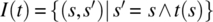
- Fault Tolerance. In order to be an adequate specification for fault tolerance, a specification has to meet the following criteria: first, lend itself to a simple, reliable oracle (the same criterion as for testing, for the same rationale); second, it has to lend itself to an efficient run-time execution (since it may have to be checked at run-time to detect errors); third, and most importantly, it has to refer to current states rather than current and past states. In practice, this third requirement means that the specification is represented by an inverse vector, that is, a relation R such that
 . Such relations refer to the current state but not to any previous state; they offer the advantage that they can be checked by looking exclusively at the current state and spare us from the burden of storing previous states at designated checkpoints and from checking complex binary relations; hence they represent a savings in terms of memory space and processing time.
To illustrate the kind of rationale that governs the mapping of sub-specification to methods, we consider the following examples:
- We consider the example of the sorting routine discussed in Chapter 6, where we showed that such a program is difficult to prove using static methods, and difficult to test, but that that it is easy to prove its correctness with respect to some part of the specification and very easy and efficient to test it against the other part of the specification.
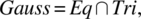
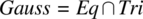
- We consider the specification of a program to perform a Gaussian elimination of a system of linear equations defined by a square matrix of size N and a column vector of size N. The specification that we consider for this program has the form:where Eq means that the original system of equations has the same set of solutions as the final system of equations and Tri means that the final system of equations is triangular. It is difficult to prove the correctness of the program with respect to specification Gauss (since this requires that we deal with several nested loops, we check the start and end values of several index variables, we worry about the logic for finding optimal pivots, etc.); it is very complex, inefficient, and unreliable to test the program using an oracle derived from specification Gauss (due to the difficulty and inefficiency of ensuring that two systems of equations have the same set of solutions); it gives us a great return on investment (in terms of required effort vs. achieved impact) to verify the correctness of a candidate program with respect to specification Eq (since that can be done by merely checking that the system of equations is never modified except by replacing an equation by a linear combination of the equation with others) and to test it using an oracle derived from specification Tri (since this can be done by a simple scan of the lower half of the current matrix, without reference to any previously saved data). Note that as an equivalence relation, Eq is reflexive and transitive (hence satisfies the properties we have identified as making a specification adequate for proving correctness).
Hence when we say that the first step in designing a test driver is to decide what specification we want to test the program against, we mean it. The foregoing discussions illustrate in what sense and to what extent the software engineer does have some latitude in making this decision.
12.2 SELECTING A PROCESS
The structure of the test driver depends on the following (inter-dependent) parameters:
- The Goal of the Test. If the goal of the test is to certify the product or to rule on acceptance, then it is driven by the mandated test data; if the goal of the test is to find and remove faults, then it is driven by the observation of failures.
- Whether the Test Data is Extracted from a Prepared Set or Generated by a Random Data Generator. If the test data is extracted from a prepared test data set, then it runs until the set is exhausted; if the test data is generated at random (according to some law of probability) by a test data generator, then some other criterion must be used to determine when the test terminates.
- Whether the Test Must Stop at Each Failure or Merely Record the Failure and Continue. Depending on the process of testing, we may have to stop the test whenever the program fails; this applies in particular if the test cycle includes a repair phase, which takes place off-line.
- Whether Test Outcomes Are Recorded for Postmortem Analysis. In some cases, such as certification testing or acceptance testing, the only relevant outcome of the test is whether the candidate program has passed the test successfully; in other cases, such as cases where the test results are used to identify and remove faults, each test execution (or perhaps each execution that leads to failure) must be documented for postmortem analysis.
As an example, a certification test based on a predefined test set may look like this:
bool certified (){bool c=true; stateType s, init_s;while !(testSet.empty()){testSet.remove(s); init_s=s;g; // program under test; manipulates s, preserves init_s;c = c && oracle(init_s, s);}return c;}
This function returns true if and only if the candidate program runs successfully on all the test data in testSet. If the same test data set is used for debugging purposes, then the test driver may look as follows:
void testReport(){stateType s, init_s;while !(testSet.empty()){testSet.remove(s); init_s=s;g; // program under test; manipulates s, preserves init_s;if (oracle(init_s, s)) {successfulTest(init_s,s);}else {unsuccessfulTest(init_s,s);};}}
If we have a test data generator that can produce data indefinitely, and we are interested in running the test until the next failure (hopefully, the program will fail eventually, if not we have an infinite loop), then the test driver may look as follows:
void testUntilFailure(){stateType s, init_s;repeat{generateTestData(s); init_s=s;g; // program under test; manipulates s, preserves init_s;}until !oracle(init_s,s);unsuccessfulTest(init_s, s);}
12.3 SELECTING A SPECIFICATION MODEL
For simple input/output programs, the test driver templates we have presented in the previous section can be used virtually verbatim; all we need to do is instantiate the functions that generate test data and execute the oracle. But for software products that have an internal state, such as abstract data types (ADT’s), two complications arise:
- First, the oracle is not a closed form Boolean function, since the specification is represented by axioms and rules rather than by a closed form logic formula.
- Second, test data does not take the form of values assigned to variables but rather takes the form of method calls.
In this section, we discuss the design of test drivers for software products that carry an internal state; we cover, in turn, the case where test data is generated randomly, then the case where test data is pre-generated according to some criterion (such as those discussed in Chapter 9).
12.3.1 Random Test Generation
We consider the specification of a state-based software product in the form of axioms and rules, and we consider a candidate implementation in the form of a class (an encapsulated module that maintains an internal state and allows access to a number of externally accessible methods). In order to verify the correctness of the proposed implementation with respect to the specification, we resolve to proceed as follows:
- Verify the Implementation Against the Axioms. Each axiom of the specification can be mapped onto a Hoare formula, whose precondition is True and whose postcondition is a statement about the behavior specified by the axiom. We consider the following axiom in the specification of the stack ADT:
- stack(init.push(a).top)=a,
and we let g be a candidate implementation that has a method of the same name as each input symbol of the specification. Then to verify the correctness of the implementation we generate the following formula:
- v: {true}
g.init(); g.push(a); y=g.top();{y = a}
where y is a variable of type itemType and
ais a constant of the same type. Such formulas typically deal with trivial cases (by definition) and hence involve none of the issues that usually make correctness proofs complicated; in particular, they typically give rise to simple intermediate assertions and do not involve complex invariant assertion generation. - Test the Implementation Against the Rules. Rules are typically used to build an inductive argument linking the behavior of the specified product on simple input histories to its behavior on more complex input histories. The vast majority of rules fall into two broad classes: a class that provides that two input histories are equivalent and a class that provides an equation between the values of a VX operation at the end of a complex input history as a function of the value of the VX operation at the end of a simpler input history. Representative examples of these categories of rules for the stack specification include the following:
- stack(init.h.push(a).pop.h+) = stack(init.h.h+).
- stack(init.h.push(a).size) = 1+stack(init.h.size).
We resolve to test candidate implementations against specification rules by generating random sequences for h and h+ (the latter being necessarily nonempty) and checking these equalities for each random instance. For rules of the first category, which require that we check the equivalence of two states, we resolve to consider (as an approximation) that two states are equivalent if and only if they deliver identical values for all the XV operations.
In light of these decisions, we write the outermost structure of our test driver as follows:
#include <iostream>#include “stack.cpp”#include “rand.cpp”using namespace std;typedef int boolean;typedef int itemtype;const int testsize = 10000;const int hlength = 9;const int Xsize = 5;const itemtype paramrange=7; // drawing parameter to push()// random number generatorsint randnat(int rangemax); int gt0randnat(int rangemax);// rule testersvoid initrule(); void initpoprule(); void pushpoprule();void sizerule(); void emptyrulea(); void emptyruleb();void vopruletop(); void voprulesize(); void vopruleempty();// history generatorvoid historygenerator(int hl, int hop[hlength], itemtype hparam[hlength]);/* State Variables */stack s; // test objectint nbf; // number of failuresint main (){/* initialization */nbf=0; // counting the number of failuresSetSeed (825); // random number generatorfor (int i=0; i<testsize; i++){switch(i%9){case 0: initrule(); break;case 1: initpoprule(); break;case 2: pushpoprule(); break;case 3: sizerule(); break;case 4: emptyrulea(); break;case 5: emptyruleb(); break;case 6: vopruletop(); break;case 7: voprulesize(); break;case 8: vopruleempty(); break;}}cout << “failure rate: ” << nbf << “ out of ” << testsize << endl;}
This loop will cycle through the rules, testing them one by one successively. The factor testsize determines the overall size of the test data; because test data is generated automatically, this constant can be arbitrarily large, affording us an arbitrarily thorough test. The variable nbf represents the number of failing tests and is incremented by the routines that are invoked in the switch statement, whenever a test fails. For the sake of illustration, we consider the function pushpoprule(), which we detail below:
void pushpoprule(){// stack(init.h.push(a).pop.h+) = stack(init.h.h+)int hl, hop[hlength]; itemtype hparam[hlength]; // storing hint hplusl, hplusop[hlength]; itemtype hplusparam[hlength]; // storing h+int storesize; // size in LHSboolean storeempty; // empty in LHSitemtype storetop; // top in LHSboolean successfultest; // successful test// drawing h and h+ at random, storing them in hop, hplusophl = randnat(hlength);for (int k=0; k<hl-1; k++){hop[k]=gt0randnat(Xsize);if (hop[k]==1) {hparam[k]=randnat(paramrange);}}hplusl = gt0randnat(hlength);for (int k=0; k<hplusl-1; k++){hplusop[k]=gt0randnat(Xsize);if (hplusop[k]==1) {hplusparam[k]=randnat(paramrange);}}// left hand side of rules.sinit(); historygenerator(hl,hop,hparam);itemtype a=randnat(paramrange); s.push(a); s.pop();historygenerator(hplusl,hplusop,hplusparam);// store resulting statestoresize = s.size(); storeempty=s.empty();storetop=s.top();// right hand side of rules.sinit(); historygenerator(hl,hop,hparam);historygenerator(hplusl,hplusop,hplusparam);// compare current state with stored statesuccessfultest =(storesize==s.size()) && (storeempty==s.empty()) && (storetop==s.top());if (! successfultest) {nbf++;}}
where function historygenerator (shown below) transforms an array of integers (which represent sequence h or h+) into a sequence of method calls, as shown below:
void historygenerator (int hl, int hop[hlength], itemtype hparam[hlength]){int dumsize; boolean dumempty; itemtype dumtop;for (int k=0; k<hl-1; k++){switch (hop[k]){case 1: {itemtype a=hparam[k]; s.push(a);} break;case 2: s.pop(); break;case 3: dumsize=s.size(); break;case 4: dumempty=s.empty(); break;case 5: dumtop=s.top(); break;}}}
and the random number generators are defined as follows:
int randnat(int rangemax){// returns a random value between 0 and rangemaxreturn (int) (rangemax+1)*NextRand();}int gt0randnat(int rangemax){// returns a random value between 1 and rangemaxreturn 1 + randnat(rangemax-1);}
We have included comments in the code to explain it. Basically, this function proceeds as follows: First, it generates histories h and h+; then it executes the sequence init.h.push(a).pop.h+, for some arbitrary item a; then it takes a snapshot of the current state by calling all the VX operations and storing the values they return. Then it reinitializes the stack and calls the sequence init.h.h+; finally it verifies that the current state of the stack (as defined by the values returned by the VX operations) is identical to the state of the stack at the sequence given in the left hand side (which was previously stored). If the values are identical, then we declare a successful test; if not, we increment nbf.
As an example of the second class of rules, those that end with a VX operation, we consider the size rule, for which we write the following code:
void sizerule(){// stack(init.h.push(a).size) = 1+stack(init.h.size)int hl, hop[hlength]; itemtype hparam[hlength]; // storing hint storesize; // size in LHSboolean successfultest; // successful test// drawing h and h+ at random,// storing them in hop, hplusophl = randnat(hlength);for (int k=0; k<hl-1; k++){hop[k]=gt0randnat(Xsize);if (hop[k]==1) {hparam[k]=randnat(paramrange);}}// left hand side of rules.sinit(); historygenerator(hl,hop,hparam);itemtype a=randnat(paramrange); s.push(a);// store resulting statestoresize = s.size(); // size value on the left hand side// right hand side of rules.sinit(); historygenerator(hl,hop,hparam);// compare current state with stored statesuccessfultest =(storesize==1+s.size());if (! successfultest) {nbf++;}}
Once we generate a function for each of the nine rules, we can run the test driver with an arbitrary value of variable testsize (to make the test arbitrarily thorough), an arbitrary value of variable hlength (to make h sequences arbitrarily large), and an arbitrary value of variable paramrange (to let the items stored on the stack take their values from a wide range).
Execution of the test driver on our stack with the following parameter values
-
testsize = 10000; -
hlength = 9; -
paramrange = 7;
yields the following outcome:
failure rate: 0 out of 10000
which means that all 10,000 executions of the stack were consistent with the rules of the stack specification. Of course, typically, when we are dealing with a large and complex module, a more likely outcome is to observe a number of failures. Notice that because test data generation and oracle design are both based on an analysis of the specification, we have written the test driver without looking at the candidate implementation; this means, in particular, that this test driver can be deployed on any implementation of the stack that purports to satisfy the specification we are using; we will uncover this implementation in Section 12.3.3.
12.3.2 Pre-Generated Test Data
In the previous section, we discussed how to develop a test driver using randomly generated test data. Because we had a way to generate data on demand, we focused the test driver on the rules of the specification; we let the rules determine what form the test data takes. In other words, for each rule, we generate test data that exercises the implementation of that rule. In this section, we take a different/complementary approach, which is driven by test data generation, in the following sense: we consider the test data that candidate implementations must be executed on, and for each test case, we design a test oracle by invoking all the rules that apply to the test case. This technique is best illustrated by an example, using the stack specification.
As we remember from Chapter 9, the criterion for visiting all the (virtual) states of the stack as well as making all the state transitions produced the following set of test data for stack implementations; so in order to meet this data selection criterion, we must run the candidate implementation on all these test sequences. As far as the test oracle is concerned, our discussions in Chapter 11 provide that for each sequence, we must invoke all the applicable rules and consider that candidate implementations are successful for a particular input sequence if and only if they satisfy all applicable rules.
| (X */E) | |||||||
| init | init.push (_) | init.push(_). push(_) | init.push(_). push(_). push(_) | ||||
| VX | top | init.top | init.push(a).top | init.push(_).push(a).top | init.push(_).push(_).push(a).top | ||
| size | init.size | init.push(a).size | init.push(_).push(a).size | init.push(_).push(_).push(a).size | |||
| empty | init.empty | init.push(a).empty | init.push(_).push(a).empty | init.push(_).push(_).push(a).empty | |||
| AX | VX | (X */E) | |||
| init | init.push (_) | init.push(_). push(_) | init.push(_). push(_). push(_) | ||
| init | top | init.init.top | init.push(a).init.top | init.push(_).push(a).init.top | init.push(_).push(_).push(a).init.top |
| size | init.init.size | init.push(a).init.size | init.push(_).push(a).init.size | init.push(_).push(_).push(a).init.size | |
| empty | init.init.empty | init.push(a).init.empty | init.push(_).push(a).init.empty | init.push(_).push(_).push(a).init.empty | |
| push | top | init.push(b).top | init.push(a).push(b).top | init.push(_).push(a).push(b).top | init.push(_).push(_).push(a).push(b).top |
| size | init.push(b).size | init.push(a).push(b).size | init.push(_).push(a).push(b).size | init.push(_).push(_).push(a).push(b).size | |
| empty | init.push(b).empty | init.push(a).push(b).empty | init.push(_).push(a).push(b).empty | init.push(_).push(_).push(a).push(b).empty | |
| pop | top | init.pop.top | init.push(a).pop.top | init.push(_).push(a).pop.top | init.push(_).push(_).push(a).pop.top |
| size | init.pop.size | init.push(a).pop.size | init.push(_).push(a).pop.size | init.push(_).push(_).push(a).pop.size | |
| empty | init.pop.empty | init.push(a).pop.empty | init.push(_).push(a).pop.empty | init.push(_).push(_).push(a).pop.empty | |
For the sake of illustration, we test a candidate implementation on a small sample of this test data set, specifically those test cases that are highlighted in the tables above. For each selected test case, we cite in the table below all the rules that apply to the case, as well as the input sequence that must be invoked in the process of applying the rule.
| Test case | Applicable Rule | Resulting Oracle |
| init.push(a).init.top | Init Rule | init.push(a).init.top = init.top |
| init.push(_).push(_).push(a).size | Size Rule | init.push(_).push(_).push(a).size = 1+init.push(_).push(_).size |
| init.push(_).push(a).push(b).empty | Empty Rule | init.push(_).push(a).empty ⇒ init.push(_).push(a).push(b).empty |
| init.push(_).push(_).push(a).pop.top | Push Pop Rule | init.push(_).push(_).push(a).pop.top = init.push(_).push(_).top |
To this effect, we develop the following program:
#include <iostream>#include <cassert>#include “stack.cpp”#include “rand.cpp”using namespace std;typedef int boolean;typedef int itemtype;const int Xsize = 5;const itemtype paramrange=8; // drawing parameter to push()// random number generatorsint randnat(int rangemax); int gt0randnat(int rangemax);/* State Variables */stack s; // test objectint nbtest, nbf; // number of tests, failuresitemtype a, b, c; // push() parametersbool storeempty;itemtype storetop;int storesize;int main (){/* initialization */nbf=0; nbtest=0; // counting the number of tests and failuresSetSeed (825); // random number generatora=randnat(paramrange); b=randnat(paramrange);c=randnat(paramrange);// first test case: init.push(a).init.top.// Init Rulenbtest++;s.sinit(); s.push(a); s.sinit(); storetop=s.top();s.sinit();if (!(s.top()==storetop)) {nbf++;}// second test case: init.push().push().push(a).size.// Size Rulenbtest++;s.sinit(); s.push(c); s.push(b); s.push(a); storesize = s.size();s.sinit(); s.push(c); s.push(b);if (!(storesize==1+s.size())) {nbf++;}// third test case: init.push().push(a).push(b).empty.// Empty Rulenbtest++;s.sinit(); s.push(c); s.push(a); s.push(b); storeempty=s.empty();s.sinit(); s.push(c); s.push(a);if (!(!(s.empty()) || storeempty)) {nbf++;}// fourth test case: init.push().push().push(a).pop.top// Push Pop Rulenbtest++;s.sinit(); s.push(c); s.push(b); s.push(a); s.pop(); storetop=s.top();s.sinit(); s.push(c); s.push(b);if (!(s.top()==storetop)) {nbf++;}cout << “failure rate: ” << nbf << “ out of ” << nbtest << endl;}
Execution of this program produces the following output:
failure rate: 0 out of 4.
Hence the candidate program passed these tests successfully. Combining the test data generated in Chapter 9 with the oracle design techniques of Chapter 11 produces a complex test driver; fortunately, it is not difficult to automate the generation of the test driver from the test data and the rules.
12.3.3 Faults and Fault Detection
The test drivers we have generated in Sections 12.3.1 and 12.3.2 are both based on the ADT specification and hence can be developed and deployed on a candidate ADT without having to look at the ADT. The executions we have reported in Sections 12.3.1 and 12.3.2 refer in fact to two distinct implementations:
- A traditional implementation based on an array and an index
- An implementation based on a single integer that stores the elements of the stack as successive digits in a numeric representation. The base of the numeric representation is determined by the number of symbols that we wish to store in the stack.
The motivation of having two implementations is to highlight that the test driver does not depend on candidate implementations; the purpose of the second implementation, as counterintuitive as it is, is to highlight the fact that our specifications are behavioral, that is, they specify exclusively the externally observable behavior of software systems, and make no assumption/prescription on how this behavior ought to be implemented. Also note that the behavioral specifications that we use do not specify individually the behavior of each method; rather they specify collectively the inter-relationships between these methods, leaving all the necessary latitude to the designer to decide on the representation and the manipulation of the state data. The header files of the two implementations are virtually identical, except for different variable declarations (an array and an index in the first case, a single integer, and a constant base for the second). The .cpp files are shown below:
********************************************************// Array based C++ implementation for the stack ADT.// file stack.cpp, refers to header file stack.h.//******************************************************#include “stack.h”stack :: stack (){};void stack :: sinit (){sindex =0;};bool stack :: empty () const{return (sindex==0);}void stack :: push (itemtype sitem){sindex++;sarray[sindex]=sitem;}void stack :: pop (){if (sindex>0){ // stack is not emptysindex--;}}itemtype stack :: top (){int error = -9999;if (sindex>0){return sarray[sindex];}else{return error;}}int stack :: size (){return sindex;}
As for the integer-based implementation, it is written as follows:
********************************************************// Scalar based C++ implementation for the stack ADT.// file stack.cpp, refers to header file stack.h.// base is declared as a constant in the header file, =8.//******************************************************#include “stack.h”#include <math.h>stack :: stack (){};void stack :: sinit (){n=1;};bool stack :: empty () const{return (n==1);}void stack :: push (itemtype sitem){n = n*base + sitem;}void stack :: pop (){if (n>1) { // stack is not emptyn = n / base;}}itemtype stack :: top (){int error = -9999;if (n>1){return n % base;}else{return error;}}int stack :: size (){return (int) (log(n)/log(base));}
In order to assess the effectiveness of the test drivers we have developed, we have resolved to introduce faults into the array-based implementation and the scalar-based implementation, and to observe how the test drivers react in terms of detecting (or not detecting) failure.
Considering the array-based implementation, we present below some modifications we have made to the code, and document how this affects the performance of the test drivers (the test driver that generates random test data, presented in Section 12.3.1, and the test driver that uses pre-generated test data, presented in Section 12.3.2).
| Locus | Modification | Random test data generation | Pre-generated test data |
pop();
|
sindex>0 → sindex>1
|
failure rate:
561 out of 10000
|
failure rate:
0 out of 4
|
push();
|
sarray[sindex]=sitem;
sindex++;
|
failure rate:
19 out of 10000
|
failure rate:
0 out of 4
|
push();
|
sindex++;
sarray[sindex]=sitem;
sindex++;
|
failure rate:
1964 out of 10000
|
failure rate:
1 out of 4
|
For the scalar-based implementation, we find the following results:
| Locus | Modification | Random test data generation | Pre-generated test data |
pop();
|
n>1 → n>=1
|
failure rate:
281 out of 10000
|
failure rate:
0 out of 4
|
sinit();
|
n=1 → n=0
|
failure rate:
822 out of 10000
|
failure rate:
0 out of 4
|
push();
|
n=n*base+sitem →
n=n+base*sitem
|
failure rate:
1047 out of 10000
|
failure rate:
2 out of 4
|
12.4 TESTING BY SYMBOLIC EXECUTION
When we deploy a test driver on some test data and the oracle is satisfied, the only evidence of correct behavior that we have collected pertains to the precise test data on which the candidate program was tested; whether the test driver relies on randomly generated test data, or on targeted, pre-generated test data, the space covered by test data is typically a very small fraction of the domain of the specification. To overcome this limitation, it is possible to simulate the execution of a program without committing to a particular value of the input; to this effect, we represent the input values by symbolic names, rather than actual concrete values and analyze the effect of executing the program on these values, so as to compare them with the requirements imposed by the specification. For all intents and purposes, this is essentially a static verification method, but it is considered as part of the toolbox of the software tester; we refer to this technique as symbolic testing because it consists in effect in testing a program by executing it symbolically (rather than actually) on symbolic data (rather than actual concrete data). Whereas actual program execution produces an actual output for a specific actual input value, symbolic execution produces a symbolic expression of the output as a function of a symbolic representation of the input; this amounts, in effect, to computing the function of the program. In Chapter 5, we had talked about program functions without discussing how these are derived; in this section, we briefly discuss how this can be done in a bottom-up stepwise process, which proceeds inductively on the program structure.
We can think of a program function as mapping inputs (from an input stream, say) onto outputs (stored in an output stream); but very often, it is more interesting and more convenient to think of a program function as mapping initial states to final states. To accommodate these two perspectives without too much complexity overhead, we generally focus on state transformation, but we may sometimes (especially when we discuss I/O operations) assume that we have a default input stream (is) and a default output stream (os) as part of the state space. We consider a simple C-like programming language, and we consider, in turn, its elementary statements and then its compound statements.
Elementary statements include assignment statements and input/output statements (which we denote respectively by read()and write()). We denote by S the space of the program (whose function we are computing), and by s and s′ arbitrary states of the program.
- Assignment Statement. Let x be a variable of some type T, let E be an expression on S that returns a value of type T, and let def(E) be the set of states on which expression E is defined (can be computed). Then

where
 (respectively
  ) designates all the variable names in s (respectively s′) other than x.
 - Read Statement. Let x be a variable of type T, and let is (the default input stream) be structured as a sequence of T-type values. Then,

where
 (respectively
  ) designates all the variable names in s (respectively s′) other than x and is.
 - Write Statement. Let x be a variable of type T, and let os be the default output stream of the program. Then,where

 (respectively
  ) designates all the variable names in s (respectively s′) other than os and
  designates concatenation.
Compound statements include the structured control constructs of imperative programming languages, most notably:
- The Sequence Statement, whose rule is defined as follows:
where · designates the relational product.
- The Conditional Statement, whose rule is defined as follows:

where
 .
. - The Alternative Statement, whose rule is defined as follows:

- The Iterative Statement, whose rule is defined as follows:

Because the formula of the while rule is difficult to apply in practice, we have a theorem that characterizes such functions.
In order to apply this theorem, we need to derive function W based on our understanding of what the loop does, then check that W verifies the conditions set forth above. We illustrate this theorem with two simple examples.
Let S be defined by variables x and y of type integer and let w be the following loop on S:
w: while (y!=0) {x=x+1; y=y-1;}.
We consider the following function W:
The first condition of the theorem is satisfied, since the domain of W is the set of states for which y is nonnegative, and that is exactly the set of states for which the loop terminates. As for the next two conditions, we check them briefly below:
= {substitution}
= {pre-restriction}
= {simplification}
= {substitution}
As for the third condition, we write
= {substitution, pre-restriction}
= {relational product}
= {simplification}
= {pre-restriction}
= {substitution}
As a second example, we let S be defined by natural variables n, f, k, and we consider the following loop on space S:
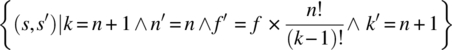
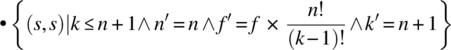
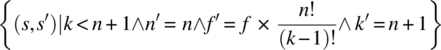
w: while(k!=n+1) {f=f*k; k=k+1;}.
We let W be the function on S efined by:
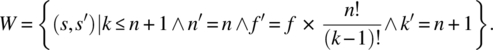
The domain of W is the set of states such that ![]() , which is precisely the set of states on which the loop terminates. We check in turn the two remaining conditions of the theorem, as follows:
, which is precisely the set of states on which the loop terminates. We check in turn the two remaining conditions of the theorem, as follows:
= {substitution}

= {pre-restriction}
= {simplification}
= {substitution}
As for the third condition, we write
= {substitution, pre-restriction}
= {relational product}

= {simplification}
= {pre-restriction}

= {substitution}
12.5 CHAPTER SUMMARY
In this chapter, we gather the artifacts we have collected in previous chapters to develop a test driver, which is responsible for running tests on a candidate software product and delivering a report from these tests. Specifically, we explore the following issues:
- In what sense and to what extent we have latitude in choosing the specification against which we can test a software product (whence the oracle that we derive for the test).
- How we can derive a test driver using a specific oracle (computed from a selected specification) and a specific test generation technique, for simple input/output programs and for software products that have an internal state.
- How we can overcome some of the limitations of software testing by means of symbolic execution, whereby we represent inputs by symbolic names (rather than concrete input values) and we represent outputs by symbolic expressions (rather than concrete output values).
12.6 EXERCISES
- 12.1 Consider the following C++ program:
void selectionSort () // given an array a of size N{indexType i, j, smallest;itemType t;for (i=N-1; i>0; i--){smallest=0;for (j=1; j<=i; j++){if (a[j]<a[smallest]) smallest=j;}t=a[smallest]; a[smallest]=a[i]; a[i]=t;}}- Prove the correctness of this program with respect to specification Sort.
- Derive an oracle for this program from specification Sort.
- Prove the correctness of this program with respect to specification Prm.
- Derive an oracle for this program from specification Ord.
- Conclude.
- 12.2 Same as Exercise 1, for a Gaussian elimination program, using the specification:
 .
. - 12.3 Consider the sort program of Exercise 1 and the specification Ord.
- Derive a test oracle from specification Ord.
-
Consider the following test set (giving values for
Nanda), build a set datatype that has the relevant methods (empty, insert, remove), and load the test data therein:Na[]1 [6] 2 [6, 9] 2 [9, 6] 8 [32, 28, 24, 20, 16, 12, 8, 4] 8 [32, 8, 24, 16, 4, 12, 20, 28] - Develop a test driver according to the pattern shown in Section 12.2 for certification testing.
- 12.4 Consider the sort program of Exercise 1 and the specification Ord.
- Derive a test oracle from specification Ord.
-
Consider the following test set (giving values for
Nanda), build a set datatype that has the relevant methods (empty, insert, remove), and load the test data therein:Na[]1 [6] 2 [6, 9] 2 [9, 6] 8 [32, 28, 24, 20, 16, 12, 8, 4] 8 [32, 8, 24, 16, 4, 12, 20, 28] - Develop a test driver according to the pattern shown in Section 12.2 for a test intended to record the outcome of each execution for subsequent analysis.
- 12.5 Consider the sort program of Exercise 1 and the specification Ord.
- Derive a test oracle from specification Ord.
- Alter the program in such a way as to make it incorrect.
-
Develop a random test data generator that produces random values for
Nanda. - Use the test data generator and the test oracle to develop a test driver that iterates until the first failure.
- How many executions did it take to cause the first failure?
- 12.6 In Section 12.3.1, we have shown the code for the push-pop rule. Taking inspiration from this code, write code for the init rule; run the resulting test driver on a candidate implementation of the stack.
- 12.7 In Section 12.3.1, we have shown the code for the push-pop rule. Taking inspiration from this code, write code for the init-pop rule; run the resulting test driver on a candidate implementation of the stack.
- 12.8 In Section 12.3.1, we have shown the code for the push-pop rule. Taking inspiration from this code, write code for the VX rules; run the resulting test driver on a candidate implementation of the stack.
- 12.9 In Section 12.3.1, we have shown the code for the size rule. Taking inspiration from this code, write code for the empty rule; run the resulting test driver on a candidate implementation of the stack.
- 12.10 In Section 12.3.1, we have shown the code for the size rule. Taking inspiration from this code, write code for the top rule; run the resulting test driver on a candidate implementation of the stack.
- 12.11 Consider the test data shown in the following table for the stack ADT. Select two test cases from each of the tables below and develop a test driver accordingly, following the pattern of Section 12.3.2 Deploy your test driver on the stack implementations given in Section 12.3.3.
(X */E) init init.push(_) init.push(_). push(_) init.push(_). push(_). push(_) VX top init.top init.push(a).top init.push(_).push(a).top init.push(_).push(_).push(a).top size init.size init.push(a).size init.push(_).push(a).size init.push(_).push(_).push(a).size empty init.empty init.push(a).empty init.push(_).push(a).empty init.push(_).push(_).push(a).empty AX VX (X */E) init init.push(_) init.push(_). push(_) init.push(_). push(_). push(_) init top init.init.top init.push(a).init.top init.push(_).push(a).init.top init.push(_).push(_).push(a).init.top size init.init.size init.push(a).init.size init.push(_).push(a).init.size init.push(_).push(_).push(a).init.size empty init.init.empty init.push(a).init.empty init.push(_).push(a).init.empty init.push(_).push(_).push(a).init.empty push top init.push(b).top init.push(a).push(b).top init.push(_).push(a).push(b).top init.push(_).push(_).push(a).push(b).top size init. push(b).size init.push(a).push(b).size init.push(_).push(a).push(b).size init.push(_).push(_).push(a).push(b).size empty init. push(b).empty init.push(a).push(b).empty init.push(_).push(a).push(b).empty init.push(_).push(_).push(a).push(b).empty pop top init.pop.top init.push(a).pop.top init.push(_).push(a).pop.top init.push(_).push(_).push(a).pop.top size init.pop.size init.push(a).pop.size init.push(_).push(a).pop.size init.push(_).push(_).push(a).pop.size empty init.pop.empty init.push(a).pop.empty init.push(_).push(a).pop.empty init.push(_).push(_).push(a).pop.empty - 12.12 Use the technique discussed in Section 12.3.1 to write a test driver for a queue implementation of the queue ADT. Write an array-based queue implementation and a scalar based queue implementation and deploy the test driver to test them.
- 12.13 Use the technique discussed in Section 12.3.2 to write a test driver for a queue implementation of the queue ADT. Write an array-based queue implementation and a scalar-based queue implementation and deploy the test driver to test them.
- 12.14 Let x and y be integer variables and let MaxInt and MinInt be (respectively) the largest (smallest) integer that can be represented in a given programming language. Compute (by symbolic execution) the function of the following statements.
-
x=x+1; -
y=y-1; -
x=x+1; x=x-1; -
x=x-1; x=x+1; -
x=x+1; y=y-1;
-
- 12.15 Let S be the space defined by variables x, y, z of type integer, and let w be the following while loop:
w: while (y!=0) {y=y-1; z=z+x;}And let W be the following function on S:

Prove that W is the function of
w. - 12.16 Let S be the space defined by integer variables x, y and z, and let w be the following while loop:
w: while (y!=0){if (y%2==) {y=y/2; x=2*x;} else {y=y-1; z=z+x;}}and let W be the following function on S:

Prove that W is the function of
w. - 12.17 Let S be the space defined by integer variables x, y and z, and let w be the following while loop:
w: while (y>0){if (y%2==) {y=y/2; x=2*x;} else {y=y-1; z=z+x;}}and let W be the following function on S:

Prove that W is the function of
w.
12.7 BIBLIOGRAPHIC NOTES
The theorem that captures the function of a program is due to H.D. Mills (1972). Because it requires a great deal of creativity (to derive a candidate function W), practitioners often replace it with an approximation of the loop function, whereby they do not compute the function of the loop for an arbitrary number of iterations (which is what this theorem does), but rather limit the number of iterations to a specific value and evaluate the function of the loop under these conditions; this produces an approximation of the program function, but still delivers much more information than a single execution of the program over a single input value.