
14
Metrics for Software Testing
The discipline of software metrics is concerned with defining quality attributes of software products and sizing them up with quantitative functions; such quantitative functions can then be used to assess the quality attributes of interest and thereby provide a basis for quantitative analysis and decision-making. Metrics have been used to capture such quality attributes as reliability, maintainability, modularity, verifiability, complexity, and so on. In this chapter, we focus our attention on software metrics that are relevant to testing and test-related attributes. We classify the proposed metrics into six categories that espouse the lifecycle of a system failure, namely:
- Fault proneness—the density of faults within the source code.
- Fault detectability—the ease of detecting faults in the source code.
- Error detectability—the ease of detecting errors in the state of a program in execution.
- Error maskability—the likelihood that an error that arises during the execution of a program gets masked before it causes a program failure.
- Failure avoidance—the ease of detecting and avoiding program failure with respect to its intended function.
- Failure tolerance—the likelihood that a program satisfies its specification despite failing to compute its intended function.
We review these metrics in turn, below. But first, we briefly introduce some elements of information theory, which we use in subsequent sections of this chapter. Given a random variable X on a finite set X (by abuse of notation we use the same name for the random variable and the set from which it takes its values), we let the entropy of X be the function denoted by H(X) and defined by:
where p(x) is the probability of occurrence of the event X=x and log is (by default) the base 2 logarithm. We take the convention that ![]() , and we find that H(X) is nonnegative for all probability distributions. H(X) is expressed in bits and represents the amount of uncertainty we have about the outcome of random variable X; for a set of given size n, this function takes its maximal value for the uniform distribution on X, where
, and we find that H(X) is nonnegative for all probability distributions. H(X) is expressed in bits and represents the amount of uncertainty we have about the outcome of random variable X; for a set of given size n, this function takes its maximal value for the uniform distribution on X, where ![]() for all x; the maximal value in question is then equal to log (n).
for all x; the maximal value in question is then equal to log (n).
Given a random variable X on set X and a random variable Y on set Y, we consider the joint random variable (X; Y) on the set ![]() with the probability distribution p2(x, y) on
with the probability distribution p2(x, y) on ![]() defined as the probability that variable X takes value x while variable Y takes value y. Then we define the joint entropy of X and Y as the entropy of the random variable (X; Y) on the set
defined as the probability that variable X takes value x while variable Y takes value y. Then we define the joint entropy of X and Y as the entropy of the random variable (X; Y) on the set ![]() with respect to the probability distribution p2(x, y). Using joint entropy, we let the conditional entropy of X with respect to Y be the function denoted by H(X|Y) and defined by:
with respect to the probability distribution p2(x, y). Using joint entropy, we let the conditional entropy of X with respect to Y be the function denoted by H(X|Y) and defined by:
The conditional entropy of X with respect to Y represents the uncertainty we have about the outcome of random variable X once we know what is the outcome of random variable Y.
If we let X be a random variable on set X and Y be a random variable on set Y, and if we let G be a function from X to Y then we have
where the probability distribution of Y is derived from that of X by the following formula:
Entropies and conditional entropies will be used to define some of the metrics that we discuss in the remainder of this chapter.
14.1 FAULT PRONENESS
What makes a software product prone to faults is its complexity; hence complexity metrics are adequate measures of fault proneness. Empirical studies routinely show a significant correlation between complexity metrics and fault density in software products. In this section, we present two widely known, routinely used metrics of structural complexity of control structures.
14.1.1 Cyclomatic Complexity
In its simplest expression, the cyclomatic complexity of a program reflects the complexity of its control structure and is computed by drawing the flowchart (say, F) of the program, then deriving the value of the expression as:
where
- e is the number of edges in F and
- n is the number of nodes in F.
We know from graph theory that if the flowchart is a planar graph (i.e., a graph that can be drawn on a planar surface without any two edges crossing each other) then v (F) represents the number of regions in F. Also, note that if the flowchart is merely a linear sequence of nodes, then its cyclomatic complexity is 1, regardless of the number of nodes; hence a single statement (corresponding to ![]() and
and ![]() ) has the same cyclomatic complexity as a sequence of 100 statements (
) has the same cyclomatic complexity as a sequence of 100 statements (![]() and
and ![]() ). This is consistent with our intuitive understanding of complexity as an orthogonal attribute to size: a sequence of 100 statements is longer than a single statement but is not more complex. As an illustration of this metric, we consider the following sample example:
). This is consistent with our intuitive understanding of complexity as an orthogonal attribute to size: a sequence of 100 statements is longer than a single statement but is not more complex. As an illustration of this metric, we consider the following sample example:
int product (int a, int b){int c; c=0;while (b!=0){if (b%2==0) {b=b/2; a=2*a;}else {b=b-1; c=c+a;}}return c;}
The flowchart of this program is given in Figure 14.1. From this flowchart, we compute the number of nodes and edges, and we find:
- e=7,
- n=6
whence
Figure 14.1 Counting nodes and edges.
Exercises 1 and 2 in Section 14.8 explore how this figure is affected after we make the program more complex by additional tests.
14.1.2 Volume
Whereas cyclomatic complexity measures the complexity of a program by considering the density of its control structure, the metric of program volume measures complexity by the amount of intellectual effort that it took to develop the program. We can argue that unlike the cyclomatic complexity, which measures structure independently of size, program volume captures size along with structural complexity. Specifically, program volume is computed as follows:
- If N is the number of lexemes (operators, operands, symbols, constants, etc.) in a program and
- n is the number of distinct lexemes (operators, operands, symbols, constants, etc.) in the program,
then the volume of the program is given by the following formula:
Interpretation: n is the size of the vocabulary in which the program is written; log2(n) measures the number of binary decisions one has to make to select one symbol in a vocabulary of size n; ![]() measures the total development effort of the program, viewed as the selection of N symbols in a vocabulary of size n, and quantified in terms of binary decisions. Alternatively, log2(n) can be interpreted as the entropy of the random variable that represents each symbol of the program and
measures the total development effort of the program, viewed as the selection of N symbols in a vocabulary of size n, and quantified in terms of binary decisions. Alternatively, log2(n) can be interpreted as the entropy of the random variable that represents each symbol of the program and ![]() is then the entropy of the whole program (quantity of information contained within its source text).
is then the entropy of the whole program (quantity of information contained within its source text).
If we consider again the product program given above, we find the following quantities:
- Number of lexemes, N: 66.
- Vocabulary: {int, product, (, a, ‘,’, b, ), {, c, ;, =, 0, while, !=, if, %, 2, ==, /, *, }, else, −, 1, +, return}. Hence n=26.
The volume of this program is:
Generating this program requires the equivalent of 310 binary (yes/no) decisions.
14.2 FAULT DETECTABILITY
Whereas complexity is a reliable indicator of fault proneness/fault density, the metrics we explore in this section reflect the ease of detecting the presence of faults (in a testing environment) or, conversely, the likelihood of fault sensitization (in an operating environment).
We consider a program g on space S and a specification R on S, and we let T be a test data set which is a subset of dom (R). Assuming that program g is faulty, we define the following metrics that reflect the level of effectiveness of T in exposing faults in g:
- The P-Measure, which is the probability that at least one failure is detected through the execution of the program on test data T.
- The E-Measure, which is the expected number of failures detected through the execution of the program on test data T.
- The F-Measure, which is the number of elements of test data T that we expect to execute on average before we experience the first failure of program g.
These metrics can be seen as indicators of the effectiveness of test set T in exposing program faults, but if we let T be a random test data set, then these metrics can be seen as characterizing the ease of exposing faults in program g.
These three metrics can be estimated in terms of the failure rate of the program (say, θ), which is the probability that the execution of the program on a random element s of the domain of R produces an image G (s) such that ![]() . Under the assumption of random test generation (where the same initial state may be generated more than once), we find the following expressions:
. Under the assumption of random test generation (where the same initial state may be generated more than once), we find the following expressions:
- The P-Measure. The probability that n tests generated at random do not cause the program to fail is
 . Hence the P-measure of the program is:
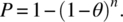
- The E-Measure. The expected number of failures experienced through the execution of the program on n randomly generated test data is:

- The F-Measure. Under the assumption of random test generation, the probability that the first test failure occurs at the ith test is
 . Statistical analysis shows that for this probability distribution, the mean (
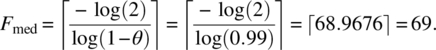
 ) and the median (Fmed) of the number of tests before the first failure are respectively:

where ![]() is the ceiling operator in the set of natural numbers.
is the ceiling operator in the set of natural numbers.
All these calculations depend on an estimation of θ, the probability of failure of the execution of the program on a randomly chosen initial state. This probability depends on the following two parameters:
- The set of initial states on which the candidate program g fails to satisfy specification R; as we have seen in Chapter 6, this set is defined (in relational form) as

- The probability distribution of initial states.
If the space of the program is finite and if the probability distribution is finite then the probability of failure can be written as:
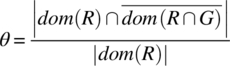
where ![]() represents set cardinality.
represents set cardinality.
As an illustrative example, we consider the space S defined by natural variables x, y, and z, and the following specification R on S.
We let g be the following program on space S:
g: {y = x+y; z = y%100;}
whose function is:
To estimate the probability of failure () of this program, we compute ![]() .
.
={substitution}
={simplification}
={taking the domain}
={logical simplification}
={logical simplification}
Taking the complement of this relation, we find:
={logic}
={since a mod 100 function returns values between 0 and 99}
Hence θ=0.01, since 99 is one value out of 100 that the mod function may take. With this value of probability failure, we can now compute the various measures of interest for a random test sample of size, say, 400:
- P-Measure.

- E-Measure.

- F-Measure.
- Mean:
- Median:
- Mean:
In other words, there is a 0.98205 probability that a random test of size 400 will expose at least one failure, the expected number of failures exposed by a random test of size 400 is four, the mean number of random tests before we observe the first failure is 100, and the median number of tests before we observe the first failure is 69.
Of course, in practice, these metrics are not computed analytically in the way we have just shown; rather they are estimated or derived empirically by extrapolating from field observations. Also regardless of how accurately we can (or cannot) estimate them, these metrics are useful in the sense that they enable us to reason about how easy it is to expose faults in a program and what test generation strategies enable us to optimize test removal effectiveness.
14.3 ERROR DETECTABILITY
What makes it possible to detect errors in a program? We argue that redundancy does; more specifically, what makes it possible to detect errors is the redundancy in the way program states are represented. When we declare variables in a program to represent data, we have in mind a relation between the data we want to manipulate and the representation of this data by means of the program variables. We refer to this relation as the representation relation; ideally, we may want a representation relation to have the following properties:
- Totality: each datum has at least one representation.
- Determinacy: each datum has at most one representation.
- Injectivity: different data have different representations.
- Surjectivity: all representations represent valid data.
It is very common for representation relations to fall short of these properties: in fact it is common to have none of them.
- When a representation relation is not total, we observe an incomplete representation: for example, not all integers can be represented in computer arithmetic.
- When a representation is not deterministic, we observe ambivalence: for example, in a sign-magnitude representation of integers, zero has two distinct representations, −0 and +0.
- When a representation is not injective, we observe a loss of precision: for example, real numbers in the neighborhood of a representable floating point value are all mapped to that value.
- When a representation is not surjective, we observe redundancy: for example, in a parity-bit representation scheme of bytes, not all 8-bit patterns represent legitimate bytes.
More generally, redundancy in the representation of data in a program stems from the non-surjectivity of the representation relation of program data, which maps a small data set to a vast state space of the program. If the representation relation were surjective, then all representations would be legitimate; hence if by mistake one representation were altered to produce another representation, we would have no way to detect the error; by contrast, if the representation relation were not surjective, and one representation were altered to produce another representation that is outside the range of the representation relation, then we would know for sure that we have an error. Hence the essence of state redundancy is the non-surjectivity of the representation relation. Whence the definition:
As an illustration, let us consider three program variables that we use to represent: the year of birth of a person, the age of the person, and the current year. The variable declarations of the program would look like:
int yob, age, thisyear;
If we assume that integer variables are coded in 32 bits, then the entropy of the program state is 3 × 32 bits = 96 bits. As for the entropy of the actual set of values that we want to represent, we assume that ages range between 0 and 150, years of birth range between 1990 and 2090 (101 different values), and current year ranges between 2014 and 2140 (127 different values). Because we have the equation yob+age = thisyear, the condition that age is between 0 and 150 is redundant and age can be inferred from the other two variables. Hence the entropy of the set of actual values is log(101) + log(127) = 27.62 bits. Hence the redundancy (excess bits) is 96 − 27.62 = 62.38 bits.
Now that we know how to compute the redundancy of a state, we use it to define the redundancy of a program: to this effect, we observe that while the set of program variables remains unchanged through the execution of the program, the range of values that program states may take shrinks, as the program establishes new relations between program variables; for example, a sorting routine starts with an array whose cells are in random order and rearrange them in increasing order. Given that the entropy of a random variable decreases as we apply functions to it, we can infer that the entropy of the final state of a program is smaller than the entropy of the initial state (prior to applying the function of the program) and the redundancy of the final state is greater than the redundancy of the initial state (assuming the set of program variables remains unchanged, that is, no variables have been declared or returned through the execution of the program). We can define the redundancy of a program by
- The state redundancy of its initial state, or
- The (larger) state redundancy of its final state, or
- The pair of values representing the initial and final state redundancies.
As an illustration, we consider the following program that reads two integers between 1 and 1024 and computes their greatest common divisor.
{int x, y; cin << x << y ;// initial stateWhile (x!=y) {if (x>y) {x=x-y;} else {y=y-x;}}// final state}
The set defined by the declared variables which are two integers; which we assume to be 32 bits wide; hence the entropy of the declared state is 2 × 32 bits = 64 bits. Because the variables range from 1 to 1024, the entropy of the set of values that these variables take is actually 2 × log(1024) = 20 bits. Hence the redundancy of the initial state is 44 bits. In the final state the two variables are identical and hence the entropy of the final state is merely log(1024), which is 10 bits. Hence the redundancy of the final state is 54 bits. The state redundancy of this program can be represented by the pair (44 bits, 54 bits).
14.4 ERROR MASKABILITY
Maskability is the ability of a program to mask an error that arises during its execution. In the testing phase, maskability may be seen as an obstacle to fault diagnosis, since (by definition) it masks errors and hence prevents the observer from exposing the impact of faults, while in the operating phase, maskability may be seen as a blessing, since it helps the program avoid failure. Either way, this metric is relevant from the standpoint of testing.
If we consider deterministic programs, tha is, programs that map initial states into uniquely determined final states, then each program defines an equivalence class on its domain that places in the same class all the initial states that map to the same final state. See Figure 14.2.
Figure 14.2 Measuring non-injectivity.
A program is all the more non-injective that the equivalence class of each final state is larger. To quantify this attribute, we let X be the random variable that represents the initial states of the program and we let Y be the random variable that represents the final states of the program. Then one way to quantify the size of a (typical) equivalence class is to compute the conditional entropy of X with respect to Y; in other words, we quantify the non-injectivity of a program by the uncertainty we have about the initial state of the program if we know its final state; the more initial states map to the same final state (the essence of non-injectivity), the larger this conditional entropy. Whence the definition:
Because Y is a function of X, this conditional entropy can simply be written as:
As illustrative examples, we consider the following:
- Let g be the following program on space S defined by a single integer variable i:
g = {i=i+1;}.Then , since
  , and
, and  , where w is the width of an integer variable. Ignoring the possibility of overflow, this program is injective; if variable i has an erroneous value prior to this statement, then it has an erroneous value after this statement.
 - Let g be the following program on space S defined by three integer variables i, j, and k:
g = {i=j+k;}Then , since
  , and
, and  , where w is the width of an integer variable. Indeed, this program has the potential to mask an error of size w: if variable i had a wrong value prior to this statement, then that error will be masked by this statement since the wrong value is overridden.
 - Let g be the following program on space S defined by three integer variables i, j, and k:
g = {i=0; j=1; k=2;}.Then , since
  , and
, and  , where w is the width of an integer variable. Indeed, this program has the potential to mask an error of size 3×w: if variables i, j, and k had wrong values prior to this statement, then that error will be masked by this statement since all the wrong values are overridden.
We submit the following interpretation:
The more non-injective a program, the more damage it can mask; in fact non-injectivity aims to measure in bits the amount of erroneous information that can be masked by the program.
14.5 FAILURE AVOIDANCE
Whereas state redundancy reflects excess information in representing a state, functional redundancy represents excess information in representing the result of a function. For example, if a function is duplicated (for the sake of error detection) or triplicated (for the sake of error recovery) then in principle we are getting one or (respectively) two extra copies, that is, two instances of excess information. But functional redundancy need not proceed in discrete quantities; as we define in this section, functional redundancy quantifies the (continuous) duplication of functional information. In the same way that state redundancy stems from the non-surjectivity of representation functions, functional redundancy stems from the non-surjectivity of program functions. Figure 14.3 illustrates graphically in what sense a duplicated function is more redundant than a single function, by virtue of being less-surjective: while the range of function F is isomorphic to the range of the duplicated function 〈F, F〉, the output space of 〈F, F〉 is much larger than the output space of F, making for a smaller ratio of range over output space, which is the essence of non-surjectivity.
Figure 14.3 Enlarging the output space, preserving the range.
Whereas we are accustomed to talking about a program space as a structure that holds input data and output data, in this definition we refer separately to the input space and the output space of the program. There is no contradiction between these two views: X may encompass some program variables along with input media (keyboard, sensors, input files, communication devices, etc.) and Y may encompass some program variables along with some media (screen, actuator, output file, communication devices, etc.).
As an illustration, we consider the following functions and show for each function: its input space (X), its output space (Y), its expression, its range (ρ), its functional redundancy (ϕ), and possibly some explanation of the result. We let B5 be the set of natural numbers that can be represented in a word of five bits.
| Name | Exp | X | Y | ρ | ϕ | Comments |
| F1 | X | B5 | B5 | B5 | 0 | All 5 bits are used |
| F2 | 2X | B5 | B5 | {0, 2, ..30} | 0.25 | Rightmost bit always 0 |
| F3 | X % 4 | B5 | B5 | {0,1,2,3} | 1.5 | 2 bits of information, 3 bits at 0 |
| F4 | X % 16 | B5 | B5 | {0,1,.. 15} | 0.25 | 4 bits of information, 1 bit at 0 |
| F5 | X/ 2 | B5 | B5 | {0,1,.. 15} | 0.25 | Leftmost bit always 0 |
| G1 | 〈F1, F1〉 | B5 | B5×B5 | B5×B5 | 1.0 | 1+2×φ(F1) |
| G2 | 〈F2, F2〉 | B5 | B5×B5 | {0, 2, ..30}2 | 1.5 | 1+2×φ(F2) |
| G3 | 〈F3, F3〉 | B5 | B5×B5 | {0, 1, 2, 3}2 | 4.0 | 1+2×φ(F3) |
| G4 | 〈F4, F4〉 | B5 | B5×B5 | {0, 1,.. 15}2 | 1.5 | 1+2×φ(F4) |
| G5 | 〈F5, F5〉 | B5 | B5×B5 | {0, 1,.. 15}2 | 1.5 | 1+2×φ(F5) |
14.6 FAILURE TOLERANCE
The quality attributes of software products such as reliability, safety, security, and availability depend not only on the products themselves but also on their specifications. Hence, if we want to define metrics that reflect software quality attributes, our metrics need to take into account specifications as well as software product per se. In this section, we consider a metric that captures relevant attributes of specifications.
Functional redundancy, which we have discussed in the previous section, reflects the ability of a software product to avoid failure and compute the intended behavior despite the presence and sensitization of faults and the emergence of errors. But if a specification is sufficiently non-deterministic, a program may fail to compute its exact intended function and still satisfy the specification. The question that we raise in this regard is: How do we measure the extent to which a program may deviate from its intended behavior without violating its specification. The measure of specification non-determinacy is an attempt to answer this question.
The conditional entropy of Y with respect to X represents the uncertainty we have about the value of Y if we know the value of X. The bigger the non-determinacy of R, the bigger this conditional entropy. As an illustrative example, we consider the following relation on space S defined by three variables i, j,and k.
The non-determinacy of this relation is ![]() . The reader may notice that (in this particular case) the inverse of relation R is a function; in other words, X is a function of Y, hence the join entropy H(X,Y) is the same as the entropy of Y. Hence the non-determinacy of this specification can be written as:
. The reader may notice that (in this particular case) the inverse of relation R is a function; in other words, X is a function of Y, hence the join entropy H(X,Y) is the same as the entropy of Y. Hence the non-determinacy of this specification can be written as:
In order to derive the entropies of X and Y, we must first compute the domain and range of relation R. We find:
Hence, under the assumption of uniform probability distribution, we find ![]() , since we have only two independent variables (i and j), and
, since we have only two independent variables (i and j), and ![]() , since we have three independent variables. We find:
, since we have three independent variables. We find:
which we interpret as follows: A program may lose as much as w bits of information (i.e., the width of an integer value) and still not violate specification R. Indeed, specification R mandates final values for i and j, but no final value for k, which means that a candidate program may lose track of k and still be correct; this is the meaning of non-determinacy.
14.7 AN ILLUSTRATIVE EXAMPLE
As further illustration, we consider the following sorting program and briefly compute its metrics as well as the non-determinacy of three possible sorting specifications that the program may be tested against.
int N=100;void sort (){int c, d, p, swap; c=0;while (c<N-1){p=c; d=c+1;while (d<N) {if (a[p]>a[d]) {p=d;} d++;}if (p!=c) {swap=a[c]; a[c]=a[p];a[p]=swap;} c++;}}
14.7.1 Cyclomatic Complexity
If we draw the flowchart of this program, we find that it has 14 edges and 11 nodes. Hence its cyclomatic complexity is 14 − 11 + 2 = 5.
14.7.2 Volume
If we analyze the source code of this program, we find that it has 108 lexemes taken from a vocabulary of 27 distinct lexemes. The volume of this program is:
14.7.3 State Redundancy
If we assume that integer variables are represented by 32 bits, then the entropy of the state of this program is 104 × 32 bits = 3328 bits. Now, if we assume that the cells of the array (as well as variable swap) range between 1 and 400 and that index variables (c, d, p) range between 0 and 100, then the entropy of the random variable that represents the initial data of the program is 101 × log(400) + 3 × log(100) = 893 bits. Hence the state redundancy of the initial state is 3328 − 893 bits = 2435 bits.
In order to compute the state redundancy of the final state of this program, we refer to a result to the effect that when an array of size N is sorted, its entropy drops by ![]() . Hence the entropy of the final sorted array is
. Hence the entropy of the final sorted array is ![]() . For N = 100, this expression evaluates to 200 bits. Because the final values of variables c and d are determined by the program, they are not counted in the entropy of the final state; we only count the entropy of the array and that of variables p and swap. We find that 200 + log(101) + log(400) = 213 bits. Hence the redundancy of the final state is 3328 − 213 bits = 3115 bits. Therefore, the state redundancy of this program can be represented by the interval: [2435 bits … 3115 bits]; the state redundancy of the program evolves from 2435 initially to 3115 in the final state. State redundancy measures the bandwidth of assertions that can be checked between variables of the state; in the final state it is almost 10 integers’ worth of assertions (i.e., nearly 10 assertions that equate 2 integer expressions to each other).
. For N = 100, this expression evaluates to 200 bits. Because the final values of variables c and d are determined by the program, they are not counted in the entropy of the final state; we only count the entropy of the array and that of variables p and swap. We find that 200 + log(101) + log(400) = 213 bits. Hence the redundancy of the final state is 3328 − 213 bits = 3115 bits. Therefore, the state redundancy of this program can be represented by the interval: [2435 bits … 3115 bits]; the state redundancy of the program evolves from 2435 initially to 3115 in the final state. State redundancy measures the bandwidth of assertions that can be checked between variables of the state; in the final state it is almost 10 integers’ worth of assertions (i.e., nearly 10 assertions that equate 2 integer expressions to each other).
14.7.4 Functional Redundancy
According to the definition of functional redundancy, the functional redundancy of the sort program is obtained by the following formula,
where Y is the output space of the program and ρ is the (random variable representing the) range of the program. For the output space, we let Y be the space of the S program, whose entropy we have found to be 3328 bits. For the range of the program, we have computed its entropy in the previous section and found it to be 213 bits. Hence the functional redundancy of this program is:
Much of this redundancy stems from the fact that we are using 32-bit words (100 of them) to represent integers between 1 and 400 only (when 9 bits would have been sufficient). Another factor that further reduces the entropy of the output (hence increases its redundancy) is that the output array is sorted; as a result, each cell of the array limits the range of possible values for the remainder of the array (e.g., if the first cell is 200, then the remainder of the array is restricted to the range [201...400] rather than [1...400]).
14.7.5 Non-injectivity
The non-injectivity of a program is the conditional entropy of its input (or initial state) given its output (or final state). Because this program sorts arrays, we know that each sorted array of size N stems from N ! distinct initial arrays (assuming, as we do, that all array cells are distinct). If we take the hypothesis of uniform probability distribution, and if we focus on the array (rather than auxiliary index variables), we find that this conditional entropy is log(N !). According to Stirling’s approximation, this quantity can be approximated by
for N = 100.
14.7.6 Non-determinacy
While all the previous metrics reflect properties of the program, non-determinacy reflects properties of the specification that the program is intended to satisfy and against which it is judged and tested. We consider three possible specifications for the sort program and compute the non-determinacy of each:
- Ord, which specifies that the output is ordered.
- Prm, which specifies that the final array is a permutation of the initial array.
-
 .
.
According to the definition of non-determinacy, we must compute the conditional entropy ![]() , where X is the random variable that takes its values over the domain of the specification and Y is the random variable that ranges over the image set of X by R (i.e., such that
, where X is the random variable that takes its values over the domain of the specification and Y is the random variable that ranges over the image set of X by R (i.e., such that ![]() ). We find the following:
). We find the following:
- Ord: This specification provides that the output array is sorted but bears no relation to the input array. In this case,
 . The entropy of a sorted array of size N whose values may take V values (in our case
  ) is given by the formula
  . For
. For  and
and  , we find
  . This is the extent to which a candidate program can deviate from the function of sorting and still not violate the specification Ord.
 - Prm: This specification provides that the final array is a permutation of the initial array but it does not stipulate that it must be ordered. For an array of size N (whose cells we assume to be distinct), there exist N! distinct arrays that satisfy this specification. Under the assumption of uniform probability, this entropy is
 , which we estimate by means of the Sterling approximation as
  . This is the extent to which a candidate program can deviate from the function of sorting and still not violate the specification Prm.
 - Sort: Because this specification is deterministic,
 . Any deviation of a candidate program from the mission of sorting the array will violate this specification.
14.7.7 SUMMARY
The following table summarizes the discussion of the sorting routine’s metrics.
| Metric | Value | Unit | Interpretation/meaning/relation to testing | |
| Cyclomatic complexity | 5 | Fault proneness | ||
| Volume | 513.53 | Fault proneness | ||
| State Redundancy | 2435 3115 |
Bits | Bandwidth of assertions that can check for errors, in initial state and final state | |
| Functional Redundancy | 14.62 | Factor by which state space is larger than the result of the computation | ||
| Non-injectivity | 564 | Bits | Bandwidth of data that the program may lose and still recover spontaneously | |
| Non Determinacy | Ord | 2536 | Bits | Amount of data a program can lose and still manage to satisfy the specification |
| Prm | 564 | |||
| Sort | 0 | |||
14.8 CHAPTER SUMMARY
In this chapter, we have presented syntactic and semantic metrics that have relevance from the standpoint of software testing and fault analysis:
- Fault proneness—the density of faults within the source code.
- Fault detectability—the ease of detecting faults in the source code.
- Error detectability—the ease of detecting errors in the state of a program in execution.
- Error maskability—the likelihood that an error that arises during the execution of a program gets masked before it causes a program failure.
- Failure avoidance—the ease of detecting and avoiding program failure with respect to its intended function.
- Failure tolerance—the extent to which a program may satisfy its specification despite failing to compute its intended function.
14.9 EXERCISES
- 14.1. Consider the
productroutine given in Section 14.1.1. Imagine that for the sake of speeding up the calculation of the product, we add a test for(b%4==0),and if the test is positive we divide b by 4 and multiply a by 4. Change the program accordingly and compute the new cyclomatic complexity. - 14.2. Consider the
productroutine given in Section 14.1.1. Imagine that for the sake of robustness (to avoid divergence) we check whether b is nonnegative before we engage in the loop. Change the program accordingly and compute the new cyclomatic complexity. - 14.3. Consider the
productroutine given in Section 14.1.1. Imagine that for the sake of speeding up the calculation of the product, we add a test for(b%4==0),and if the test is positive we divide b by 4 and multiply a by 4. Change the program accordingly and compute the volume of the new program. - 14.4. Consider the
productroutine given in Section 14.1.1. Imagine that for the sake of robustness (to avoid divergence) we check whether b is nonnegative before we engage in the loop. Change the program accordingly and compute the volume of the new program. - 14.5. Redo the calculations of the P-measure, E-measure, and F-measures on the program given in Section 14.2, with respect to the following specification:

- 14.6. Redo the calculations of the P-measure, E-measure, and F-measures on the program given in Section 14.2, with respect to the following specification:

- 14.7. Draw the flowchart of the sort program shown in Section 14.7, and compute its cyclomatic complexity.
- 14.8. Continuing the discussion of Section 14.7.6, compute the non-determinacy of the following specification:
-
- EqSum ∩ Sort.
- EqSum ∩ prm.
-
14.10 BIBLIOGRAPHIC NOTES
The definition of cyclomatic complexity is due to Thomas McCabe (1976). The volume metric is due to Maurice Halstead (1977). The semantic metrics presented in this chapter are due to Mili et al. (2014). Other semantic metrics may be found in Bansyia et al. (1999), Etzkorn and Gholston (2002), Gall et al. (2008), Morell and Murill (1993), Morell and Voas (1993), and Voas and Miller (1993). For more information on Software Metrics, consult Abran (2012), Ebert and Dumke (2007), and Fenton and Pfleeger (1997). For more information on entropy functions and information theory, consult Csiszar and Koerner (2011).