

66 4. TOPIC AK-4
18
1 + 3 cos
π
t
2
3
3 sin
π
t
2
+
3
3.5t 1
19
– 5t
2
– 4
3t
6t 1
20
2 – 3t – 6t
2
–
t–t
2
2
2t 0
21
6 sin
π
t
2
–
6
6 cos
π
t
2
+
6
4t 1
22
7t
2
– 3
5t
t ½
23
3 – 3t + t
–t
2
+
t
3
1.5t 1
24
– cos
π
t–
3
– sin
π
t
3
2t 1
25
– 6t – 2t
2
– 4
5t 1
26
8 cos
2
π
t+
6
– sin
2
π
t–
6
6t 1
27
–3 – 9 sin
π
t
2
6
– cos
π
t
2
+
6
3.5t 1
28
– 4t
2
+ 1 – 3t
4t 1
29
t
2
+
t–
3
3t
2
+ t + 3
5t 1
30
cos
π
t
2
–
3
– sin
π
t
2
+
3
1.5t 1
4.2 SAMPLE PROBLEM
From the given equations of motion (4.1) of particle M dene an equation of path, position of particle M on path at
t = t
1
(sec), velocity, normal, tangent, and full accelerations of the particle M, and radius of curvature at t = t
1
. Show
the dened parameters on the graph.
x =
4
(cm)
t + 1
y = –4t – 4 (cm) (4.1)
z = 2t + 2 (cm)
t
1
= 0.
4.3 SOLUTION
Equations of motion (4.1) are parametric equations of particle M trajectory. To obtain an equation of trajectory on a
usual coordinate form we will exclude time t from the rst and second equations of the system, as well as from the
second and third equations. en:
xy = –16, (4.2)
y = –2z. (4.3)
67
Equation (4.2) expresses in plane xOy an equal-sided hyperbola, where the coordinate axes are its asymptotes. In
space this equation describes hyperbolic cylinder with the surface tracer line parallel to the axis Oz.
Equation (4.3) expresses a straight line on the plane yOz, which crosses the origin of the coordinate system. In space
it is a plane which contains the axis Ox.
To nd the velocity of the particle we need to nd the x, y, and z components of velocity:
v
x
= x
̇
= –
4
cm
,
(t + 1)
2
s
v
y
= y
̇
= – 4
cm
,
s
v
z
= z
̇
= 2
cm
.
s
en the magnitude of the velocity:
v = √v
x
2
+ v
y
2
+ v
z
2
=
2
4 +
5(t + 1)
4
cm
.
(t + 1)
2
s
Similarly, we can nd the x, y, and z components of the acceleration
a
x
= x
̈
=
8
; a
y
= y
̈
= 0; a
z
= z
̈
= 0.
(t + 1)
3
A magnitude of the full acceleration of the particle M:
a = √a
x
2
+ av
y
2
+ a
z
2
=
8
cm
.
(t + 1)
3
s
2
e coordinates, velocity, acceleration, and their x, y, and z components at time instant t = 0 are shown in Table 4.2.
Table 4.2
Coordinates, cm Velocity, cm/s Accereration, cm/s
2
Radius of Curvature, cm
x y z v
x
v
y
v
z
v a
x
a
y
a
z
a a
τ
a
n
ρ
4 -4 2 -4 -4 2 6 8 0 0 8 5.33 5.96 6.04
Tangent acceleration we nd by dierentiating module of velocity (4.3):
a
τ
=
dv
dt
dv
=
2 v
x
v̇
x
+ 2 v
y
v̇
y
+ 2 v
z
v̇
z
=
v
x
a
x
+
v
y
a
y
+
v
z
a
z
=
–4 ∙ 8
= – 5.33
cm
.
dt
2
√v
x
2
+
v
y
2
+
v
z
2
v
6
s
2
A negative sign for
dv
shows the particle motion is decelerated, and, hence, a
τ
⃗
and v
⃗
are collinear but opposite
to each other.
dt
Normal acceleration of particle at given time instant:
a
n
= √a
2
– a
τ
2
= √8
2
– 5.33
2
= 5.96
cm
.
s
2
4.3 SOLUTION
68 4. TOPIC AK-4
e radius of curvature of the trajectory at point where the particle M is located at t = 0
ρ =
v
2
=
6
2
= 6.04 cm.
a
n
5.96
e calculated values of a
τ
, a
n
, and ρ are also shown in Table 4.2.
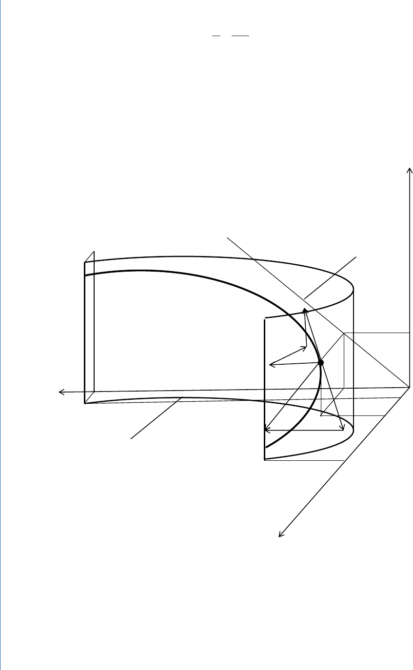
Using equation (4.2) we can draw a trajectory (Figure 4.1) and show a position of the particle M at the given time
instant. e vector v
⃗
is constructed by the components v
x
⃗
, v
⃗
y
, and v
z
⃗
. is vector v
⃗
must be tangent to the particle
trajectory. e vector a
⃗
we nd by components a
τ
⃗
and a
n
⃗
as well, which double checks the correctness of the calcu-
lations.
z
-y
x
0
1
4
16
-16
xy=-16
y+2z=0
-4
M
v
v
z
v
y
v
x
a
n
a=a
x
a
t
2
Figure 4.1.
..................Content has been hidden....................
You can't read the all page of ebook, please click here login for view all page.