3

Deforming Topology

In Chapter 2, we were introduced to the quad-based grids that make up models. One of the important functions topology serves is determining how a model is going to deform when using an armature, or doing a physics simulation. All of the rules that we learned are going to help us ensure that the model deforms the way that we want it to.

To get more comfortable with topology rules and how they relate to the deformations, we will be introduced to some standard joints and deforming geometries. We will work with bending joints, compressing and stretching meshes, and folding cloth using simulations.

The three rules discussed in this chapter are what I have discovered necessary to apply while working with 3D models that need to be bent, stretched, or twisted. In this chapter, you will understand both what these rules are and why they are important to apply.

In this chapter, we will be learning about the following subjects:

• Applying the bending and stretching deformation rule
• Applying the twisting deformation rule
• Applying the intersecting grids deformation rule
• Topology for cloth simulations

Applying the bending and stretching deformation rule

In Figure 3.1, you can see an elbow joint. This is one of the most common joints modeled on a mesh being deformed by an armature. Deformation refers to the bending or stretching of a mesh and is used to describe any shifting of the mesh after the mesh is finished.

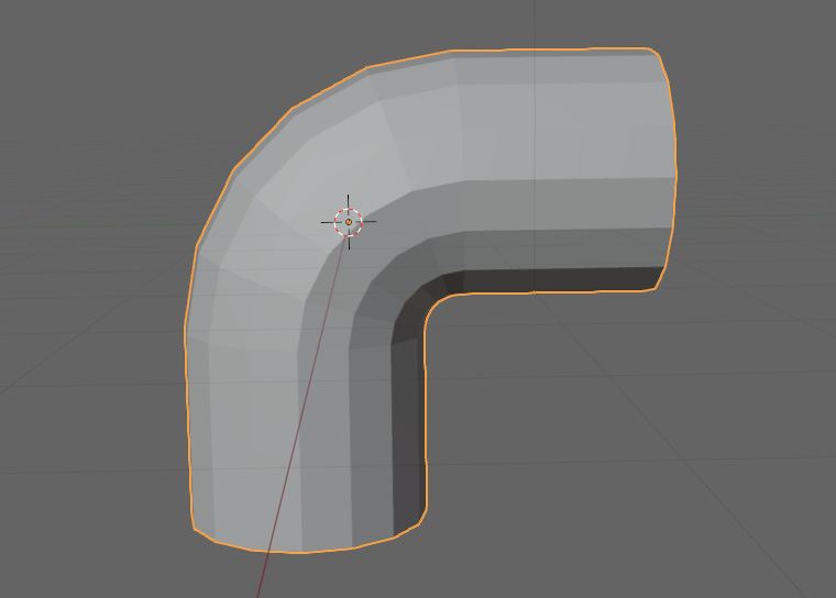
Figure 3.1 – An elbow joint

Our first deformation rule is that the edges of our grid need to be parallel to the axis of deformation. That is a bit of a mouthful, so we are going to break it down with a few examples. In Figure 3.2, we have a plane that has been bent around the y-axis.

Figure 3.2 – A plane bent around the y-axis

Go through the following steps to make this shape:

1. First, start by pressing Shift + A.
2. Add a plane from the mesh dropdown.
3. Then, go into Edit Mode.
4. Click on RMB, and select Subdivide.
5. In the bottom left of the Viewport, the Subdivide tab will appear – increase the number here until you are satisfied with the number of faces.
6. Select each of the edges and move them individually.
7. To move them along a specific axis, press G and then X, Y, or Z until it roughly matches Figure 3.2.

Now that we know how a plane is supposed to deform, we are going to look at how it is not supposed to deform. In Figure 3.3, you can see a lot of jagged corners have formed because we bent the plane the wrong way.

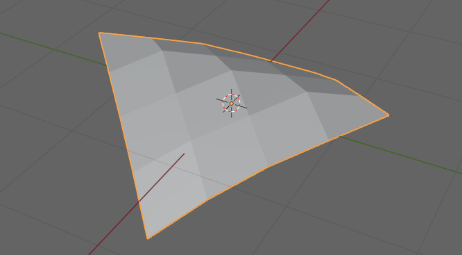
Figure 3.3 – Jagged corners resulting from bending the plane the wrong way

Because of the way the quads are positioned, we do not have a lot of control over which way the triangles are deforming. When we compare that to our mesh with the proper deformation in Figure 3.4, it is easy to tell the difference between the two.

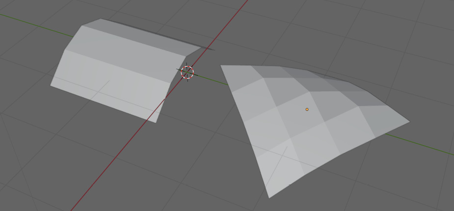
Figure 3.4 – Comparison between proper deformation (left) and improper deformation (right)

Next, we are going to look at a more commonly deformed shape, a cylinder. Remember, a cylinder has the same topology as a plane, just wrapped back into itself, so just like our plane, we need to bend it along the edges or make sure that our edges match up with our axis of deformation. If we were to bend it along the x-axis, it would look something like Figure 3.5. Notice how all of the loops of vertices wrapping around the mesh are in line with the x-axis. This holds true with any deformation axis you choose. It could be the x, y, or z-axis – or a random direction. Either way, the edges across the model need to be parallel to that axis of deformation.

Figure 3.5 – A properly deformed cylinder

Figure 3.6 shows a deformed cylinder that does not follow this rule.

Figure 3.6 – An improperly deformed cylinder

To get a better look at what is going on, we should reset this cylinder back to its original form. You can see this in Figure 3.7.

Figure 3.7 – A spiraling topology that can lead to improper deformation

This shape should feel familiar because we saw it in Figure 2.18 in Chapter 2, The Fundamentals of Topology. It was an example of a topology that breaks one of our topology rules: loops must not spiral down a mesh.

Figure 3.7 is an example of spiraling topology, and when trying to deform a joint, it can cause serious issues as shown before. Any time you have spiraling like this, you just have to isolate where it began and figure out how to connect it back into itself properly. In this case, you would have to shift the faces as illustrated in Figure 3.8.

Figure 3.8 – Shifting the face of the spiraling topology to correct the mismatch

These spirals are usually caused by a mismatch, so finding that mismatch usually fixes the issue. Looking back at our regular cylinder deform, if you focus on the bend like in Figure 3.9, you can see it still looks a little rough.

Figure 3.9 – Zooming in on the deformed pipe’s bend

The faces on the back look stretched, and the faces in the middle are squished.

You can try to fix this by adding more loops before deforming the cylinder, but it then causes the loops in the crease of the joint to become even denser. You can see it deformed again in Figure 3.10.

Figure 3.10 – The bend in the deformed pipe with more loops added

Likewise, if we remove too many from the inside, the back will stretch too much. What we want to do ideally is have more geometry on the back, and less geometry on the inside. Before we try to do this on an elbow joint, we should take a closer at stretching and compressing topology.

Our closer look at stretching and compressing, again, starts with a grid. If we look at Figure 3.11, we can see how a mesh is supposed to stretch and compress. You can see the left side stretches out, in the middle, it becomes a square again, and on the right, it is squished together.

Figure 3.11 – A stretched and compressed grid with the proper deformation

An example of a deformation we do not want can be seen in Figure 3.12.

Figure 3.12 – A stretched and compressed grid with improper deformation

You can see right away the preceding grid looks messy, and instead of compressing or stretching into rectangles, these rectangles stretch out across the corners and create diamond shapes. While it may not look bad while the plane is flat, if we start to bend it along the x or y-axis, it looks very rough. Figure 3.13 shows the two side by side.

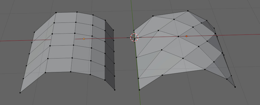
Figure 3.13 – Comparison of a properly deformed bent plane (left) and an improperly deformed bent plane (right)

And this is just a plane. The deformations get even worse when we move to more complex shapes. If we make a loop out of our plane, we can make something similar to an eyelid or mouth. This is a common shape in topology to manage something that needs to be able to stretch or compress radially. You can see the loops in Figure 3.14. It also shows the directions in which the topology should be able to stretch.

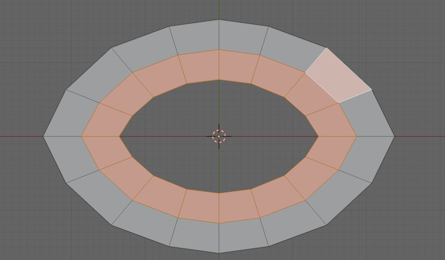
Figure 3.14 – A properly deformed plane looped to create a mouth or eyelid

If we deform our loop like an eyelid as in Figure 3.15, you can see that the faces that make up the topology retain more or less the same proportions, and the edges stay in line with the deformation.

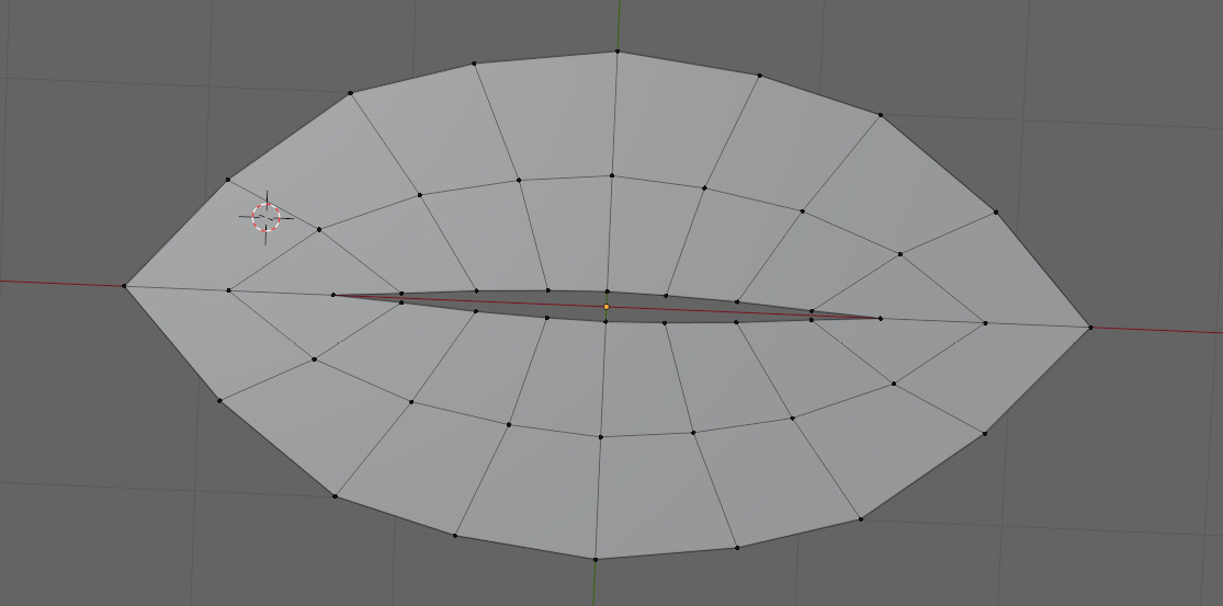
Figure 3.15 – A properly deformed plane looped to create an eyelid or mouth

As soon as you introduce lines that are not perpendicular to the stretching geometry, you get issues.

Identifying poor topology on a cylinder

Now that we know how poor topology might react to stretching on a plane, we can look at how it will affect a cylinder. You can see such a cylinder in Figure 3.16.

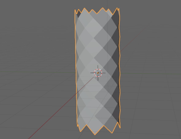
Figure 3.16 – A cylinder with poor topology

Immediately, it is easy to tell that something is off. The profile of the cylinder even looks weird. If we try to bend this model, it will result in a truly terrible deformation, as evident in this dreadful elbow joint in Figure 3.17.

Figure 3.17 – A bent cylinder with poor topology

In the preceding figure, the back is stretching much more than the previous elbow joint did, and the crease of the elbow is just as bad – just scrunched instead.

Fixing the topology on an elbow joint

Alright – we should take a closer look at that elbow joint we made earlier using a normal cylinder. We can see how it deformed again by looking back at Figure 3.5.

Figure 3.18 – A closer look at the elbow joint of a normal cylinder

We should try to see exactly where the mesh is stretching and compressing so that we can adjust the parts that we need to. Looking at Figure 3.19, we can see the specific areas we are having trouble with. On the outside of the joint, the faces are stretched out, and on the inside, the faces are scrunched.

Figure 3.19 – A closer look at the faces on the bend

An important thing to notice is the faces in between them. While the outside and inside of the joint deform a lot, the middle parts only deform a little bit. This is an important thing to keep in mind because it means we do not have to worry as much about these areas.

Then, the question we need to ask now is how do we actually manipulate the topology? Again, it is time for us to look at our grid. You can see our friendly grid in Figure 3.20.

Figure 3.20 – A 4x4 grid

What we are going to focus on first is adding more geometry to the back of the joint. One of the easiest and most consistent ways to add more geometry and have it follow our topology rules is to perform an extrusion using the following steps:

1. First, select the inner faces.
2. Then, press E to extrude the mesh.
3. Then, press S to scale.
4. Move the mouse to the desired scale.
5. And finally, use LMB to apply the transform.

When you are done extruding and scaling, it should look something like Figure 3.21. You will notice that the faces on the inside of the extrusion are much smaller than the ones surrounding it.

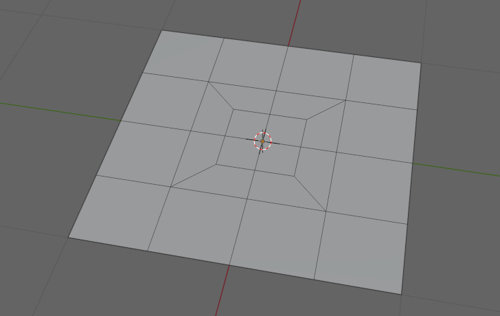
Figure 3.21 – Grid after extrusion and scaling

What allows the faces to shrink? If we take a closer look at it, we can see where the edges are forming this new geometry. Looking at Figure 3.22, we can see those poles on each of the corners of our extrusion.

Figure 3.22 – A view of the poles on the corners of the extruded grid

These are ultimately where the new geometry is coming from. If you think back to the last chapter, you might remember that these poles indicate a corner where two grids are intersecting. That is essentially what is happening here. These faces are highlighted in Figure 3.23 and are connecting the two grids that are not selected to add more geometry.

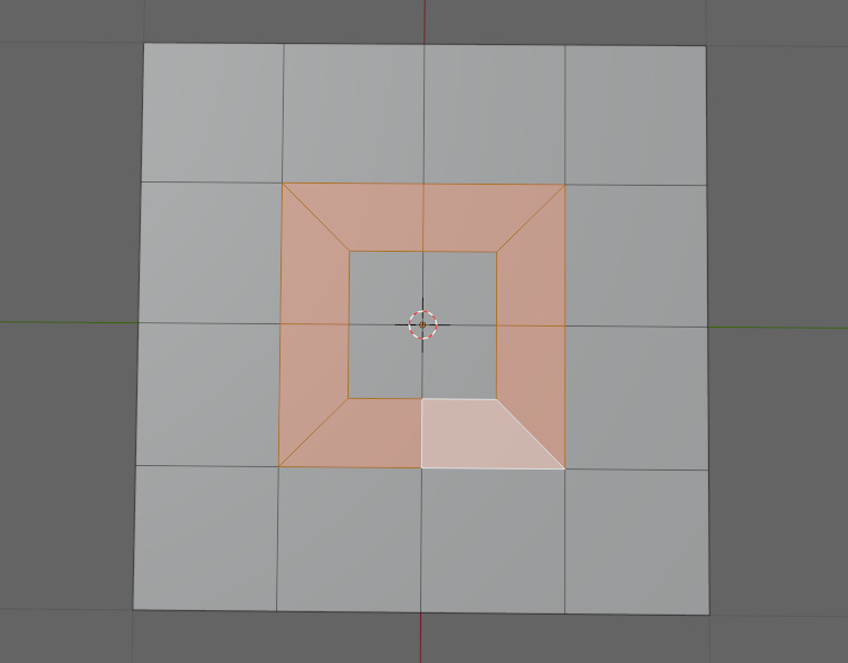
Figure 3.23 – The selected faces connecting the separate grids

This does cause a few problems right off the bat. Most notably, the faces connecting the two grids are warped quite a bit. We can help address this by moving the corners closer to the center point in the direction of the arrows in Figure 3.24.

Figure 3.24 – Moving corners closer to the center

This will help to distribute the distortion more evenly along the surface of the mesh. After you have repositioned the corners of the mesh, it should look something like Figure 3.25.

Figure 3.25 – Mesh with redistributed distortion

The second thing to note is that those sides joining the grids together are also still a lot longer than the smaller faces we just extruded. To start, we should try and compress one side of our new topology and see how it reacts. You can see it compressed in Figure 3.26.

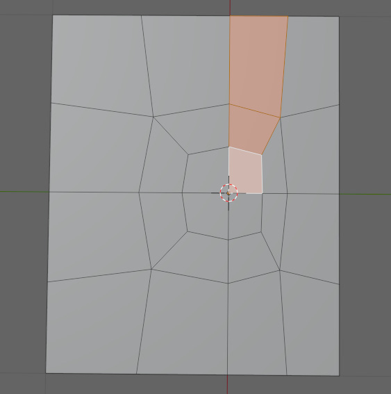
Figure 3.26 – Distorted topology with one side compressed

Overall, it looks pretty good. Almost all of the geometry is parallel or perpendicular to the direction in which we compressed it. The same thing can be said when stretching it as well. The only other major thing we need to worry about is how it bends, and this is where some issues start to pop up. If you remember, we are trying to stretch the denser part of the mesh, and compress the less dense areas.

You will notice that when we bend this mesh, some areas are denser than others, so it creates an uneven bend. This bend is visible in Figure 3.27.

Figure 3.27 – A bent mesh with an uneven bend

The issue here is caused by the long faces on the edges, and the shorter ones on the inside. The difference in shape is causing a difference in the deformation along the face. Remember, we are not actually applying this to a plane. We are applying it to a cylinder that is only deforming in one direction. To start, we are going to add our geometry to our cylinder. To do this, we are going to select the faces at the back of the joint and extrude them as we did on the plane. After extruding it and moving the vertices, it should look like Figure 3.28.

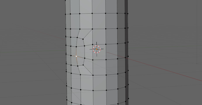
Figure 3.28 – Cylinder with extruded faces like the plane

The selection for the extrusion should be about halfway around the arm, with at least one row of faces below and above the loop of edges that will form our crease.

Now, we can give our new geometry a bend. In Figure 3.29, we can see how it should look.

Figure 3.29 – Bending our new geometry

Now that we can see it deformed, it looks pretty good. The quads are all mostly the same shape, and they are not being warped too drastically – that actually makes a lot of sense. If you recall our last example with the plane, the edges of the plane were much bigger than the middle ones, and the faces that transferred from the small ones to the big ones were small on one side and big on the other. If we compare a gradient of faces between a plane and a cylinder with the same topology, it is a bit easier to see. You can see a comparison in Figure 3.30.

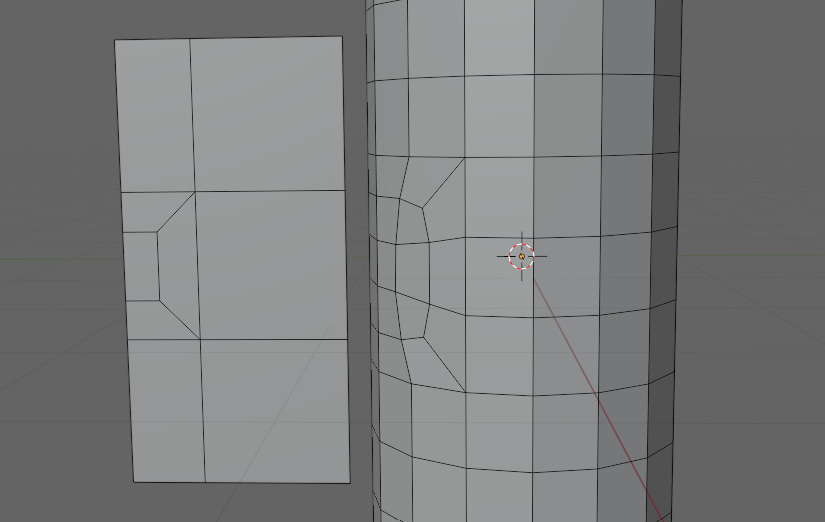
Figure 3.30 – Comparison of a plane (left) and a cylinder (right) with the same topology

The small faces are on the back so that they can be stretched out. The transitioning areas are on the sides, where they will transfer between the two sizes. The big faces are on the inside of the joint, where the faces are going to compress.

With that, we have managed to solve our deformation issues with the simple elbow joint. Now that we know how to deform our mesh with simple stretching and compressing, we can focus on some more joints.

Applying the twisting deformation rule

Twisting deformations are usually used on any shape that has one side rotate around an axis, while another part of that mesh either does not rotate or rotates the other way. You can see the result of this twisting happening to a cylinder in Figure 3.31.

Figure 3.31 – Twisting deformation on a cylinder

Notice how the edges connecting the top and bottom vertices are slanted. To achieve this, select the top face of the cylinder and press R and Z to rotate only the top face. Notice how we rotated them along an axis in line with the vertical edges, and perpendicular to the edges going around the cylinder. That is our second deformation rule, that the axis of twisting should be in line with the edge flow.

We can also use our good old grid to test this out too. In Figure 3.32, we can see our plane properly deformed along the edges in line with the red x-axis.

Figure 3.32 – A plane twisted around the x-axis

You will notice on both the cylinder and the plane that there are limitations to how far you can twist certain shapes. This is usually caused by too little geometry to work with. You can see the issue in Figure 3.33.

Figure 3.33 – A twisted cylinder with insufficient geometry

The preceding figure is reminiscent of the twisted end of a candy wrapper, which is why this problem is referred to as candy wrappering. It can be helped by adding more geometry to distribute the twisting across the faces a little bit more smoothly. If we look at Figure 3.34, we can see how this might look on a cylinder.

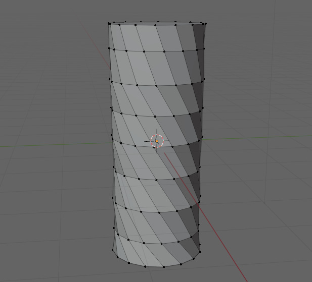
Figure 3.34 – A twisted cylinder with geometry added to smoothen faces

You might be able to notice the top and bottom loops of vertices are in the same place as in Figure 3.33. The only difference is in the middle, where we relaxed some of the loops by rotating the faces in the other direction.

Applying the twisting rule to shoulder deformations

Cylinders represent some of the easier shapes you can twist. It is much more difficult to have a joint twist within a hinged joint. These sorts of twists usually happen when a connection between two grids occurs. These sorts of connections are most commonly used to connect limbs to a body – for instance, the hip joint or the shoulder joint. Even the neck has a joint like this. Figure 3.35 shows us a simple shoulder topology.

Figure 3.35 – A shoulder topology

First off, we should look at our topology to see what it is doing. In this example, the front topology matches the back topology. At a first glance when looking at where the arm meets the shoulder, we can see a pole right where the armpit starts highlighted in Figure 3.36.

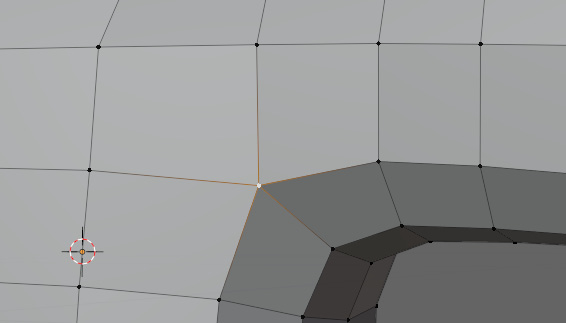
Figure 3.36 – A pole where the armpit starts

Because our mesh is mirrored front to back, and because we have one on the front, that means that there is another one on the back. If you remember, a pole indicates a corner of the intersection of two girds.

That means that we have two poles connecting the two grids. If we were to visualize this topology as straight grids, it would look something like Figure 3.37.

Figure 3.37 – Visualizing topology as straight grids

To improve the deformations around the pole where the arm meets, we are going to move the pole further away from the area of deformation. You can see the pole moved away from the joint in Figure 3.38.

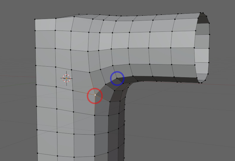
Figure 3.38 – Result of moving the pole further away from the joint

The blue circle marks where the pole used to be, and the red circle highlights the new position of the pole. Why exactly we do this may not be obvious at first, but with a few examples, it will hopefully make a bit more sense. In fact, this leads straight into our next rule.

Applying the intersecting grids deformation rule

Moving this pole is an example of the third deformation rule. Always have a buffer of at least one row of faces between a pole and the specific areas of deformation. You can see our new topology deforming in Figure 3.39.

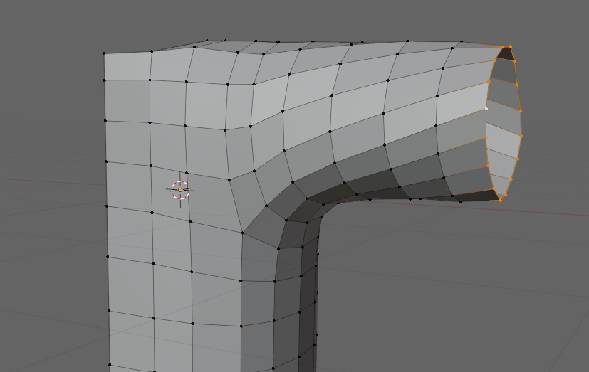
Figure 3.39 – Our new deformed topology with the third deformation rule applied

It is immediately noticeable that the transition is much smoother now that we have moved that pole further away from the area of deformation. This gave the geometry more room to do the deformation and reduced the amount of deformation the pole was experiencing as a result. Because a pole has edges pointing in more than just four directions, it is difficult to get it to deform cleanly. In Figure 3.40, you can see a plane with a regular four-edged vertex and another plane with a five-edged pole being deformed side by side.

Figure 3.40 – Comparison between a regular four-edged point (left) and a five-edged pole (right)

Because none of the edges are lined up with each other on the pole, it does not deform nicely like a normal quad.

You might ask yourself why you cannot just line up two of the edges so that they can deform cleanly. To a certain extent, you can do this, as Figure 3.41 shows us.

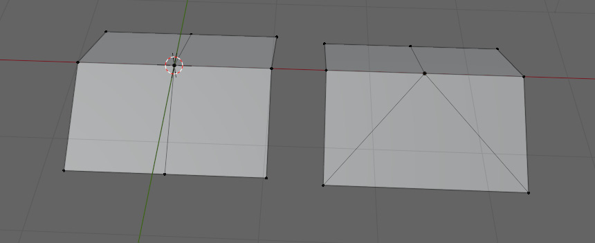
Figure 3.41 – Lining up edges to improve deformation

While aligning the edges in this fashion will work in this specific situation, as soon as we want to deform the mesh in any other way, this trick falls apart. This is shown in Figure 3.42.

Figure 3.42 – Deforming the mesh further makes lining up edges an inadequate solution

Instead of deforming around our lined-up edges, we deformed along a perpendicular axis. While we have one edge pointing in the correct direction on the top, the bottom edges form a V, causing it to behave erratically. That is why when deforming a pole, we always need to be mindful of the directions of deformation that are going to be applied to it. That way, we can avoid any unwanted topology artifacts caused by the mesh bending unpredictably.

Applying the intersecting grids rule to hip deformations

Now, we can try to apply this same way of thinking to the hip. You may remember making this shape in the final section of Chapter 2. Now that we have learned a few more things about how we approach deformations, we should take another look at that topology again to explain some of the reasons we made it the way we did. To start, we are going to look at another way we might approach the topology of that shape in Figure 3.43.

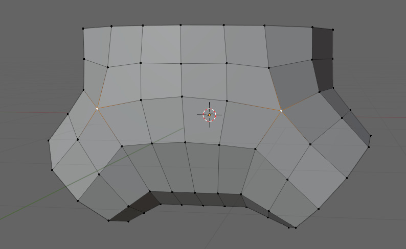
Figure 3.43 – The old example of the topology of this shape

This topology is identical to the topology we covered in the previous chapter, except for one difference. The pole in this example is positioned directly on the area of deformation. As we just learned from our previous rule, there needs to be a row of faces between a pole and the area of deformation. If we move our pole away from this area, you can see the solution to this in Figure 3.44.

Figure 3.44 – A new perspective of the hip topology with the pole positioned on the area of deformation

Now that we have applied the three rules of deformation to common shapes other than a plane, let us see how they relate to a simple cloth simulation.

Topology for cloth simulations

Just like normal deformations, cloth and soft body simulations follow the three deformation rules as well. While we will not get into the specific settings to apply to a soft body mesh, it is important to understand how the topology is going to react.

To start, subdivide a plane to make sure that our mesh has enough geometry to work with. Because the cloth simulation can be affected by the modifier stack, we should do as much of the subdividing as we can in the Modifiers tab. Be careful with the Subdivision modifier though – adding too many subdivisions can massively slow down your computer or outright crash Blender. We can see the Subdivision modifier in Figure 3.45.

Figure 3.45 – Subdividing the plane

To start out, do the following:

1. Add a Subdivision modifier set to Simple. This allows us to add more geometry without also smoothing the mesh.
2. To add a Cloth modifier, open the Modifier dropdown in the Modifiers tab.
3. Look under the Physics section.
4. Select the Cloth modifier. You can see this tab in Figure 3.46:

Figure 3.46 – Selecting the Cloth modifier

This will give us a simple cloth simulation when we run the simulation. The biggest determinant of the quality of a cloth deformation is the number of faces it has to work with. In Figure 3.47, you can see the same cloth settings run on meshes with different subdivision levels.

Figure 3.47 – Using the cloth setting on meshes with different subdivision levels

The left-hand model has two levels of subdivision, the center model has four, and the right-hand model has six. Of course, the more subdivisions you have, the longer the simulations will take – so what can we do to get the deformations we want without hiking up the simulation times?

Without touching the cloth settings, there are a few things we can do. The easiest option is to add another subdivision after the cloth modifier. In Figure 3.48, you can see the meshes with two subdivisions applied.

Figure 3.48 – Meshes with two subdivisions applied

Thus, one of the benefits of the cloth simulation being affected by the modifiers is that we can make changes to the simulation after the simulation is calculated. This means we can add as much detail as we want without having to worry too much about how it impacts the simulation speed. Ultimately, there are three things to worry about with simulations:

• You need to have really evenly sized quads to make sure that you get a consistent simulation. That means quads with edges that are even in size, and as close to square as possible.
• You need to make sure you have enough quads for the detail of the simulation you are trying to do.
• You need to apply the three deformation rules to it as well, especially for simulations with fewer quads.

This is all we will be discussing in relation to simulations, but it is important to touch on these to have a full understanding of topology, especially if you are going to be modeling clothes on characters and therefore using cloth simulations.

Summary

In this chapter, we learned how to approach a deformation problem. We also learned about the three deformation rules, including why the edges of our grid need to be parallel to the axis of deformation, why the axis of twisting should be in line with the edge flow, and why we must always ensure a buffer of at least one row of faces between a pole, and the specific areas of deformation. We also learned how to prepare a mesh for cloth simulation deformations.

Now that we know what rules to follow when deforming our topology, we can focus on our last major consideration before moving on to some real applications. In the next chapter, we will be looking at how UVs are affected by our topology, and how that can show us issues we may not have seen before.