
Chapter 5
Application to a distillation process
This chapter presents a second application study, which involves recorded data from an industrial distillation process, which is a debutanizer unit. Recorded data from this process were analyzed for process monitoring purposes using PCA and PLS (Kruger and Dimitriadis 2008; Kruger et al. 2008a; Meronk 2001; Wang et al. 2003).
Section 5.1 provides a description of this process. Section 5.2 then describes the data pre-processing and the identification of an MRPLS-based monitoring model. Finally, Section 5.3 analyzes a recorded data set that describes a severe drop in the fresh feed flow to the unit and shows how to detect and diagnose this event.
5.1 Process description
This process, schematically shown in Figure 5.1, is designed to purify Butane from a fresh feed comprising of a mixture of hydrocarbons, mainly Butane (C4), Pentane (C5) and impurities of Propane (C3). The separation is achieved by 33 trays in the distillation column. The feed to the unit is provided by an upstream depropanizer unit, which enters the column between trays 13 and 14. At trays 2 and 31 temperature sensors are installed to measure the top and bottom temperatures of the column.
Figure 5.1 Schematic diagram of debutanizer unit.
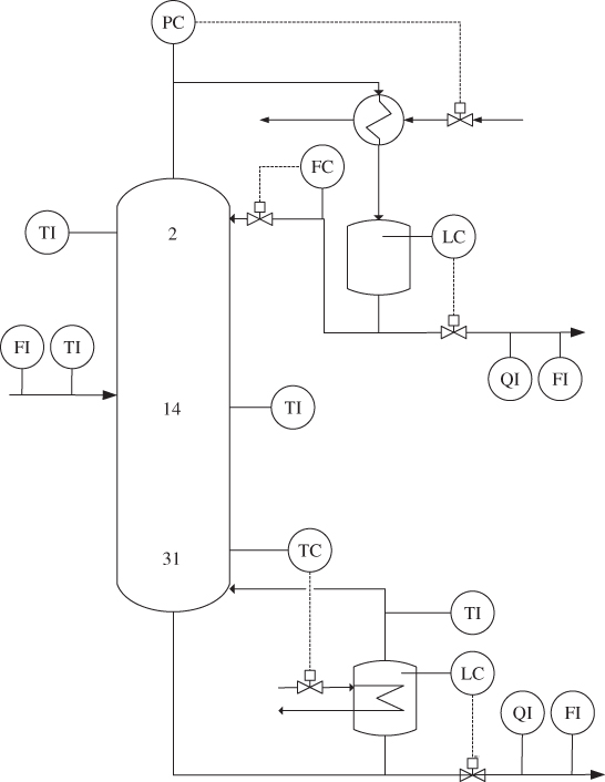
The lighter vaporized components C3 and C4 are liquefied as overhead product with large fan condensers. This overhead stream is captured in a reflux drum vessel and the remaining amount of C3 and C5 in the C4 product stream is measured through on-line analyzers. The product stream is divided into a product stream stored in butane tanks, and a reflux stream that returns to the column just above tray 1.
A second stream, taken from the bottom of the column, is divided between a feed entering the re-boiler and the bottom product. The temperature of the vaporized stream leaving the re-boiler and the C4 concentration in the bottom draw are measured. The bottom product is pumped to a mixing point, where it is blended into crude oil. Table 5.1 lists the recorded variables included in this study.
Table 5.1 Recorded process variables included in the MRPLS model
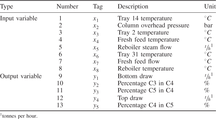
The reflux flow rate and the liquid level in the butane and reboiler tanks are omitted here, as they are either constant over the recording periods or controlled to a set-point and hence not affected by common cause variation. The remaining variable set includes the concentrations of C3 in C4, C5 in C4 (top draw) and C5 in C4 (bottom draw), flow rates of fresh feed, top and bottom draw, temperatures of the fresh feed, trays 2, 14 and 31, and the pressure at the top of the column.
This distillation unit operates in a closed-loop configuration. The composition control structure corresponds to the configuration discussed in Skogestad (2007):
- the top- and bottom draw flow rates control the holdup in the reflux drum and the reboiler vessel;
- the coolant flow into the condenser (not measured) controls the column pressure;
- the reflux flow rate, adjusted by a plant operator, controls the concentration of the distillate; and
- the temperature on tray 31 controls the concentration of the bottom product.
This configuration is known to achieve good performance for composition control but is also sensitive to upsets in the feed flow. Section 5.3 presents the detection and diagnosis of such an upset using the MSPC framework outlined in Chapters 1 to 3.
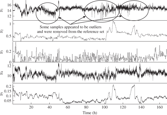
The variables related to product quality and the output of this process are the concentration measurements and the flow rates for top- and bottom draw. The remaining eight variables affect these output variable set and are therefore considered as the input variables. The next two sections describe the identification of a MRPLS model and the detection and diagnosis of a severe drop in the flow rate of the fresh feed. Figures 5.2 and 5.3 plot the reference data for the eight input and five output variables respectively, recorded at a sampling interval of 30 seconds over a period of around 165 hours.
Figure 5.2 Plots of reference data for input variables set.
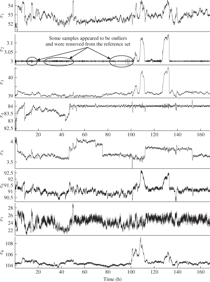
Figure 5.3 Plots of reference data for output variables set.
5.2 Identification of a monitoring model
The first step to establish a MRPLS model from the data shown in Figures 5.2 and 5.3 is to estimate the covariance and cross-covariance matrices ![]() ,
, ![]() and
and ![]() . Including a total of 20,157 samples (around 165 hours), (5.2) to (5.4) show these estimates. Prior to the estimation of these matrices, the mean value of each process variable was estimated and subtracted. In addition to that, the variance of each process variable was estimated and the process variables were scaled to unity variance. Equation (5.1) summarizes the pretreatment of the data
. Including a total of 20,157 samples (around 165 hours), (5.2) to (5.4) show these estimates. Prior to the estimation of these matrices, the mean value of each process variable was estimated and subtracted. In addition to that, the variance of each process variable was estimated and the process variables were scaled to unity variance. Equation (5.1) summarizes the pretreatment of the data
Equations 1.2, 1.3, 2.14 and 2.39 show how to estimate the variable mean and variance, as well as ![]() ,
, ![]() and
and ![]() .
.
Inspection of the entries in these matrices yields that:
- the only significant correlation within the output variable set is between the bottom and the top draw flow rates, and between the C4 in C5 and the C3 in C4 concentrations, producing a correlation coefficient of around 0.75 and 0.55, respectively;
- there is a very significant correlation of 0.95 between the column overhead pressure and the tray 2 temperature variables;
- there are significant correlation coefficients of 0.5 to 0.7 between all temperature variables; and
- further significant correlation within the input variable set are between the overhead pressure and the reboiler temperature and between the temperature reading of tray 14 and the fresh feed flow, again with correlation coefficients of 0.5 to 0.7.
The input variable set, therefore, shows considerable correlation among the pressure, the temperature variables and the flow rate of the fresh feed. This is expected and follows from a steady state approximation of the first law of thermodynamics.
5.3 
Using the estimated variance and cross-covariance matrices, the next step is the identification of a MRPLS model. Given that there are a total of eight input and five output variables, MRPLS can obtain a maximum of five sets of latent variables, whilst PLS/PCA can extract three further latent component sets for the input variable set. According to the data structure in 2.51, the identification of a MRPLS model entails (i) the estimation of the source signals describing common cause variation of the input and output variable sets and (ii) the estimation of a second set of latent variables that describes the remaining variation of the input variable set.
Figure 5.4 shows the results of applying the leave-one-out cross validation stopping rule, discussed in Subsection (2.4.2). A minimum of the PRESS statistic is for n = 4 sets of latent variables, suggesting that there are four source signals describing common cause variation of the input and output variable sets.
Figure 5.4 Cross-validation results for determining n.

Table 5.2 shows the cumulative contribution of the LV sets to ![]() ,
, ![]() and
and ![]() . These contributions were computed using 2.102 to 2.104, which implies that values of 1 are for the original covariance and cross-covariance matrices and values close to zero represent almost deflated matrices.
. These contributions were computed using 2.102 to 2.104, which implies that values of 1 are for the original covariance and cross-covariance matrices and values close to zero represent almost deflated matrices.
Table 5.2 Performance of MRPLS model on reference data.
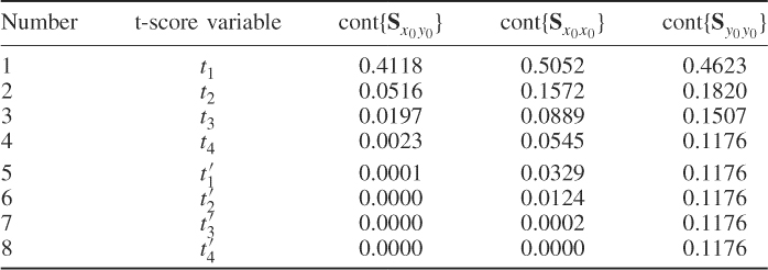
The first four rows in Table 5.2 describe LV contributions obtained from the MRPLS objective function in 2.68 and the deflation procedure in 2.74. The LV contribution representing rows five to eight relate to the PLS objective function in 2.76 and the deflation procedure in 10.18.
In terms of prediction accuracy, the rightmost column in Table 5.2 outlines that the first four LV sets rapidly reduce the squared sum of the elements in ![]() , which is evident by the reduction to a value of around 0.1 for the covariance matrix
, which is evident by the reduction to a value of around 0.1 for the covariance matrix ![]() . A similar trend can be noticed for the cumulative sum of the elements in
. A similar trend can be noticed for the cumulative sum of the elements in ![]() and
and ![]() . Different from the simulation example in Section 2.3.4, the common cause variation within input variable set is largely shared with the output variables. More precisely, the squared sum of the elements in
. Different from the simulation example in Section 2.3.4, the common cause variation within input variable set is largely shared with the output variables. More precisely, the squared sum of the elements in ![]() over those in
over those in ![]() is 0.055. For the cross-covariance matrix
is 0.055. For the cross-covariance matrix ![]() , a negligible ratio of 0.002 remains, as expected.
, a negligible ratio of 0.002 remains, as expected.
The application of PLS to the deflated covariance and cross-covariance matrices then allows deflating the covariance matrix ![]() by determining four further LV sets for the input variables. The variances of first four t-score variables are equal to 1, which follows from 2.65 and 2.66. The variances of the last four t-score variables
by determining four further LV sets for the input variables. The variances of first four t-score variables are equal to 1, which follows from 2.65 and 2.66. The variances of the last four t-score variables ![]() ,
, ![]() ,
, ![]() and
and ![]() are 0.6261, 0.2891, 0.4821 and 0.0598, respectively.
are 0.6261, 0.2891, 0.4821 and 0.0598, respectively.
Next, Table 5.3 lists the mean squared error (MSE) for predicting each of the output variable by including between 1 to 4 LV sets
5.5 
Apart from y3, that is, C5 in C4 concentration, the MRPLS model is capable of providing a sufficiently accurate prediction model. The prediction accuracy is compared by plotting the measured and predicted signals for each output variables below.
Table 5.3 Prediction accuracy of MRPLS model on referenced data.
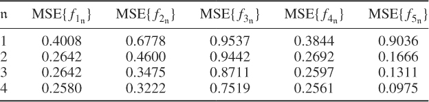
Obtaining a fifth set of latent variables using the MRPLS objective function, would have resulted in a further but insignificant reduction of the MSE values for each output variables: MSE![]() , MSE
, MSE![]() , MSE
, MSE![]() , MSE
, MSE![]() and MSE
and MSE![]() . This confirms the selection of four source signals that describe common cause variation shared by the input and output variable set.
. This confirms the selection of four source signals that describe common cause variation shared by the input and output variable set.
The issue of high correlation among the input variable set is further elaborated in Subsection 6.2.1, which outlines that the slight increase in prediction accuracy by increasing n from four to five may be at the expense of a considerable variance of the parameter estimation and, therefore, a poor predictive performance of the output variables for samples that are not included in the reference set.
Equations (5.6) and (5.7) show estimates of the r-weight and q-loading matrices, respectively.

To graphically interpret the relationship:
- between the computed t-score variables and the original input variables; and
- between the prediction of the output variables using the t-score variables
the elements of the r-weight and q-loading vectors can be plotted in individual loading plots, which Figure 5.5 shows. For the elements of the first three r-weight vectors (upper plot), most of the input variables contribute to a similar extent to the first three t-score variables, with the exception of the temperatures on trays 31 and 2.
Figure 5.5 Loading plots of first three r-weight vectors and q-loading vectors.
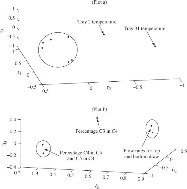
The main cluster suggests that the tray 14 temperature, the overhead pressure, the reboiler steam flow and the reboiler temperature have a very similar contribution to the computation of the t-score variables and hence, the prediction of the output variables. The first r-weight vector shows a distinctive contribution from the fresh feed flow and the upper plot in Figure 5.5 indicates a distinctive contribution from tray 2 and 31 temperatures to the computation of the t-score variables.
The t-score variables are obtained to predict the output variables as accurately as possible, which follows from 2.62 to 2.66. This implies a distinctive contribution from input variables tray 2, tray 31 and fresh feed temperature. This analysis makes sense, physically, as an alteration in the tray 31 temperature affects the concentration of the impurities in the top draw, changes in the tray 2 temperature impact the level of impurities (C4 in C5) of the bottom draw and alterations in the feed temperature can affect the impurity levels in the top and/or the bottom draw.
Now, inspecting the bottom plot in Figure 5.5 yields that the first three q-loading vectors produce distinctive patterns for:
- the flow rates of the top and the bottom draw;
- the C5 in C4 and C4 in C5 concentrations of the top and bottom draw; and
- an isolated pattern for the C3 in C4 concentration of the top draw.
Although prediction of the C5 in C4 concentration using the linear MRPLS regression model is less accurate compared to the remaining four output variables, it is interesting to note that the elements in the q-loading vectors suggest a similar contribution for each of the t-score variables in terms of predicting the C5 in C4 and the C4 in C5 concentration. The distinct pattern for the top and bottom draw flow rates is also not surprising, given that slight variations in the feed rate (x7) are mostly responsible for alterations in both output variables. This is analyzed in more detail below.
On the other hand, any variation in the C3 in C4 concentration is mostly related to the composition of the fresh feed. If the unmeasured concentration of C3 in this feed is highly correlated to the feed rate or temperature then those variables predict the C3 in C4 concentration. This outlines that the MSPC models are correlation-based representations of the data that do not directly relate to first-principle models representing causality, for example governed by conservation laws such as simple heat and material balance equations or more complex thermodynamic relationships. A detailed discussion of this may be found in Yoon and MacGregor (2000, 2001).
Assessing which input variable has a significant affect upon a specific output variable relies on analyzing the elements of the estimated regression matrix, which Table 5.4 presents. An inspection of these parameters yields that the fresh feed temperature has a major contribution to the C4 in C5 concentration but has hardly any effect on the remaining output variables. The negative sign of this parameter implies that the temperature increase results in a reduction of the C5 in C4 concentration.
Table 5.4 Coefficients of regression model for n = 4.
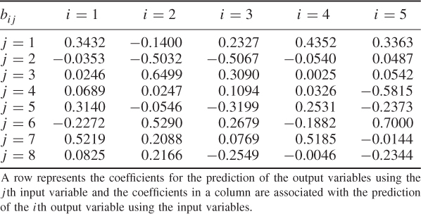
The flow rates of the top and bottom draw are mainly affected, in order of significance, by the fresh feed flow, the tray 14 temperature, the reboiler steam flow and the tray 31 temperature. Following from the preceding discussion, the tray 31 temperature has a distinctive effect on calculating the t-score variables, whilst the remaining three variables have a similar contribution. Knowing that the fresh feed flow and temperature are input variables that physically affect the temperatures, pressures and flow rates within the column, the analysis here yields that the most significant influence upon both output streams are the feed level and the tray 31 temperature.
For predicting the C3 in C4 concentration the column overhead pressure and the tray 2 and 31 temperatures are the most dominant contributors. However, C3 is more volatile than C4 and C5 and significant changes in the C3 in C4 concentration must originate from variations of the C3 concentration in the fresh feed. Moreover, Table 5.3 yields correlation between the concentrations of C3 in C4 and C4 in C5, and between the C3 in C4 concentration and the flow rates of both output streams.
Given this correlation structure and the fact that each of these three variables can be accurately predicted by the MRPLS regression model, it is not surprising that the C3 in C4 concentration can be accurately predicted too. This, again, highlights the fact that the MSPC model exploits the correlation between the input and output variables as well as the correlation within the input and output variable sets.
The remaining two variables to be discussed are the C5 in C4 and the C4 in C5 concentrations. With the exception of the fresh feed temperature and flow rate, each of the remaining variables contributed to the prediction of the C5 in C4 concentration. For the C4 in C5 concentration, the overhead pressure, the tray 2 temperature and the flow rate of the fresh feed did not show a significant contribution. The most dominant contribution for predicting the C5 in C4 and the C4 in C5 concentration is column overhead pressure and the tray 31 temperature, respectively.
A relationship between the overhead pressure and the C5 in C4 concentration is based on the estimated correlation structure. On the other hand, the positive parameter between the tray 31 temperature and the C4 in C5 concentration implies that an increase in this temperature coincides with an increase in the C4 in C5 temperature. The reason behind this observation, again, relates to the correlation structure that is encapsulated within the recorded variable set.
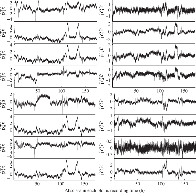
The analysis of the identified MRPLS model concludes with an inspection of the extracted source signals. Figure 5.6 shows the estimated sequences of the t-score variables that describe common cause variation of the input and output variable sets (Plot a) and sequences that describe the remaining variation within the input variable set only (Plot b). Following the MRPLS objective function, the t′-scores are not informative for predicting output variables.
Figure 5.6 Estimated t-score (a) and t′-score (b) variable sets.

Staying with the t-score variables Figure 5.7 shows the contribution of the estimated t-score variables (left plots) and the t′-score variables (right plots) to the input variables. As expected, with the exception of variables x2, x5 and x8, the variance contribution of the t-score variables is significantly larger than that of the t′-score variables to the input variable set.
Figure 5.7 Signal contributions of s (left plots) and s′ (right plots) to input variables.
Evaluating the remaining variance of the input variables after subtracting the contribution of the four t-score variables, which Figure 5.8 shows, confirms this. An approximate estimation of the residual variances is given by1
5.8 ![]()
and stored in ![]() . As before,
. As before, ![]() is the loading matrix and
is the loading matrix and ![]() is the t-score vector for the kth sample. As the variance of each of the original input variables is 1, the smaller the displayed value of a particular variable in Figure 5.8 the more variance of this input variable is used for predicting the output variables.
is the t-score vector for the kth sample. As the variance of each of the original input variables is 1, the smaller the displayed value of a particular variable in Figure 5.8 the more variance of this input variable is used for predicting the output variables.
Figure 5.8 Residual variance of input variables after deflation.
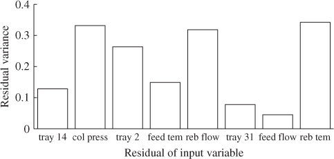
The smallest value is for the flow rate of the fresh feed, followed by those of the tray 31 temperature, the tray 14 temperature and the temperature of the fresh feed. The other variables are less significantly contributing to the prediction of output variables. After assessing how the t-score and the t′-score variables contribute to the individual input variables, Figure 5.9 shows the prediction of the output variables (left column) and the residual variables for the reference data set.
Figure 5.9 Model prediction (left column) and residuals (right column) of outputs.
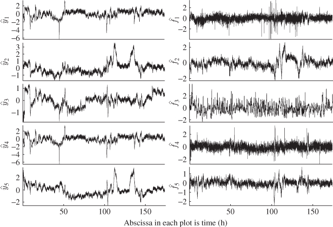
Apart from y3, describing the C5 in C4 concentration, the main common cause variation within the unit can be accurately described by the MRPLS model. Particularly the residuals of the output variables y1, y4 and y5 show little correlation to the recorded output variables.
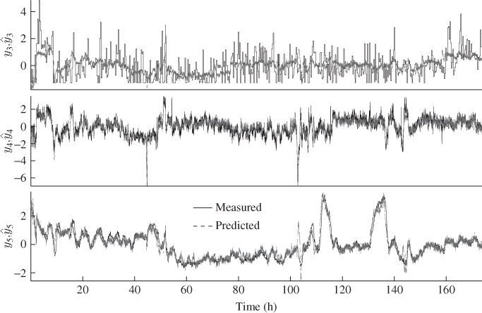
Figure 5.10 presents a direct comparison of the measured signals for variables y3 to y5 with their prediction using the MRPLS model. This comparison confirms the accurate prediction of y4 and y5 and highlights the prediction of the C5 in C4 concentration can describe long-term trends but not the short-term variation, which is the main factor for the high MSE value, listed in Table 5.3.
Figure 5.10 Measured and predicted signals of output variables y3 to y5.
5.3 Diagnosis of a fault condition
The process is known for severe and abrupt drops in feed flow which can significantly affect product quality, for example the C5 in C4 concentration in the top draw. The propagation of this disturbance results from an interaction of process control structure, controller tuning and operator support. The characteristics of this fault are described first, prior to an analysis of its detection and diagnosis. This fault is also analyzed in Kruger et al. (2007), Lieftucht et al. (2006a), Wang et al. (2003).
The feed flow, provided by a depropanizer unit, usually shows some variations that, according to Figure 5.2, range between 22 to 27![]() . This flow, however, can abruptly decrease by up to 30%. An example of such a severe drop is studied here, highlighting that the identified monitoring model can discriminate between the severity of feed variations and whether they potentially affect product quality.
. This flow, however, can abruptly decrease by up to 30%. An example of such a severe drop is studied here, highlighting that the identified monitoring model can discriminate between the severity of feed variations and whether they potentially affect product quality.
Figure 5.11 plots the recorded input variables for such an event, where a minor but prolonged drop in feed level is followed by a severe reduction that has significantly impacted product quality. The first minor drop in feed flow occurred around 23 hours into the data set with a reduction from 25 to 24![]() and lasted for about 3 hours. The second and severe reduction in feed level occurred around 26 hours into the data set and reduced the flow rate to around 17
and lasted for about 3 hours. The second and severe reduction in feed level occurred around 26 hours into the data set and reduced the flow rate to around 17![]() and lasted for about 2 hours.
and lasted for about 2 hours.
Figure 5.11 Data set describing impact of drop in feed level on input variable set.
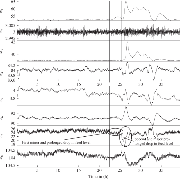
It should be noted that the level controllers in the bottom vessel, distillate drum and the column pressure can compensate the material balance within the column to fluctuations in the fresh feed level. The temperature controller, however, may be unable to adequately respond to these events by regulating the energy balance within the column if severe and prolonged reductions in feed arise. Figures 5.11 and 5.12 demonstrate this. The response of the column to the first prolonged drop is a slight increase the tray 14 temperature and a minor reduction in the reboiler steam flow.
Figure 5.12 Data set describing impact of drop in feed level on output variable set.
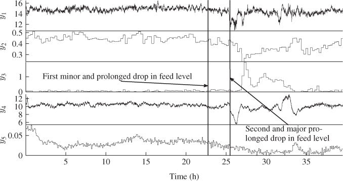
The second drop that followed had a significantly greater impact on the operation of the column. More precisely, each of the column temperatures, that is, v1, v3 and v6, increases sharply and almost instantly. Consequently, the C5 in C4 concentration (y3) rose above its desired level about 1.5h after the feed level dropped substantially around 26h into the data set. The effect of this drop in feed level was also felt in the operation of the reboiler, as the reboiler temperature v8 and the reboiler steam flow decreased. Another result of this event is a reduction of the flow rate of both output streams, y1 and y4. Figure 5.12 shows that the maximum drop of 7![]() is split into a reduction of 3 and 4
is split into a reduction of 3 and 4![]() in the flow rate of top and bottom draw, respectively.
in the flow rate of top and bottom draw, respectively.
Figure 5.2 shows that the feed level can vary slowly and moderately, which will introduce common cause variation within the unit. The issue here is to determine when a severe drop in feed arises that has a profound impact upon product quality. This is of crucial importance, as any increase in the C5 in C4 concentration arises with a significant delay of around 90 minutes. In other words, monitoring the output variable y3 or the input variable v7 alone is insufficient for the monitoring task at hand. This is because variations in the feed level naturally occur and may not necessarily lead to an undesired effect on product quality. The monitoring of this process thus requires a multivariate analysis in order to alert process personnel when a severe feed drop occurs. Meronk (2001) discussed a number of potential remedies to prevent the undesired increase of the C5 in C4 concentration.
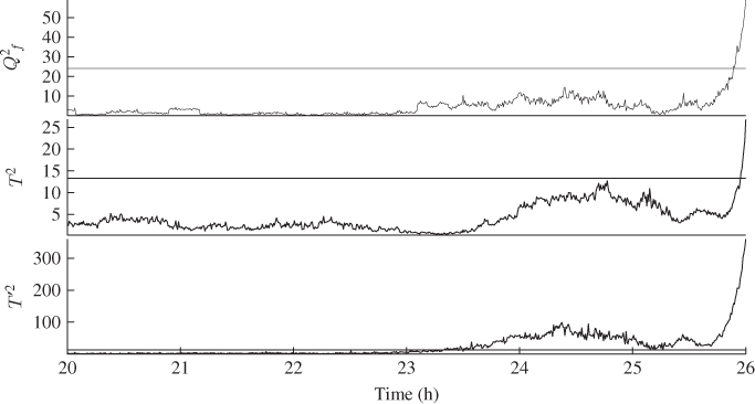
As outlined in Subsection 3.1.2, the multivariate analysis relies on scatter diagrams and non-negative quadratic statistics. Figure 5.13 shows the Hotelling's T2 and T′2, and the Qf statistics. As expected, the first 22 hours into the data set did not yield an out-of-statistical-control situation. The drop in fresh feed was first noticed by the Hotelling's T′2 statistic after about 23.5h, with the remaining two statistics showing no response up until 26h into the data set.
Figure 5.13 Monitoring statistics of data set covering drop in fresh feed level.
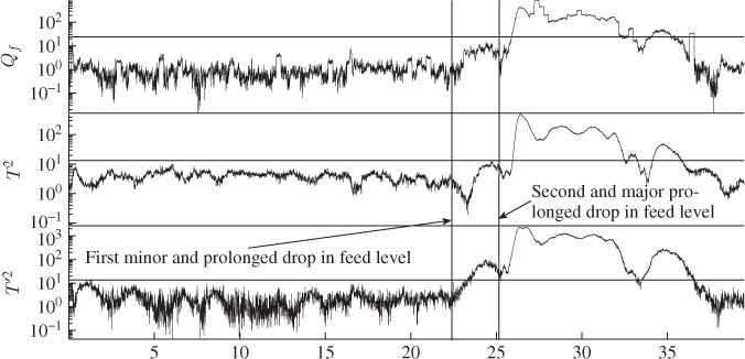
Figure 5.14 shows a zoom of each monitoring statistic in Figure 5.13 between 20 to 26h. The linear combinations of the input variables that are predictive for the output variables are not affected by the initial and minor drop in fresh feed. The Qf statistic also confirms this, since it represents the mismatch between the measured and predicted output variables and did not suggest an out-of-statistical-control situation during the first minor drop in feed. However, the correlation between the input variables that is not informative for predicting the output variables, that is, the remaining variation that contributes to the input variables only, is affected by the prolonged drop in the feed level. Particularly the increase in the tray 14 temperature and the decrease in the reboiler steam flow, according to Figure 5.11, is uncharacteristic for normal process behavior and resulted in the out-of-statistical-control situation.
Figure 5.14 Monitoring statistics for feed drop between 20 to 26 h into the data set.
The diagnosis of this event is twofold. The first examination concentrates on the impact of the first minor reduction in the flow rate of the fresh feed. Given that only the Hotelling's T′2 statistic was sensitive to this event, Figure 5.15 presents time-based plots of the four t′-scores variables between 20 to 25.5 hours into the data set. The plots in this figure are a graphical representation of 3.37.
Figure 5.15 t′ scores and variable contributions to feed drop for 20 to 26 hours.
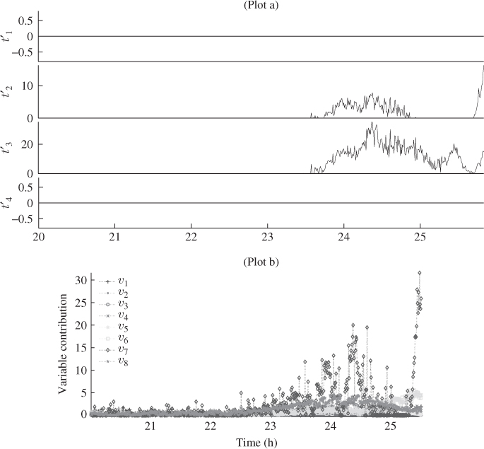
In plot (a) of Figure 5.15, a value of zero implies acceptance of the null hypothesis, that is, ![]() . Conversely, values larger than zero yield rejection of the null hypothesis. Plot (b) in Figure 5.15 shows the computed variable contribution by applying 3.38 and 3.39 for variables
. Conversely, values larger than zero yield rejection of the null hypothesis. Plot (b) in Figure 5.15 shows the computed variable contribution by applying 3.38 and 3.39 for variables ![]() and
and ![]() , and highlights that v7 (fresh feed flow) is most dominantly contributing.
, and highlights that v7 (fresh feed flow) is most dominantly contributing.
The second and severe drop developed over a period of 1 hour and resulted in an eventual reduction to just over 17![]() . According to Figure 5.14, the Qf statistic was sensitive around 25.5h into the data set, that is, before the fresh feed flow reached its bottom level. Around the same time, the Hotelling's T′2 statistic also increased sharply in value and with a slight delay, the Hotelling's T2 statistic violated its control limit.
. According to Figure 5.14, the Qf statistic was sensitive around 25.5h into the data set, that is, before the fresh feed flow reached its bottom level. Around the same time, the Hotelling's T′2 statistic also increased sharply in value and with a slight delay, the Hotelling's T2 statistic violated its control limit.
The preceding discussion outlined that the first drop did not have an effect on the C5 in C4 concentration, that is, the product quality. However, the prolonged drop in feed level from 25 to 24![]() is (relative to the variations in feed of the large reference data set) unusual and affected the second and third t′-score variables. This suggests that monitoring these two variables along with the most dominant contributor for product quality, the first t-score variable, is an effective way of detecting minor but prolonged drops in feed.
is (relative to the variations in feed of the large reference data set) unusual and affected the second and third t′-score variables. This suggests that monitoring these two variables along with the most dominant contributor for product quality, the first t-score variable, is an effective way of detecting minor but prolonged drops in feed.
Figure 5.16 shows the progression of the first drop using scatter diagrams in six stages. The first 23 hours and 20 minutes (2800 samples) are plotted in the upper left plot and indicate, as expected, that the scatter points cluster around the center of coordinate system. Each of the following plots, from the top right to the bottom right plot, adds 25 or 50 minutes of data and covers the additional range from 23 hours and 20 minutes to 25 hours and 50 minutes. Therefore, the bottom right plot describes the first stage of the second and sharp reduction in feed level.
Figure 5.16 Scatter diagrams for t1, ![]() and
and ![]() showing various stages in feed drop.
showing various stages in feed drop.
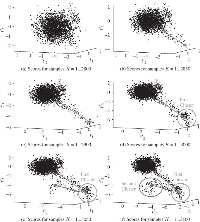
First, the scatter points move away from the initial cluster, which represents an in-statistical-control behavior, in the direction of the ![]() - and
- and ![]() -score variable and establishes a second cluster, which represents the first drop in feed. When the second and more severe drop in feed emerges, the scatter points move away from this second cluster and appear to establish a third cluster. It is interesting to note that this third cluster is shifted from the original one along the axis of the t1-score variable.
-score variable and establishes a second cluster, which represents the first drop in feed. When the second and more severe drop in feed emerges, the scatter points move away from this second cluster and appear to establish a third cluster. It is interesting to note that this third cluster is shifted from the original one along the axis of the t1-score variable.
Plot (a) in Figure 5.17 shows, graphically, the hypothesis test of 3.37 for each of the t-score variables, covering the second drop in feed. This time, as Figure 5.14 confirms, each monitoring statistic showed an out-of-statistical-control situation. Score variables t2 and t3 were initially most sensitive to the significant reduction in feed and after about 26 hours into the data set. Applying the procedure for determining the variable contributions in 3.38 and 3.39, on the basis of these score variables produced the plot (b) in Figure 5.17.
Figure 5.17 t scores and variable contributions to feed drop for 25 to 26 hours.
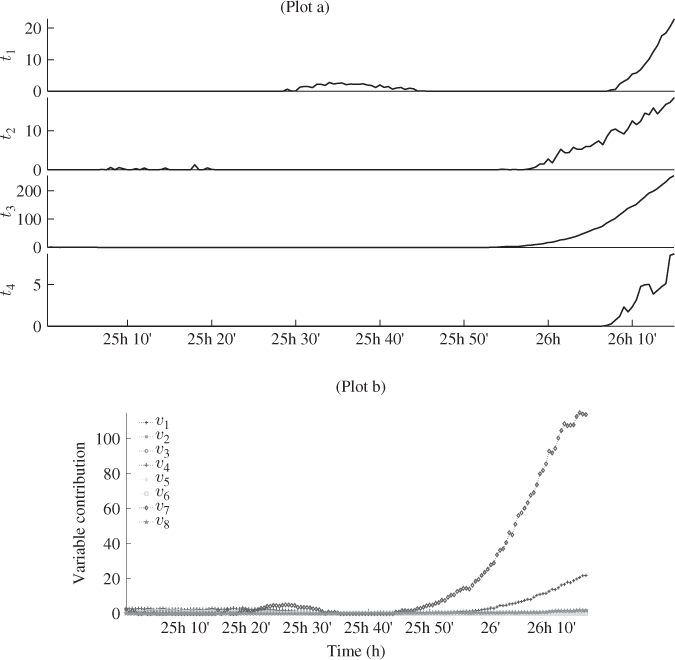
The main contributing variables to this event were the flow rate of the fresh feed v7 and with a delay the tray 14 temperature v1. Applying the same procedure for the first t-score variable between 25h and 30min and 25h and 50min (not shown here) yields the tray 14 temperature as the main contributor. This results from the sharply decreasing value of this variable during this period, which Figure 5.11 confirms.
Recall that the MRPLS monitoring model is a steady state representation of this unit that is based on modeling the correlation structure between the input and output variables but also among the input and output variable sets. The observed decrease in the tray 14 temperature is a result of the energy balance within the column that may not be described by the static correlation-based model. On the basis of an identified dynamic model of this process, Schubert et al. (2011) argued that the increase in the impurity level of the top draw (C5 in C4 concentration) originates from an upset in the energy balance. On the other hand, Buckley et al. (1985) pointed out that the flow rate of the fresh feed is the most likely disturbance upsetting the energy balance within the distillation column. Other but minor sources that may exhibit an undesired impact upon the energy balance is the fresh feed temperature and enthalpy.
In this regard, the application of the MRPLS monitoring model, however, correctly detected the reduction in feed level as the root cause triggering the undesired increase in the C5 in C4 concentration. Furthermore, the monitoring model was also capable of discriminating:
- between a minor reduction in feed level that was still abnormal relative to the reference data set but did not affect product quality; and
- a severe drop in this level that had a profound and undesired impact on product quality.
More precisely, the preceding analysis suggested that the t′-score variables and thus the Hotelling T′2 statistic reject the null hypothesis, that is, the process is in-statistical-control, if abnormal changes in the feed level arise. On the other hand, if such changes are significant, the t-score variables and with them the Hotelling's T2 and the Qf statistics reject the null hypothesis. This confirms the benefits of utilizing the model structure in 2.51. From the point of the process operator, the Hotelling's T2 and the Qf statistics are therefore informative, as they can provide an early warning that a feed drop has arisen that has the potential to affect produce quality. The immediate implementation of the recommendations in Meronk (2001) can prevent the negative impact of this change in feed level upon produce quality. For a minor alteration in feed level, however, is important to assess its duration as the prolonged presence may also have the potential to upset the energy balance.
1 To ensure an unbiased estimation, the denominator may not be assumed to be K − 1 given that the loading matrix and the scores are estimates too. With the large number of samples available, however, the estimate given in this equation is sufficiently accurate.