Chapter 8

Monitoring changes in covariance structure

Over the past decades, many successful MSPC application studies have been reported in the literature, for example Al-Ghazzawi and Lennox (2008); Aparisi (1998); Duchesne et al. (2002); Knutson (1988), Kourti and MacGregor (1995, 1996), Kruger et al. (2001), MacGregor et al. (1991), Marcon et al. (2005), Piovoso and Kosanovich (1992), Raich and Çinar (1996), Sohn et al. (2005), Tates et al. (1999), Veltkamp (1993), Wilson (2001). This chapter shows that the conventional MSPC framework, however, may be insensitive to certain fault conditions that affect the underlying geometric relationships of the LV sets. Section 8.1 demonstrates that even substantial alterations in the geometry of the sample projections may not yield acceptance of the alternative hypothesis that the process is out-of-statistical-control.

As the construction of the model and residuals subspaces as well as the control ellipses/ellipsoid for PCA/PLS models originate from data covariance and cross-covariance matrices, this problem is referred to as a change in covariance structure. Any change in these matrices consequently affects the orientation of these subspaces. Thus, in order to detect such alterations, it is imperative to monitor changes in the underlying data covariance structure, which Section 8.2 highlights. This section also presents preliminaries of the statistical local approach that allows constructing non-negative squared statistics that directly relate to the orientation of the model and residual subspaces and the control ellipses/ellipsoid.

This problem has been addressed by Ge et al. (2010, 2011), Kruger and Dimitriadis (2008); Kruger et al. (2007), and Kumar et al. (2002) by introducing a different paradigm to the MSPC-based framework. Blending the determination of the LV sets into the statistical local approach gives rise to the construction of statistics, which Section 8.3 introduces for PCA. These statistics are referred to as primary residuals that follow an unknown but non-Gaussian distribution.

It follows from the central limit theorem that a sum of random variables follow asymptotically a Gaussian distribution. This is taken advantage of in defining improved residuals that are based on the primary residuals. Section 8.4 revisits the simulation examples in Section 8.1 and shows that the deficiency of conventional MSPC can be overcome by deriving monitoring charts from the improved residuals.

Sections 8.5 introduces a fault diagnosis scheme to extract fault signatures for determining potential root causes of abnormal events. Section 8.6 applies the introduced monitoring approach to experimental data from a gearbox system. As in Section 8.4, the application study of the gearbox system highlights that the improved residuals are more sensitive in detecting abnormal process behavior when compared to conventional score variables.

Section 8.7 then discusses some theoretical aspects that stem from blending the statistical local approach into the conventional MSPC framework. This includes a direct comparison between the monitoring functions derived in Sections 8.3 and the score variables obtained by the PCA models and provides a detailed analysis the Hotelling's T² and Q statistics derived from the improved residuals. The chapter concludes in Section 8.8 with a tutorial session concerning the material covered, including questions as well as homework and project assignments.

8.1 Problem analysis

This section presents examples demonstrating that conventional MSPC-based process monitoring maybe insensitive to changes in the covariance structure of the process variables. A statistic, developed here, describes under which conditions traditional fault detection charts are insensitive to such changes. All stochastic variables in this section are assumed to be of zero mean, which, according to (2.2), implies that z = z₀. For simplicity, this section uses the data vector z instead of z₀.

8.1.1 First intuitive example

This example involves two process variables constructed from two i.d. source variables of zero mean, s₁ and s₂, which have a variance of σ₁² = 10 and σ₂² = 2. The following transformation describes the construction of the process variables

8.1

Here, T⁽⁰⁾ is a transformation matrix and the index (0) refers to the reference covariance structure. Equation (8.1) is an anticlockwise rotation of the original axes by 30°. Thus, and are coordinates of the rotated base, while s₁ and s₂ are coordinates of the original base. The covariance matrix of is

8.2

From (8.1), a total of 100 samples for and are generated. The plots in column (a) of Figure 8.1 show the corresponding scatter diagram (upper plot) and the Hotelling's T² statistic. The anticlockwise rotation can be noticed from the orientation of the ellipse. Moreover, the rotation does not affect the length of the semimajor and semiminor. For α = 0.01, , and the values of semimajor and semiminor are and , respectively. A detailed discussion on how to construct control ellipses is given in Subsection 1.2.3. Specifically designed changes in the covariance structure of and are carried out next in order to demonstrate that conventional MSPC may not be able to detect them.

8.1.1.1 First change in covariance structure

The following transformation changes the covariance structure between and

8.3

where T⁽¹⁾ describes an anticlockwise rotation by 45° and the index (1) refers to the first change. Consequently, T⁽¹⁾T⁽⁰⁾ first represents an anticlockwise rotation by 30° to produce z⁽⁰⁾ and a subsequent rotation by 45° to determine z⁽¹⁾. The variables z⁽¹⁾ are the coordinates to a base that is rotated by 75° relative to the original cartesian base. The covariance matrix for z⁽¹⁾, , is

8.4

Using (8.3), a total of 100 samples are generated for z⁽¹⁾. From this set, the column plots associated with (b) in Figure 8.1 show the scatter diagram (upper plot) and the Hotelling's T² statistic (lower plot). For the scatter diagram, the dashed and solid lines represent the control ellipse for the variable sets z⁽¹⁾ and z⁽⁰⁾, respectively. Furthermore, the Hotelling's T² statistic for each sample is computed with respect to . Since eight points fall outside the confidence regions for the scatter diagram and the control limit of the Hotelling's T² statistic, the charts correctly indicate an out-of-statistical-control situation. Consequently, this change in covariance structure between and is identifiable.

8.1.1.2 Second change in covariance structure

The same experiment is now repeated, but this time the variance of the i.d. sequences s₁ and s₂ is σ₁ = 3 and , respectively. Applying (8.3) to first produce and and subsequently and gives rise to the covariance matrix

8.5

With the reduced variance for s₁ and s₂, 100 samples are generated using (8.3). The plots in column (c) of Figure 8.1 show the scatter diagram of and and the Hotelling's T² statistic based on . The dashed control ellipse corresponds to and and the solid one refers to and . Despite significant alterations to the covariance structure of and these changes are undetected since the dashed control ellipse is inside the solid one. Therefore, the alteration renders the scatter diagrams and the Hotelling's T² statistic blind.

In essence, if changes to the covariance structure arise that lead to small alterations in the geometry of statistical confidence regions and limits, such events may not be detectable. Next, a more detailed statistical analysis is presented to formulate conditions which render conventional multivariate analysis insensitive.

8.1.2 Generic statistical analysis

The intuitive analysis in the previous subsection suggested that changes in the covariance structure manifest themselves in alterations of the eigenvalues and eigenvectors of the covariance matrix. This follows from (8.2), (8.4) and (8.5). However, this analysis was restricted to rotations of the control ellipse and is therefore limited in a multivariate context. More precisely, since MSPC techniques decompose the data space(s) into model and residual subspaces, a more generic condition must to be developed to investigate whether the above insensitivity can generally arise.

Concentrating on the non-negative quadratic Hotelling's T² and Q statistics, violations of their control limits are indicative of such changes. This postulates the following condition for changes in the covariance structure to be undetectable.

This represents a condition that can be satisfied by examining the control limits of the non-negative quadratic statistics. Subsection 3.1.2 showed that the control limit of the Hotelling's T² statistic is, asymptotically, the critical value of a χ² distribution for the significance α. On the other hand, the control limit of the Q statistic can be approximated by a χ² distribution (Box 1954; Jackson and Mudholkar 1979; MacGregor and Kourti 1995; Satterthwaite 1941). With this in mind, it follows that

8.6

where η and θ are a weight factor and the number of degrees of freedom of a χ² distribution, respectively. It should be noted that the approximation in (8.6) is also applicable to the Hotelling's T² statistic.

In the case of PCA,

• is the ith largest eigenvalue of S_zz, and m₀ and m₁ are 1 and n, respectively, for the Hotelling's T² statistic; and
• , and m₀ and m₁ are n + 1 and n_z, respectively, for the Q statistic.

For PLS,

• is , and m₀ and m₁ are 1 and n, respectively, for the Hotelling's T² statistic; and
• , and m₀ and m₁ are n + 1 and n_x, respectively, for the Q_e statistic.

Although the relationship below is also applicable to the Q_f statistic for PLS, this analysis is not considered here.

Estimating the sample mean and variance of the sequence , , ···  , , (3.30) and (3.31) show that

8.7

if K₀ is sufficiently large. Here, the sub- and superscript (0) refer, as before, to the reference condition, and and are the estimated mean and variance, respectively. For a second sequence, , which contains a total of K₁ samples , , ···  , , describing a change in the variable covariance structure, the parameters and can be obtained. Here, the sub- and superscript (1) refer to the second operating condition. Using the estimates , , and allows formulating the following condition for detecting the second and abnormal operating condition.

Under the application of above condition, score-based process monitoring using conventional MSPC may be insensitive to changes in the variable covariance structure, which the next subsection illustrates using a three-variable example.

8.1.3 Second intuitive example

The three variables are defined by a linear combination of the two zero mean i.d. source signals and , which have a variance of and . As before, the superscript ⁽⁰⁾ refers to the original covariance structure. According to (2.2), the zero mean error vector , augmented to the common cause variation Ξs⁽⁰⁾, has an error covariance matrix . Furthermore, (8.8) defines the score and loading vectors for the data vector .

8.8

The matrix T⁽⁰⁾ stores the eigenvectors of and is a vector storing the score variables. Under the assumption that , the covariance matrix of z⁽⁰⁾, , is equal to

8.9

which follows from (6.5). Moreover, the column space of Ξ is equal to the first two column vectors of T⁽⁰⁾. For simplicity, is assumed here that Ξ contains these column vectors, implying that the orthogonal complement, , is the transpose of the third column vector and the generalized inverse, Ξ^†, is the transpose of Ξ.

The contribution of the first, second and third principal components to the sum of the variances of the three process variables are , and , which follows from (2.116) to (2.122). Equation (6.73) highlights that the first two score variables mainly describe the two source variables, which contribute 97.94% to this sum of variances, whilst the contribution of the third score variable is 2.04% and, according to (3.7), relates to .

The eigenvectors and span the model subspace and spans the residual subspace. As the data space corresponding to z₁, z₂ and z₃ is a Cartesian space, the minimum angles of the axes z₁, z₂ and z₃ to the third eigenvector are 54.74°, 54.74° and 125.26°, respectively. The critical value of a χ² distribution for two degrees of freedom and α = 0.01 is . The lengths of the semimajor and semiminor of the control ellipse (first two score variables) are, therefore, and , respectively, λ₁ = 16 and λ₂ = 8.

To introduce alterations to this data covariance structure and to examine whether these alterations are detectable, a total of four changes are considered. Each of these changes relates to an anticlockwise rotation of the original variable set by 30°. Equation (8.10) shows the corresponding rotation matrix T⁽¹⁾

8.10

The first change is a simple rotation of the first two variables

8.11

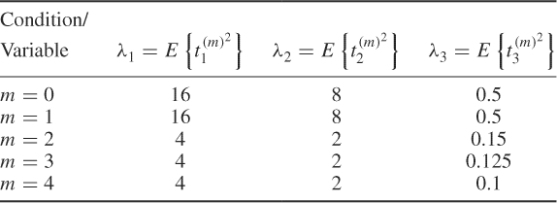
where . The remaining three changes also alter the variance of the score variables, listed in Table 8.1, which produces the data vectors z⁽²⁾, z⁽³⁾ and z⁽⁴⁾

8.12

There are now the following five variable sets:

To demonstrate how different these five variable sets are requires the inspection of the corresponding covariance matrices for z⁽⁰⁾, z⁽¹⁾, z⁽²⁾, z⁽³⁾ and z⁽⁴⁾

8.13

Table 8.1 Variance of score variables , and .

The next step is to perform a total of 1000 Monte Carlo simulations for each of the five variable sets, z⁽⁰⁾, ···  , z⁽⁴⁾. According to Condition 8.1.2, the changes in the covariance structure cannot be detected if the control limits associated with the variable sets representing z⁽¹⁾, z⁽²⁾, z⁽³⁾ and z⁽⁴⁾ are smaller or equal to the control limit corresponding to z⁽⁰⁾. It is important to note, however, that the non-negative quadratic statistics must be constructed from the PCA model related to the variable set z⁽⁰⁾. The calculation of the score variables for each of the five variable sets is

8.14

Based on (8.14), the five Hotelling's T² statistics are now constructed from the first two elements of the score vectors , ···  , and the score covariance matrix . The Q statistics are simply the squared values of the third elements of , ···  , . Each of the 1000 Monte-Carlo simulation experiments include a total of K = 100 samples. This gives rise to a total of 1000 estimates for the control limits of the Hotelling's T² and Q statistics for z⁽⁰⁾, …  , z⁽⁴⁾. To assess the sensitivity in detecting each of the four changes, the 2.5 and the 97.5 percentiles as well as the median can be utilized.

Figure 8.2 (a) shows the range limited by the 2.5 and 97.5 percentiles of the control limit for each of the five Hotelling's T² statistics , ···  , . Plot (b) in this figure shows the ranges for the control limits of , ···  , . The circle inside each of the ranges represents the median. Examining the range for the Hotelling's T² statistic in relation to Condition 8.1.2, it is clear that the Hotelling's T² statistic is insensitive to any of the changes introduced to the original covariance structure.

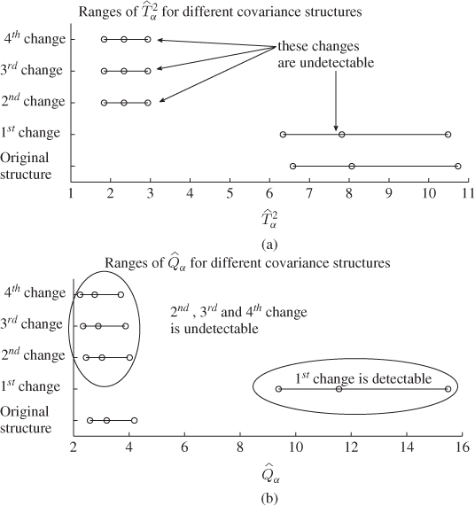
A different picture emerges when making the same comparison for the Q statistic. While the range for covers values between 2.2 and 4 (roughly), the values for range between around 9.5 and 15.5.¹ According to Condition 8.1.2, this implies that this first alteration is detectable by the Q statistic. In contrast, the remaining three changes may not be detectable as the ranges for , and have a significant overlap with the range for . More precisely, the 2.5 and 97.5 percentiles for are larger than those for , and . Consequently, the second to fourth alterations are not detectable by the Hotelling's T² and may not be detectable by the Q statistic either.

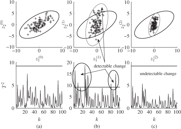
To graphically illustrate the above findings, a total of 100 samples are generated for variable sets z⁽⁰⁾, z⁽¹⁾ and z⁽²⁾. Referring to these sets as data set 1, data set 2 and data set 3, corresponding to z⁽⁰⁾, z⁽¹⁾ and z⁽²⁾, respectively, Figure 8.3 shows the results of analyzing them using a PCA model established from data set 1. In this figure, the column in rows (a), (b) and (c) represent the analysis of data set 1, data set 2 and data set 3, respectively. The upper plots show the control ellipse and the scatter plots of data sets 1 to 3. The plots in the middle and lower row of Figure 8.3 present the Hotelling's T² and the Q statistics, respectively.

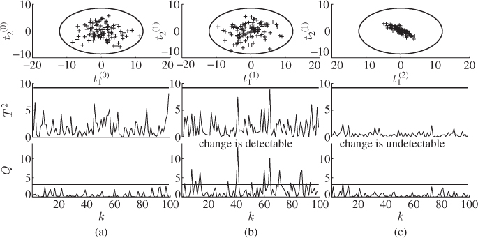
The plots associated with index (a) indicate that the projection of each of the 100 samples of data set 1 onto the model subspace fall inside the control ellipse. This, in turn, implies that none of the samples results in a violation of the control limit of the Hotelling's T² statistic. Also the residual Q statistic has not violated its control limit, Q_0.01 = 3.2929, for any of the 100 samples of data set 1. Hence, the hypothesis that the process is in-statistical-control must be accepted.

A different result emerges when inspecting the plots associated with data set 2, representing an anticlockwise rotation of z₁ − z₂ axis by 30°. Although projecting the samples onto the model subspace shows no projections outside the control ellipse, the Q statistic highlights that the squared distance of a total of 16 samples from the model subspace is larger than 3.2929. This change is therefore detectable.

Finally, the plots corresponding to data set 3 point out that the projected samples onto the model subspace fall inside the control ellipse and that the squared distance of each sample from the model subspace is less than 3.2929. Consequently, this change remains undetected, which is undesirable. The remainder of this chapter describes the incorporation of the statistical local approach into the MSPC framework to detect such changes.

With regards to the second, third and fourth alterations, one could justifiably argue that if the third eigenvalue is not changed from 0.5 to 0.15, 0.125 and 0.1, respectively, any of these changes are detectable by the Q statistic. This follows from (6.4) and (6.5), which highlight that λ₃ corresponds to the noise variance. According to Figure 8.3, the rotation of the control ellipse changes its orientation relative to the original model subspace. Thus, samples that are further away from the center of the ellipse but still inside produce a larger distance to the original model subspace.

If the axes of the rotated control ellipse are linear combinations of the eigenvectors spanning the model subspace, the rotated ellipse remains inside the model subspace. Hence, such an alteration of the covariance structure has no effect on the residual subspace and hence the Q statistic. Revisiting the geometric analysis in Figure 8.1, a change in the orientation and dimension may yield a control ellipse that lies within the original ellipse and is on the model subspace. Equations (6.7) to (6.11) outline that such an alteration results from a change in the covariance matrix of the source signals and may, consequently, remain undetected.

8.2 Preliminary discussion of related techniques

After outlining that the basic MSPC monitoring framework may not detect certain changes in the data covariance structure, a different paradigm is required to address this issue. Revisiting the analysis in Figure 8.1, the exact shape and orientation of a control ellipse is defined by the eigenvectors and eigenvalues of . In other words, if the orientation of the eigenvectors and the eigenvalues could be monitored on-line, any change in the covariance structure can consequently not go unnoticed. It is therefore required to formulate monitoring functions that directly relate to the eigen decomposition of .

Basseville (1988) described a statistical theory, known as the statistical local approach, that can be readily utilized to define vector-valued monitoring functions, referred to as primary residual vectors , of the form

8.15

where is a vector of model parameters and . For simplicity, the distribution function of is assumed to be unknown at this point.

The parameter vectors includes the eigendecomposition of for PCA and and for PLS. The construction of the primary residuals for PCA is discussed in Sections 8.3. For a statistical inference based on , however, the following problem arises. How to construct a monitoring framework if cannot be assumed to be Gaussian or is unknown, as assumed thus far?

This question can be answered by assuming that z₀ stores i.i.d. sequences, that is, , where k and l are sample indices. As the distribution function of depends on the distribution function of z₀, instances of are also i.i.d. Under these conditions, the following sum of the primary residual vectors

8.16

follows, asymptotically, a Gaussian distribution function, which is a result of the CLT. Subsection 8.7.1 provides a detailed discussion and a proof of the CLT. The sum in (8.16) is defined as the improved residual vector and is, asymptotically, Gaussian distribution. If and , and can be utilized to construct scatter diagrams as well as a Hotelling's T² statistic as discussed in Subsection 3.1.2.

For PCA, it is sufficient to develop primary residuals related to the eigenvalues and the eigenvectors of , as they determine the orientation of the model and the residual subspaces, and the size and orientation of the control ellipse. For PLS, however, there are two interrelated data spaces. Project 2 in the tutorial session of this chapter extends the development of improved and primary residuals for PLS.

For PCA, the next section discuss the construction of primary and improved residuals describing changes in the geometry of the model and residual subspaces and summarizes their basic statistical properties.

8.3 Definition of primary and improved residuals

Sections 2.1 and 9.3 outline that a PCA monitoring model is completely described by the eigendecomposition of . This includes the orientation of the model and residual subspaces as well as the orientation and size of the n dimensional control ellipsoid. Consequently, the primary residuals rely on the eigendecomposition of , and are derived in Subsection 8.3.1 using the definition of the ith eigenvector . Subsection 8.3.2 shows that primary residuals can also be obtained from . Subsections 8.3.3 and 8.3.4 contrast both types of primary residuals and determine their statistical properties. Finally, Subsection 8.3.5 shows the construction of improved residuals.

8.3.1 Primary residuals for eigenvectors

Starting with the definition of the objective function for obtaining the ith eigenvector

8.17

the partial derivative of (8.17) allows determining the optimal solution

8.18

which is given by

8.19

The above equation relies on the fact that . Now, defining

8.20

allows simplifying Equation (8.19) to become

8.21

and consequently

8.22

It follows from (8.22) that in the vicinity of p_i, defined by for which , the following holds true

8.23

Equations (8.22) and (8.23) imply that each loading vector p_i produces a corresponding statistic such that , when p is the equal to the ith eigenvector of . In contrast, any deviation from zero indicates that p_i is no longer the eigenvector associated with the ith eigenvalue.

The next step is to define two parameter vectors that store the eigenvectors spanning the model and residual subspaces. The vector for the model subspace, , is

8.24

and that of the residual subspace, , is defined as

8.25

This gives rise to the following two primary residual vectors for the model subspace

8.26

and the residual subspace

8.27

The next subsection develops primary residual vectors for the eigenvalues of .

8.3.2 Primary residuals for eigenvalues

Pre-multiplying (8.20) by gives rise to

8.28

The expectation of directly follows from (8.22)

8.29

As before, defines the neighborhood of λ_i, where . This implies that holds true if and only if λ is the ith largest eigenvalue of . In a similar fashion to the and , and and , and , and and , for the retained and discarded eigenvalues can be defined as follows

8.30

The next subsection provides a detailed examination of the primary residuals.

8.3.3 Comparing both types of primary residuals

The analysis concentrates first on the primary residual vectors and , which have the dimension n_zn and n_z(n_z − n), respectively. These dimensions, therefore, depend on the ratio . If n is close to n_z or if n is small compared to n_z, the size of or can be substantial. This subsection then compares the sensitivity of and , with and for detecting changes in the covariance structure.

8.3.3.1 Degrees of freedom for primary residuals and

A closer inspection of the primary residuals and reveals that its elements may be linearly dependent. This is best demonstrated by a joint analysis

8.31

which can alternatively be written as

8.32

In matrix-vector form, (8.32) becomes

8.33

Since has full column rank, its rank is equal to . More precisely, a total of elements in the combined primary residual vector are linearly dependent upon the remaining ones.

For the primary residual vectors and , this has the following consequence: if the number of the elements in:

• and
• 

is larger than or equal to

there is a linear dependency between these primary residuals. This gives rise to linear dependency among the elements in and under the following conditions

and leads to the following criteria for

8.34

and

8.35

From the above relationships, it follows that

8.36

which can only be satisfied if if n_z is even and if n_z is odd. Figure 8.4 summarizes the above findings and shows graphically which condition leads to a linear dependency of the primary residuals in and .

The importance of these findings relates to the construction of the primary residual vectors, since the number of source signals is determined as part of the identification of a principal component model. In other words, the original size of and is n_zn and n_z(n_z − n), respectively, and known a priori. If the analysis summarized in Figure 8.4 reveals that elements stored in the primary residual vectors are linearly dependent, the redundancy can be removed by eliminating redundant elements in or , such that this number is smaller or equal to in both vectors.

8.3.3.2 Sensitivity analysis for , , and

To investigate whether the primary residuals and can both detect changes in the eigenvalues and the eigenvectors of , the examination focuses on:

• the primary residuals and to evaluate their sensitivity in detecting changes in the eigenvectors and eigenvalues associated with the orientation of the model subspace and the orientation and size of the control ellipsoid; and
• the primary residuals and to examine their sensitivity in detecting changes in the eigenvectors and eigenvalues related to the orientation of the residual subspace and, according to (3.16), the approximation of the distribution function of the sum of squared residuals.

The resultant analysis yields the following two lemmas, which are proved below.

 

 

Directional changes of the ith eigenvector

Assuming that λ_i remains unchanged, (8.19) can be rewritten on the basis of (8.37)

8.38

Knowing that a change in the covariance structure between the recorded process variables produces a different , denoted here by , (8.38) becomes

8.39

The expectation of the primary residual vector and given by

8.40

It follows that depends on the changes of the elements in . Equation (8.40) shows that the condition only arises if and only if p_i is also an eigenvector of associated with λ_i. This situation, however, cannot arise for all 1 ≤ i ≤ n_z unless . An important question is whether the primary residual also reflect a directional changes of p_i. This can be examined by subtracting from (8.39), where is the eigenvector of associated with λ_i, which yields

8.41

Pre-multiplying the above equation by produces

8.42

It is important to note that if the pre-multiplication is carried out by the transpose of , (8.42) becomes zero, since . Consequently, any directional change of p_i manifests itself in . This, in turn, implies that both primary residual vectors, and , are sufficient in detecting any directional change in p_i by a mean different from zero. It should also be noted that if if both vectors are orthogonal to each other. A closer inspection of (8.42), however, yields that only the trivial case of can produce ϵ_i = 0.

Changes in the ith eigenvalue

Now, λ_i changes under the assumption that p_i remains constant. For this change, (8.39) becomes

8.43

Subtracting , based on the correct eigenvalue , from Equation (8.43) gives rise to

8.44

and hence, , which implies that is sensitive to the change in λ_i. Finally, pre-multiplication of (8.44) by yields

8.45

where . Thus, . This analysis highlights that both primary residual vectors, and , can detect the change in λ_i.

The above lemmas outline that any change in the covariance structure of z₀ can be detected by and ϕ_i. Given that:

• the dimensions of the primary residuals and are significantly smaller than those of and , respectively;
• the primary residuals for the eigenvectors and the eigenvalues, and , can detect a change in the covariance structure of z₀; and
• the elements in the primary residual vectors and cannot generally be assumed to be linearly independent,

it is advisable to utilize the primary residual vectors and for process monitoring. For simplicity, the parameter vectors are now denoted as follows and . Moreover, the tilde used to discriminate between and its scaled sum is no longer required and can be omitted. The next subsection analyzes the statistical properties of and .

8.3.4 Statistical properties of primary residuals

According to (8.29), the expectation of both primary residual vectors, and , is equal to zero. The remaining statistical properties of ϕ_i include its variance, the covariance of ϕ_i and ϕ_j, the distribution function of ϕ_i and the central moments of ϕ_i. This allows constructing the covariance matrices for and , and , respectively.

Variance of ϕ_i

The variance of ϕ_i can be obtained as follows:

8.46

which can be simplified to

8.47

Given that:

• ; and
• 

it follows that . As t_i is Gaussian distributed, central moments of are 0 if m is odd and . If m is even.² For m = 2, and for m = 4, . Substituting this into (8.47) gives rise to

8.48

Covariance of ϕ_i and ϕ_j

The covariance between two primary residuals is

8.49

and can be simplified to

8.50

Now, substituting , and , which follows from the Isserlis theorem (Isserlis 1918) and the fact that t_i and t_j are statistically independent and Gaussian distributed, (8.50) reduces to

8.51

Consequently, there is no covariance between ϕ_i and ϕ_j, implying that the covariance matrices for and reduce to diagonal matrices.

Distribution function of ϕ_i

The random variable

8.52

yields the following distribution function

8.53

since . In other words, the distribution function of ϕ_i can be obtained by substituting the transformation in (8.52) into the distribution function of a χ² distribution with one degree of freedom

8.54

which gives rise to

8.55

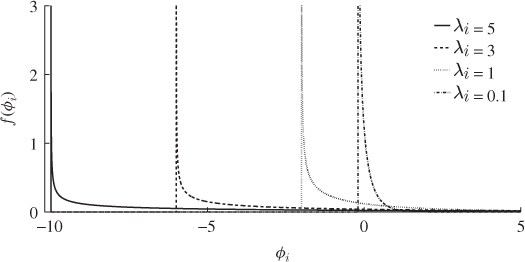
With respect to (8.55), the PDF f(ϕ_i) > 0 within the interval ( − 2λ_i, ∞), which follows from the fact that . In (8.54) and (8.55), Γ(1/2) is the gamma function, defined by the improper integral . Figure 8.5 shows the probability density function of the primary residuals for various values of λ_i. The vertical lines in this figure represent the asymptotes at − 2λ_i.

Central moments of ϕ_i

The determination of the central moments of ϕ_i relies on evaluating the definition for central moments, which is given by

8.56

According to (8.56), the central moments can be obtained directly by evaluating the expectation , which gives rise to

8.57

Isolating the terms in (8.57) that are associated with and substituting the central moments for yields

8.58

where

8.59

are binomial coefficients and m! = 1 · 2 · 3 ··· (m − 1) · m. Table 8.2 summarizes the first seven central moments of ϕ_i.

Table 8.2 First seven central moments of ϕ_i.

Order m	Central moment
1	0
2
3
4
5
6
7

8.3.5 Improved residuals for eigenvalues

Equation (8.16) shows that the improved residuals are time-based sums of the primary residuals and asymptotically Gaussian distributed, given that the primary residuals are i.i.d. sequences. Following from the geometric analysis of the data structure and its assumptions, discussed in Subsection 2.1.1, the model and residual subspaces are spanned by the n dominant and the remaining n_z − n eigenvectors of , respectively.

Using the definition of the primary residuals for the eigenvalues, the improved residuals become

8.60

As the eigenvectors and eigenvalues are functions of , the dependencies on these parameters can be removed from (8.16) and hence, θ_i = θ_i(z₀, K) with K being the number of samples and ϕ_i = ϕ_i(z₀(k)). The first and second order moments of θ_i(z₀, K) are as follows

8.61

and

8.62

respectively. Note that the factor 2 in (8.28) has been removed, as it is only a scaling factor. The variance of ϕ_i is therefore . That follows from the Isserlis theorem (Isserlis 1918). The improved residuals can now be utilized in defining non-negative quadratic statistics.

The separation of the data space into the model and residual subspaces yielded two non-negative quadratic statistics. These describe the variation of the sample projections onto the model subspace (Hotelling's T² statistic) and onto the residual subspace (Q statistic). With this in mind, the primary residuals associated with the n largest eigenvalues and remaining n_z − n identical eigenvalues can be used to construct the Hotelling's T² and residual Q statistics, respectively.

Intuitively, the definition of these statistics is given by

8.63

and follows the definition of the conventional Hotelling's T² and Q statistics in (3.8) and (3.15), respectively.

As the number of recorded samples, K, grows so does the upper summation index in (8.60). This, however, presents the following problem. A large K may dilute the impact of a fault upon the sum in (8.60) if only the last few samples describe the abnormal condition. As advocated in Chapter 7, however, this issue can be addressed by considering samples that are inside a sliding window only. Defining the window size by k₀, the incorporation of a moving window yields the following formulation of (8.60)

8.64

The selection of k₀ is a trade-off between accuracy and sensitivity. The improved residuals converge asymptotically to a Gaussian distribution, which demands larger values for k₀. On the other hand, a large k₀ value may dilute the impact of a fault condition and yield a larger average run length, which is the time it takes to detect a fault from its first occurrence. The selection of k₀ is discussed in the next section, which revisits the simulation examples in Section 8.1.

8.4 Revisiting the simulation examples of Section 8.1

This section revisits both examples in Section 8.1, which were used to demonstrate that the conventional MSPC framework may not detect changes in the underlying covariance structure.

8.4.1 First simulation example

Figure 8.1 showed that the scatter diagram and the Hotelling's T² statistic only detected the first change but not the second one. Recall that both changes resulted in a rotation of the control ellipse for and by 45°. Whilst the variance of both score variables remained unchanged, the variances for the second change were significantly reduced such that the rotated control ellipse was inside the original one.

Given that both changes yield a different eigendecomposition for the variable pairs , and , , the primary residuals are expected to have a mean different from zero. Before determining improved residuals, however, k₀ needs to be determined. If k₀ is too small the improved residuals may not follow a Gaussian distribution accurately, and a too large k₀ may compromise the sensitivity in detecting slowly developing faults (Kruger and Dimitriadis 2008; Kruger et al. 2007).

Although the transformation matrix T⁽⁰⁾ and the variances of the i.d. score variables and are known here, the covariance matrix and its eigendecomposition would need to be estimated in practice. Table 8.3 summarizes the results of estimating the covariance of both improved residual variables for a variety of sample sizes and window lengths.

Table 8.3 Estimated means and variances of improved residuals

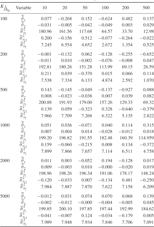
As per their definition, the improved residuals asymptotically follow a Gaussian distribution of zero mean and variance if the constant term in (8.28) is not considered. The mean and variance for θ₁ and θ₂ are 2 × 10² = 200 and 2 × 2² = 8, respectively. The covariance E{θ₁θ₂} = 0 is also estimated in Table 8.3.

The entries in this table are averaged values for 1000 Monte Carlo simulations. In other words, for each combination of K and k₀ a total of 1000 data sets are simulated and the mean, variance and covariance values for each set are the averaged estimates. The averages of each combination indicate that the main effect for an accurate estimation is K, the number of reference samples of θ₁ and θ₂. Particularly window sizes above 50 require sample sizes of 2000 or above to be accurate.

This is in line with expectation, following the discussion in Section 6.4. The entries in Table 8.3 suggest that the number of reference samples for θ₁ and θ₂, K, need to be at least 50 times larger then the window size k₀. Another important issue is to determine how large k₀ needs to be to accurately follow a Gaussian distribution. Figure 8.6 shows Gaussian distribution functions in comparison with the estimated distribution functions of ϕ₁ and ϕ₂, and θ₁ and θ₂ for k₀ = 10, 50 and 200.

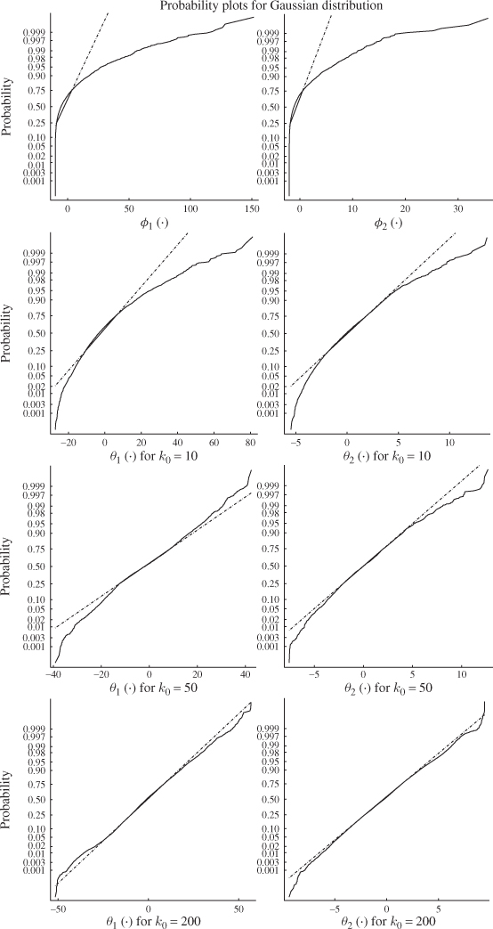
As expected, the upper plot in this figure shows that the distribution function of primary residuals depart substantially from a Gaussian distribution (straight line). In fact, (8.55) and Figure 8.5 outline that they follow a central χ² distribution. The plots in the second, third and bottom row, however, confirm that the sum of the primary residuals converge to a Gaussian distribution.

Whilst the smaller window sizes of k₀ = 10 and k₀ = 50 still resulted in significant departures from the Gaussian distribution, k₀ = 200 produced a close approximation of the Gaussian distribution. Together with the analysis of Table 8.3, a window size of k₀ = 200 would require a total of K = 200 × 50 = 10 000 reference samples to ensure that the variance of θ₁ and θ₂ are close to 2 λ₁² and 2 λ₂², respectively.

Using the same 1000 Monte Carlo simulations to obtain the average values in Table 8.3 yields an average of 200.28 and 7.865 for and , respectively, and − 0.243 for . After determining an appropriate value for k₀, the Hotelling's statistics can now be be computed as shown in (8.60).

Figure 8.7 compares the conventional Hotelling's T² statistic with the one generated by the statistical local approach. For k₀ = 200, both plots in this figure show a total of 100 samples obtained from the original covariance structure (left portion), the first change (middle portion) and the second change (right portion of the plots).

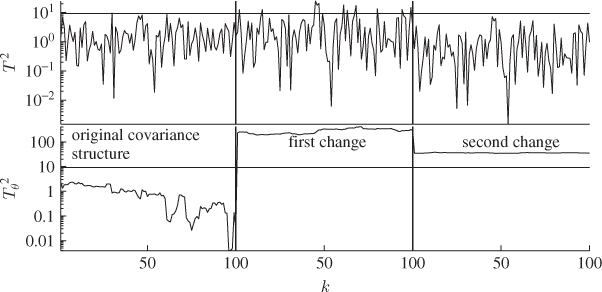
As observed in Figure 8.1, the conventional Hotelling's T² statistic could only detect the first change but not the second one. In contrast, the non-negative quadratic statistic based on the statistical local approach is capable of detecting both changes. More precisely, the change in the direction of both eigenvectors (first change) and both eigenvectors and eigenvalues (second change) yields an expectation for both primary residual function that is different from 0.

8.4.2 Second simulation example

Figures 8.2 and 8.3 highlight that conventional MSPC can only detect one out of the four changes of the original covariance structure. The remaining ones, although major, may not be detectable. Each of these changes alter the orientation of the model and residual subspaces as well as the orientation of the control ellipse. This, in turn, also yields a different eigendecomposition in each of the four cases compared to the eigendecomposition of the original covariance structure.

The primary residuals are therefore expected to have mean values that differ from zero. The first step is to determine an appropriate value for k₀. Assuming that the variances for each of the improved residuals, , and , need to be estimated, the same analysis as in Table 8.3 yields that K should be 100 times larger than k₀.

Figure 8.8 compares the estimated distribution function of the improved residuals with a Gaussian distribution function (straight lines) for different values of k₀. The estimation of each distribution function was based on K = 100 × 200 = 20 000 samples. As the primary residuals are χ² distributed the approximated distribution function, consequently, showed no resemblance to a Gaussian one. For k₀ = 10 and k₀ = 50, the estimated distribution function still showed significant departures from a Gaussian distribution. Selection k₀ = 200, however, produced a distribution function that is close to a Gaussian one.

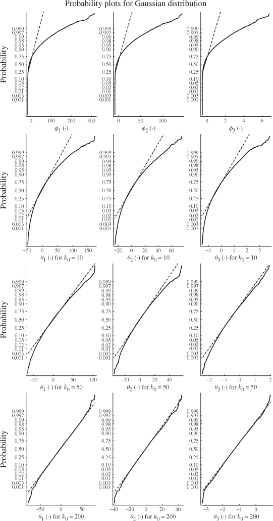
This is expected, as the improved residuals are asymptotically Gaussian distributed. In other words, the larger k₀ the closer the distribution function is to a Gaussian one. It is important to note, however, that if k₀ is selected too large it may dilute the impact of a fault condition and render it more difficult to detect. With this in mind, the selection of k₀ = 200 presents a compromise between accuracy of the improved residuals and the average run length for detecting an incipient fault condition.

Figure 8.9 contrasts the conventional non-negative quadratic statistics (upper plots) with those based on the statistical local approach (lower plots) for a total of 100 simulated samples. This comparison confirms that the Hotelling's T² and Q statistics can only detect the first change but are insensitive to the remaining three alterations.

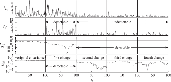
The non-negative quadratic statistics relating to the statistical local approach, however, detect each change. It is interesting to note that the first change only affected the Q_θ statistic, whilst the impact of the remaining three changes manifested themselves in the Hotelling's statistic. This is not surprising, however, given that the primary residuals are a centered measure of variance, which follows from (8.28).

To explain this, the variance of the three score variables can be estimated for each covariance structure. Determining the score variables as , where P stores the eigenvectors of , allows us to estimate these variances. Using a Monte Carlo simulation including 1000 runs, Table 8.4 lists the average values of the estimated variances. The Monte Carlo simulations for each of the five covariance structures were based on a sample size of K = 1000.

Table 8.4 Estimated variances of , and .

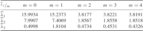
The sensitivity of the Hotelling's and Q_θ statistics for each alternation follows from the estimated averages in this table. The initial 30° rotation produces slightly similar variances for the first and second principal component. The variance of the third principal component, however, is about three and a half times larger after the rotation. Consequently, the Hotelling's statistic is only marginally affected by the rotation, whereas a very significant significant impact arises for the Q_θ statistic.

In contrast, the average eigenvalue for the second, third and fourth alteration produced averaged first and second eigenvalues that are around one quarter of the original ones. The averaged third eigenvalue, however, is very similar to the original one. This explains why these alterations are detectable by the Hotelling's statistic, while the Q_θ statistic does not show any significant response.

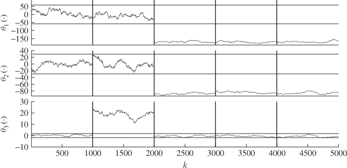
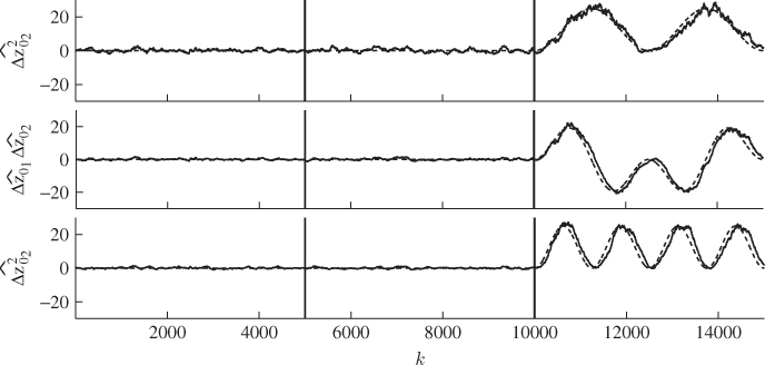
Plotting the improved residuals for each covariance structure and K = 1000, which Figure 8.10 shows, also confirms these findings. For a significance of 0.01, the control limits for each improved residual are . The larger variance of the third score variable yielded a positive primary residual for the first alteration. Moreover, the smaller variances of the first and second score variables produced negative primary residuals for the remaining changes.

8.5 Fault isolation and identification

For describing a fault condition, Kruger and Dimitriadis (2008) introduced a fault diagnosis approach that extracts the fault signature from the primary residuals. The fault signature can take the form of a simple step-type fault, such as a sensor bias that produces a constant offset, or can have a general deterministic function. For simplicity, the relationship of this diagnosis scheme concentrate first on step-type faults in Subsection 8.5.1. Subsection 8.5.2 then expands this concept to approximate a general deterministic fault signature.

8.5.1 Diagnosis of step-type fault conditions

The augmented data structure to describe a step-type follows from (3.68)

8.65

where represents an offset term that describes the fault condition. In analogy to the projection-based variable reconstruction approach, the offset can be expressed as follows

8.66

Here, is the fault direction and μ is the fault magnitude. With respect to the convention introduced by Isermann and Ballé (1997), the detection of a fault condition and the estimation of refers to fault isolation. As μ describes the size of the fault, the estimation of the fault magnitude represents the fault identification step.

Equation (8.67) describes the impact of the offset term upon the primary residual vector for the ith eigenvector

8.67

for omitting the constant of 2 in (8.20). Substituting (8.65) into (8.67) yields

8.68

Given that E{ϕ_i} = 0, E{z₀} = 0 and E{t_i} = 0, taking the expectation of (8.86) gives rise to

8.69

Here ⊗ refers to the Kronecker product of two matrices. The results of the two Kronecker products are as follows

8.70a

8.70b

With , (8.69) has a total of unknowns but only n_z linearly independent equations and is hence an underdetermined system. However, there are a total of n_z equations for 1 ≤ i ≤ n_z. Hence, (8.69) in augmented form becomes

8.71

It is interesting to note that the linear dependency in (8.69) and (8.71) follows from the analysis in Subsection 8.3.3 and particularly (8.33). It is therefore possible to remove the redundant column vectors of Ψ and elements of the vector ζ, which gives rise to

8.72

where and . The expectation on the left hand side of (8.72) can be estimated from the recorded data and the matrix Ψ_red is made up of the elements of loading vectors and hence known. The elements of the vector ζ_red are consequently the only unknown and can be estimated by the generalized inverse of Ψ_red, i.e.

8.73

For estimating , however, it is possible to rely on the improved residuals, since

8.74

Here, and Φ_f(l) = Φ(z₀(l) + Δz₀). In other words, the fault condition can be obtained directly from the improved residuals.

From the estimation of , only the terms , , …  , are of interest, as these allow estimation of υ and μ. The estimate of the fault magnitude is given by

8.75

For estimating the fault direction, however, only the absolute value for each element of is available. For determining the sign for each element, the data model of the fault condition can be revisited, which yields

8.76

and leads to the following test

8.77

After determining all signs using (8.77), the estimation of the fault direction, , is completed.

It should be noted that the above fault diagnosis scheme is beneficial, as the traditional MSPC approach may be unable to detect changes in the data covariance structure. Moreover, the primary residuals are readily available and the matrix is predetermined, thus allowing us to estimate the fault signature in a simple and straightforward manner. It should also be noted that provides a visual aid to demonstrate how the fault signature affects different variable combinations. For this, the individual elements in can be plotted in a bar chart. The next subsection discusses how to utilize this scheme for general deterministic fault conditions.

8.5.2 Diagnosis of general deterministic fault conditions

The data structure for a general deterministic fault condition is the following extension of (8.65)

8.78

where Δz₀(k) is some deterministic function representing the impact of a fault condition. Utilizing the fault diagnosis scheme derived in (8.67) to (8.73), the fault signature can be estimated, or to be more precise, approximated by a following moving window implementation of (8.73)

8.79

As in Chapter 7, is the size of the moving window. The accuracy of approximating the fault signature depends on the selection of but also the nature of the deterministic function. Significant gradients or perhaps abrupt changes require smaller window sizes in order to produce accurate approximations. A small sample set, however, has the tendency to produce a less accurate estimation of a parameter, which follows from the discussion in Sections 6.4. To guarantee an accurate estimation of the fault signature, it must be assumed that the deterministic function is smooth and does not contain significant gradients or high frequency oscillation. The fault diagnosis scheme can therefore be applied in the presence of gradual drifts, for example unexpected performance deteriorations as simulated for the FCCU application study in Section 7.5 or unmeasured disturbances that have a gradual and undesired impact upon the process behavior.

One could argue that the average of the recorded process variables within a moving window can also be displayed, which is conceptually simpler than extracting the fault signature from the primary or improved residual vectors. The use of the proposed approach, however, offers one significant advantage. The extracted fault signature approximates the fault signature as a squared curve. In other words, it suppresses values that are close to zero and magnifies values that are larger than one. Hence, the proposed fault diagnosis scheme allows a better discrimination between normal operating conditions and the presence of a fault condition. This is exemplified by a simulation example in the next subsection.

8.5.3 A simulation example

This simulation example follows from the data model of the first intuitive example in Subsection 8.1.1. The two variables have the data and covariance structure described in (8.1) and (8.2), respectively. To construct a suitable deterministic fault condition, the three different covariance structures that were initially used to demonstrate that changes in the covariance structure may not be detectable using conventional MSPC have been revisited as follows. Each of the three covariance structures are identical and equal to that of (8.2). The three variable sets containing a total of 5000 samples each are generated as follows

8.80a

8.80b

8.80c

where 1 ≤ k ≤ 5000 is the sample index. It should also be noted that the samples for , and are statistically independent of each other. Moreover, each of the source variables has a mean of zero. The properties of the source signals for each of the data sets are therefore

8.81

8.82

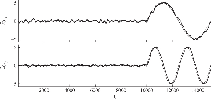
Concatenating the three data sets then produced a combined data set of 15 000 samples. The fault diagnosis scheme introduced in Subsections 8.5.1 and 8.5.2, was now applied to the combined data set for a window size of . Figure 8.11 shows the approximated fault signature each of the data sets. As expected, the estimated fault signature for , and show negligible departures from zero for the first two data sets. For the third data set, an accurate approximation of the squared fault signature and as well as the cross-product term (dashed line) can be seen at first glance.

A closer inspection, however, shows a slight delay with which the original fault signature is approximated, particularly for higher frequency fault signatures in the middle and lower plots in Figure 8.11. According to (8.79), this follows from the moving window approach, which produces an average value for the window. Consequently, for sharply increasing or reducing slopes, like in the case of the sinusoidal signal, the use of the moving window compromises the accuracy of the approximation. The accuracy, however, can be improved by reducing in the window size. This, in turn, has a detrimental effect on the smoothness of the approximation.

The last paragraph in Subsection 8.5.2 raises the question concerning the benefit of the proposed fault diagnosis scheme over a simple moving window average of the process variables. To substantiate the advantage of extracting the squared fault signature from the primary residuals instead of the moving window average of the process variables, Figure 8.12 shows the approximation of the fault signature using a moving window average of the process variables. In order to conduct a fair comparison, the window size for producing the resultant fault signatures in Figure 8.12 was also set to be .

It is interesting to note that the variance of the estimated fault signature for the first two data sets appears to be significantly larger relative to the variance of the estimated fault signature when directly comparing Figures 8.11 and 8.12. In fact, the amplitude of the sinusoidal signals is squared when using the proposed approach compared to the moving window average of the recorded process variables. Secondly, the accuracy of estimating the fault signature in both cases is comparable.

Based on the results of this comparison, the benefit of the proposed fault diagnosis scheme over a simple moving window average of the process variables becomes clear if the amplitude of the sinusoidal is reduced from five to three for example. It can be expected in this case that the variance of the estimated fault signature for the first 10 000 samples increases more substantial relative to the reduced fault signature. This, however, may compromise a clear and distinctive discrimination between the fault signature and normal operating condition, particularly for smaller window sizes.

8.6 Application study of a gearbox system

This section extends the comparison between the non-negative quadratic statistics constructed from the improved residuals with those based on the score variables using an application study of a gearbox system. This system is mounted on an experimental test rig to record normal operating conditions as well as a number of fault conditions.

The next subsection gives a detailed description of the gearbox system and Subsection 8.6.2 explains how the fault condition was injected into the system. Subsection 8.6.3 then summarizes the identification of a PCA-based monitoring model and the construction of improved residuals. Subsection 8.6.4 finally contrasts the performance of the non-negative quadratic statistics based on the improved residuals with those relying on the score variables.

8.6.1 Process description

Given the widespread use of gearbox systems, the performance monitoring of such systems is an important research area in a general engineering context, for example in mechanical and power engineering applications. A gearbox is an arrangement involving a train of gears that transmit power and regulate rotational speed, for example, from an engine to the axle of a car.

Figure 8.13 presents a schematic diagram of the two-stage helical gearbox system (upper plot) and a similar gearbox to that used to generate the recorded vibration data (lower plot). Table 8.5 provides details of the gearbox, which was operated under full-load conditions of 260Nm.

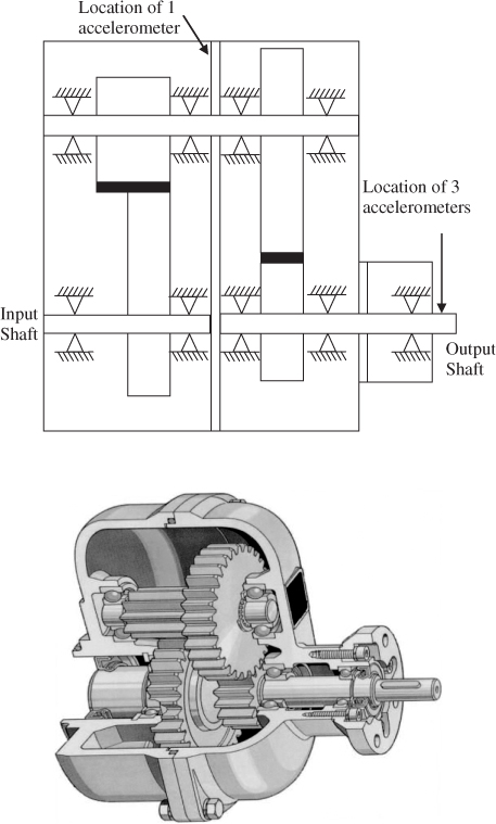
Table 8.5 Specification of gearbox system under study

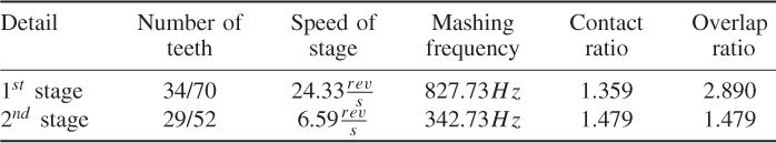
Figure 8.13 shows that a total of four accelerometers are mounted on this gearbox system, which record the vibration signals simultaneously at a frequency of 6.4 kHz. Each recorded data set includes a total of 32 768 samples. Two data sets were recorded that describe a normal operating condition and a further six data sets that represent a gradually increasing fault condition. Figure 8.14 shows the first 5000 samples of each of the four vibration sensors, z₁ to z₄, for one of the reference sets.

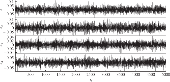
8.6.2 Fault description

For a gearbox system, a tooth breakage is a serious localized fault. Such a fault was simulated here by removing a certain percentage of one tooth in the pinion gear. This tooth removal enabled an experimental representation of a gradual fault advancement under predefined conditions.

The simulated tooth breakage represents the chipping of small parts of one tooth, which is one of the common fault conditions in gearbox systems. For this, the total length of one tooth was gradually removed by increments of 10%. The recorded fault conditions here included a 10% to 50% and a 100% removal of the tooth, that is, a total of six additional data sets that describe the removal of one tooth in various stages. These data sets are referred to here as 10% Fault, 20% Fault to 100% Fault.

Consequences of being unable to detect such faults at early stages include productivity decreases in manufacturing processes, reduced efficiency of engines, equipment damage or even failure. An early detection can provide significant improvements in the reduction of operational and maintenance costs, system down-time, and lead to increased levels of safety, which is an ever-growing concern.

An incipient fault in a mechanical system usually affects certain parameters, such as vibration, noise and temperature. Analyzing these external variables allows the performance monitoring of gears, which are usually inaccessible without dismantling the system. Extracting relevant information from the recorded signals is hence essential for detecting any irregularity that could be caused by tooth breakage or wear.

Baydar and Ball (2001), Baydar et al. (1999, 2001) and Ge et al. (2010) analyzed recorded vibration data from this system using a variety of different methods. Other research work on detecting abnormal operating conditions in gearbox systems include Bartelmus and Zimroz (2009), Hu et al. (2007), Stander et al. (2002), Staszewski and Tomlinson (1997), Tan and Mba (2005), Wang (2008) and Wu et al. (2008).

Since there may be more than one vibration sensor, Baydar and Ball (2001); Baydar et al. (1999, 2001) introduced the application of MSPC to successfully detect tooth defects. In a comprehensive comparison, Baydar et al. (2001) demonstrated that MSPC is equally as sensitive in detecting tooth defects as signal-based approaches but easier to implement in practice. More recent application of MSPC methods in monitoring mechanical systems are given by He et al. (2007, 2009) and Malhi and Gao (2004).

8.6.3 Identification of a monitoring model

This section utilizes PCA to identify a data model according to (2.2). Using one of the reference data sets describing a fault-free operating condition, where no portion of the tooth has been removed, the first steps include the centering and scaling of the data and the estimation of the data correlation matrix.

It follows from Figure 8.14 that the mean value for each vibration signal is close to zero. Estimating the mean yielded values of , , and . The estimated variances for each sensor are , , and .

By inspecting the variances, it is apparent that is five times larger than and also significantly larger than and . Chapter 4 highlighted that significant differences in variance may lead to dominant contributions of process variables with larger variances than the computed score variables.

Jackson (2003) advocated to use of the correlation matrix (i) to ensure that the variables are dimensionless, that is, their dimension for example °C or bar reduces to one and (ii) each process variable has unity variance, which circumvents dominant contributions of variables with large variances. Using the estimated mean and variance, the estimated correlation matrix of the four sensor readings is given by

8.83

The elements of suggest that there is some correlation among sensor readings z₁ and z₂, between variables z₂ and z₄ but variable z₃ shows hardly any correlation with the other sensor readings. Different from the previous application studies in this book, the process variables cannot be seen as highly correlated. Equations (8.84a) and (8.84b) shows the eigendecomposition of

8.84a

8.84b

At first glance, the first two eigenvalues are above one whilst the fourth one is significantly below one and also significantly smaller than the third one. Utilizing the stopping rules for PCA models in Subsection 2.3.1, those that assume a high degree of correlation and a significant contribution of the source signals to the process variables are not applicable here. This, for example, eliminates the VPC and VRE techniques.

An alternative is based on (2.122), which states that the sum of the eigenvalues is equal to the sum of the variances of each process variable. In percentage, the inclusion of n = 1, 2, 3 and 4 latent components yields a variance contribution of 38.66%, 63.91%, 86.45% and 100%, respectively. This suggests the retention of three latent components in the PCA model, as 86% of the variance of the scaled sensor readings can be recovered, and yields the following data model

8.85

Here, , . Estimates of the model and residual subspaces are the first three eigenvectors and the last eigenvector of , respectively. Up to a similarity transformation, , and . Moreover, Ξ and S_ss are assumed to be unknown.

Figure 8.15 compares the estimated distribution function (solid line) with that of a Gaussian distribution of the same mean and variance (dashed-dot line). This comparison shows a good agreement that confirms the validity of the underlying assumptions for the data model in (8.85).

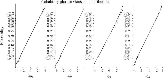
After establishing a PCA model from one of the reference sets, the next step is to determine the window size k₀. To guarantee statistical independence, the performance of a variety of different sizes was tested using the second reference set. This entails the computation of the score variables, based on the PCA model established from the first reference set, the calculation of the four primary and improved residuals and the estimation of the distribution function for each improved residual.

Figure 8.16 contrasts the four estimated distribution functions for the primary residuals and the improved residuals for k₀ = 10, k₀ = 100 and k₀ = 400 with Gaussian ones of the same mean and variance. As expected, very substantial departures from a Gaussian distribution arise for the primary residuals and the improved residuals for k₀ = 10. A closer but still inaccurate approximation emerges for k₀ = 100.

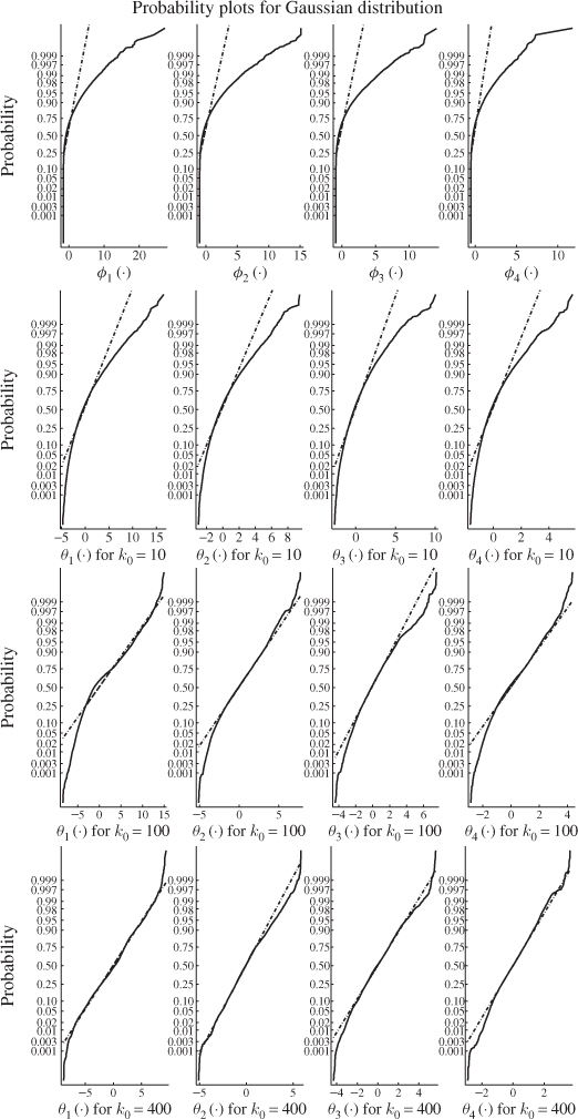
Increasing k₀ to 400 gives rise to a substantially more accurate approximation of a Gaussian distribution. As increasing this number further showed insignificant differences and reducing the number decreased the accuracy, the selection of k₀ = 400 presents a suitable trade-off between accuracy and sensitivity.

8.6.4 Detecting a fault condition

The PCA monitoring model is now applied to each of the recorded data. These include the two reference sets and the six data sets describing the fault condition. The PCA monitoring model determined in the previous subsection allows establishing a total of four non-negative quadratic monitoring statistics:

Given that the correlation matrix and the mean vector of the vibration signals are estimates, the control limits for the Hotelling's T² statistics are obtained by applying (3.5). Applying (3.16) and (3.29) produced the control limits for the Q and Q_θ statistics, respectively. The significance for each control limit is 0.05.

Figure 8.17 shows the performance of the monitoring statistics for each of the eight conditions. As expected, the first two reference conditions did not yield a statistically significant number of violations of the control limit. For the remaining data sets, referring to the removal of 10%, 20%, 30%, 40%, 50% and 100% for one of the tooth in the pinion gear, a different picture emerged. Each of these conditions led to a significant number of violations for each statistic.

Table 8.6 lists the calculated percentage number of violations of each statistic. This analysis confirms that percentages for the two reference conditions are 5% or below, indicating an in-statistical-control behavior of the gearbox system. For each of the fault conditions, however, the percentage number of violations exceeds 5% which hence concludes the performance of the gearbox is out-of-statistical-control.

Table 8.6 Violations of control limits by monitoring statistic in [%].

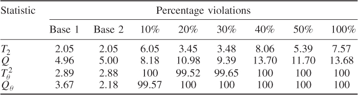
Despite the fact that each monitoring statistic correctly rejected the null hypothesis for each of the fault conditions, it is important to note that the Hotelling's and Q_θ statistic showed a significantly stronger response to the recorded data involving the manipulated pinion gear. This is in line with the observations in Section 8.5 and confirm the sensitivity of the improved residuals in detecting small alterations in the orientation of the model and residual subspaces and the control ellipsoid.

Identifying PCA models on the basis of each of the eight data sets allows to examine the sensitivity issue in more detail. This relies on benchmarking the second reference set and the six data sets describing the fault condition in various stages against the first reference set. More precisely, the departures of the eigenvectors and the differences for each of the four eigenvalues enables assessing the changes in the orientation of the model and residual subspaces and the orientation of the control ellipsoid. These changes can be described as follows

8.86

Here, the indices i = 1, … , 4 and m = 1, … , 7 represent the latent component and the data set, respectively, where m = 1 symbolizes the second reference data set and m = 2, ··· , 7 corresponds to the data sets 10% Fault, 20% Fault, 30% Fault, 40% Fault, 50% Fault and 100% Fault, respectively. Figure 8.18 summarizes the results of applying (8.86). Whilst the eigenvectors and eigenvalues for the correlation matrices of both reference sets are very close to each other, very significant differences can be noticed for data sets 10% Fault to 100% Fault.

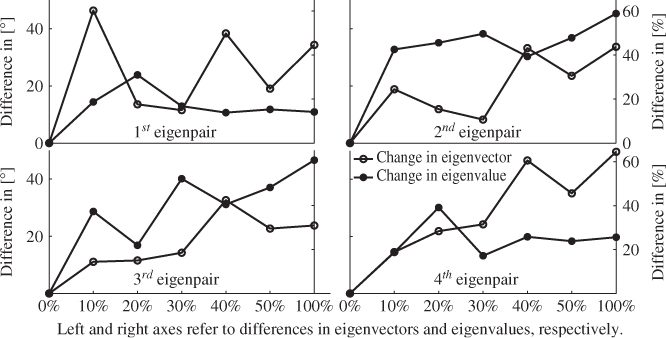
It is interesting to note that the first alteration of the tooth, although only 10% of the length of this tooth was removed, rotated the first eigenvector by around 45°. Apart from the impact of a complete removal of the tooth upon the orientation of the fourth eigenvector, this is the strongest single response.

Similar to the application studies in Subsections 2.1.3 and 6.1.2, the orientation of the model subspace can be assessed by the last eigenvector, which spans the residual subspace. The lower right plot shows a trend that the greater the percentage of the tooth is removed, the larger the rotation of the fourth eigenvector and hence the residual subspace. Given that the model and residual subspaces are complementary subspaces, any rotation of the residual subspace will affect the model subspace too.

With this in mind, it can be concluded that the more severe the fault condition the more significant the impact upon the orientation of the model and residual subspaces. A similar trend, however, cannot be observed for the variance of the fourth eigenvalue. Whilst an initial increase can be noticed, this increase levels off at around 20% if larger portions of the tooth are removed.

Apart from the first eigenpair, the second and third pairs show, approximately, a proportionate response to the severity of the fault condition. The more of the tooth is removed, the larger the variance of the third score variable becomes. The removal of 20% and 30% produce a reduction in the variance of the second score variable, relative to the 10% removal. An increasing trend, however, can also be noticed for the variance of the second score variables with the removal of larger portions.

Based on the experimental data obtained, it can be concluded that the presence of a tooth defect increases the variance of the score variables and with it the variance of the vibration signals, which follows from (2.122). It is interesting to note that the relatively small 10% removal of the tooth has a significantly more pronounced effect on the orientation of the control ellipsoid than the removal of 20% and 30%. It is also interesting to note that the removal of 40% has a similar effect upon the monitoring statistics compared to a complete removal of the tooth.

In contrast, removing 50% of the tooth has a less significant effect on the monitoring model than removing only 40%. As stated above, the only direct relationship between the severity of the fault condition and the impact on the geometry of the monitoring model is the orientation of the residual subspace.

Finally, Table 8.7 summarizes the percentage changes of the variance of the score variables resulting from the fault condition. The score variances are computed with respect to the PCA model established from the first reference set, producing the following percentage changes

8.87

Table 8.7 Changes in variance of score variables

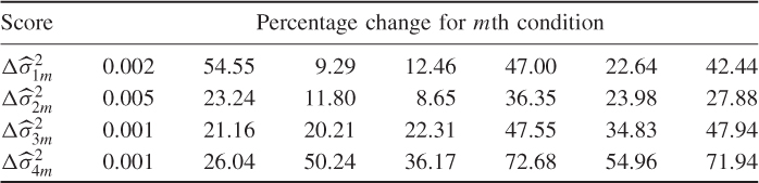
The entries in Table 8.7 confirm the analysis of the individual conditions in Figure 8.18. The most significant impact upon the variance of the first score variable is the 10% removal of the tooth. For the remaining score variables, the most significant effects are the 40% and 100% removal of the tooth. Moreover, the 10% removal has a considerably stronger impact upon the first three score variances than the 20% and 30% removals. The results in Table 8.7 therefore reflect the observations in the upper two plots in Figure 8.17.

8.7 Analysis of primary and improved residuals

As Subsection 8.3.4 gives a detailed analysis of the statistical properties of the primary residuals, this section presents more theoretical aspects of the primary and improved residuals. The section investigates the first and second moments of the primary residuals of the eigenvectors , after presenting a detailed proof of the CLT for a sum of random variables that are i.i.d. This is followed by an examination of the covariance matrices for ϕ_i and to fault conditions. Finally, Subsection 8.7.3 outlines and proves that the non-negative quadratic statistics obtained from the improved residuals are more sensitive than those computed from the score variables.

8.7.1 Central limit theorem

According to (8.16), the statistical local approach relies on a vector-valued function of improved residuals which are, theoretically, an infinite sum of primary residuals. This subsection shows that

8.88

converges in distribution to when K → ∞. To simplify the analysis here, we examine the jth element of , ϕ_j. The definition of the primary residuals in the preceding sections outlined that they have a mean of zero, so we can safely assume here that E{ϕ_j} = 0. Moreover, for the variance of ϕ_j, , we write . In summary, the first and second moments of ϕ_j are

8.89

With this in mind, the jth element in (8.88) can be reformulated as follows

8.90

Given that the samples, z₀(k), are drawn independently from the distribution function , the instances of the primary residuals ϕ_j(k) are also drawn independently from the distribution function F(ϕ_j) in (8.55). Moreover, as pointed out before, each instance is drawn from the same distribution function F(ϕ_j) and each of these instances are i.i.d. With respect to the preceding discussion, we can now formulate a simplified version of the Lindeberg-Lévy theorem, defining the CLT for the infinite i.i.d. sequence of ϕ_j.

 

The first step is to substitute the definition of θ_j into (8.91). With respect to the definition of the characteristic function, this gives rise to

8.92

The fact that the random variables ϕ_j(1), ϕ_j(2), …  , ϕ_j(K) are i.i.d. implies that their distribution and characteristic functions are identical. The product in (8.92) can therefore be simplified to

8.93

Here, , that is, the characteristic function of ϕ_j is the Kth root of the characteristic function of θ_j. The next step is to develop a Taylor series of for c = 0

8.94

where the last term, , , is the Lagrangian remainder. The relationships can be obtained from the definition of the characteristic function

8.95

According to Equation (8.89), the relationships up to order three are therefore:

• ;
• ;
• 
• 

Here, is a small correction term and is the third moment of ϕ_j. Substituting these relationships in (8.94) yields

8.96

Substituting (8.96) into (8.93) gives rise to

8.97

Note that the characteristic function of the standard Gaussian distribution function is and that . Therefore, the expression in (8.97) asymptotically converges to

8.98

This follows from .

8.7.2 Further statistical properties of primary residuals

After proving the CLT, we now focus on discussing further properties of the primary residuals. Subsection 8.3.4 shows the first two moments for the primary residuals . This subsection determines the covariance and cross-covariance matrices for the primary residuals t_iz₀ − λ_ip_i. It also discusses how the covariance matrices of and t_iz₀ − λ_ip_i are affected by a change in the eigenvalues and eigenvectors.

8.7.2.1 Covariance matrices of primary residuals in equation (8.20)

The determination of the covariance and cross-covariance matrices for the primary residual vectors , and and , i ≠ j, requires the substitution of and into and , respectively.

Covariance matrix

Starting with the covariance matrix

8.99

the expectation on the right hand side of (8.99) can be analyzed separately by substituting , which yields

8.100a

8.100b

8.100c

The above simplifications follow from E{t_it_j} = 0 for all i ≠ j. The fact that there are terms in (8.100a) gives rise to the following separation.

• For i ≠ j ≠ m, there are a total of terms in this case, which produces

• There are n_z − 1 cases of i ≠ j = m, which yield the general expression

• The remaining term, i = j = m, is equal to

Putting this all together, (8.100a) reduces to

8.101

Substituting (8.100a) to (8.101) into (8.99) finally yields

8.102

Cross-covariance matrix

The matrix , i ≠ j and i, j = 1, 2, … , n_z, is similar to that in (8.99) and is given by

8.103

Using the simplifications applied to (8.99), (8.103) reduces to

8.104a

8.104b

8.104c

Given that E{t_it_jt_mt_m} = 0 for all m ≠ i, m ≠ j and m ≠ j, m ≠ i, (8.104a) reduces to

8.105

Putting it all together, (8.103) finally yields

8.106

8.7.2.2 Covariance matrix for a change in λ_i

Under the assumption that the eigenvectors remain constant, changing the covariance of the ith score variable to be λ_i + Δλ_i results in the following alteration of

8.107

The expectation of is

8.108

which implies that the covariance matrix matrix becomes

8.109

Thus, a change in the eigenvalues yield the same covariance matrix for and .

8.7.2.3 Covariance matrix for change in p_i

An alteration of the eigenvector, , does not have the same isolated impact upon , as is the case for a change in the eigenvalue. This is because a rotation of ith eigenvector affects more then just this eigenvector, since the eigenvectors are mutually orthonormal. If we restrict this examination by assuming that only the ith eigenvector is altered and the remaining n_z − 1 eigenvectors and the score covariance matrix remain unchanged, becomes

8.110

Note that for all j ≠ i. The expectation of is

8.111

which gives rise to the following covariance matrix

8.112

The difference between the covariance matrices of and is therefore

8.113

8.7.2.4 Covariance of for a change in λ_i

8.114

and has the following expectation

8.115

which gives rise to the following covariance

8.116

which follows from (8.48). The difference between and is therefore

8.117

8.7.2.5 Covariance of for a change in p_i

Changing p_i to p_i + Δp_i implies that it is no longer orthogonal to all of the remaining n_z − 1 eigenvectors. Assuming that ||p_i + Δp_i|| = 1 and defining the n_z loading vectors by , for all j ≠ i, the expectation of becomes

8.118

Next, substituting into (8.118) gives rise to

8.119

That is interesting and follows from the assumption that the length of ||p₁|| = ||p_i + Δp_i|| = 1, that is, . Using the mean value , the covariance of is equal to

8.120

It follows that , since .

8.7.3 Sensitivity of statistics based on improved residuals

The previous sections showed that the primary residuals are sufficient for detecting changes in the underlying geometry of the data model in (2.2). Furthermore, the mean and variance of these residuals is 0 and , respectively, and there is no covariance between the ith and jth primary residuals, that is, .

Furthermore, the primary residuals are i.i.d. implying that the improved residuals are asymptotically Gaussian distributed and have the same mean, variance and covariance as the primary residuals. The covariance matrix for the vector containing the improved residuals of the first n eigenpairs of is equal to , where is the diagonal matrix storing the n dominant eigenvalues of .

The sensitivity in detecting various fault conditions is now examined for a simple sensor or actuator bias. The scope of Project 3 in the tutorial section covers more complex process faults that alter the eigenvectors and eigenvalues by contrasting the sensitivity of the non-negative quadratic statistics constructed from the improved residuals with those based on the score variables.

8.7.3.1 Sensitivity for detecting sensor or actuator bias

The data model describing a sensor fault is as follows

8.121

According to Table 2.1, the effect of a sensor or actuator fault can be described by an offset term or a bias and a stochastic term or a precision degradation. Besides bias and precision degradation, both terms can also describe a complete failure or a drift if the offset term is assumed to be time varying and deterministic. For a sensor bias, described by a constant bias term Δz₀, the ith improved residual becomes

8.122

Expectation of

The expectation follows from

8.123

Variance of

Defining the mean-centered by

8.124

simplifies the determination of the variance of

8.125

which yields that . The next step is to examine the impact of Δz₀ upon the non-negative quadratic monitoring statistics.

Effect of Δz₀ upon

This impact can be described by

8.126

which requires examining

8.127

from which it follows that

8.128

Equation (8.126) can now be evaluated, which yields

8.129

This compares favorably to the sensitivity of the conventional Hotelling's T² statistic

8.130

The difference between (8.128) and (8.129) is then a measure for sensitivity of the Hotelling's T² statistic constructed from the improved residuals and the score variables

8.131

For the Hotelling's T² statistics, (8.131) outlines that, irrespective of the window length k₀, the non-negative quadratic statistics constructed from the improved residuals is more sensitive to a set of sensor or actuator biases. Moreover, this equation also highlights that the larger the value of k₀ the more significant this increase in sensitivity becomes.

Constructing the residual Q statistics on the basis of (3.19) yields the same conclusion. Under the assumption that , the n_z − n required eigenvalues for constructing the and , . Since , (8.131) also confirms that the increase in sensitivity is more pronounced for the Q statistic.

The application studies in Sections 8.4 and 8.6 confirm the above findings. More precisely, Figures 8.7, 8.9 and 8.17 illustrate that the non-negative quadratic statistics based on the score variables show sporadic violations of their control limits which, however, exceeded the significance level. In contrast, the statistics constructed from the improved residuals showed a considerably stronger response and produced, in almost each case, a constant violation of their control limits.

8.8 Tutorial session

Question 1:

Describe under which conditions conventional scatter diagrams, the Hotelling's T² statistic and the Q statistic are insensitive to fault conditions. What is the effect of such changes upon Type II errors?

Question 2:

Referring to Question 1, analyze how these changes can be detected.

Question 3:

Explain why the primary residuals are difficult to use for constructing monitoring charts. How can the associated problems be overcome?

Question 4:

What is the problem of using primary residuals that are based on the eigenvectors of the data covariance matrix? Are the primary residuals related to the eigenvalues of the data covariance matrix also affected by this problem? Are both types of primary residuals sensitive to geometric changes in the model and residual subspaces as well as changes in the variances of the source and error variables?

Question 5:

Describe the properties of the primary and improved residuals based on the eigenvalues of the covariance matrix.

Question 6:

Discuss the assumptions under which the central limit theorem holds true. What are the conditions under which the central limit theorem does not hold true?

Project 1:

Use a Monte Carlo simulation based on the second intuitive example, described in (8.8), augment the stochastic vector z₀ by a time-varying mean vector and comment on the Type I and II errors. For PCA, discuss how to develop an adaptive monitoring approach to construct primary residuals. How can such an adaptive approach be utilized to determine improved residuals?

Project 2:

Develop primary and improved residuals on the basis of the PLS objective functions for determining the weight and loading vectors. Can a fault that (i) only affects the input variables, or (ii) only affects the output variables, or (iii) affects the input and the output variables, be detected? Discuss the results and propose a reliable monitoring scheme for detecting geometric changes in the weight and loading vectors and the variance of the score variables.

Project 3:

Assume that a fault condition affects the ith eigenvector and/or eigenvalue of the covariance matrix . Similar to the analysis in Subsection 8.7.3, develop and contrast the relationships describing the impact of such a change upon the Hotelling's T² and statistics.

 

 

¹ This relatively large range outlines, again, the problem of selecting an appropriate size for the reference data set, discussed in Section 6.4 and Subsection 7.3.6.

² !! is the double factorial and the product of the odd numbers only, e.g. 9!! = 1 · 3 · 5 · 7 · 9 = 945.