
8 Process and Measurement System Capability Analysis
CHAPTER OUTLINE
8.2 PROCESS CAPABILITY ANALYSIS USING A HISTOGRAM OR A PROBABILITY PLOT
8.3.1 Use and Interpretation of Cp
8.3.2 Process Capability Ratio for an Off-Center Process
8.3.3 Normality and the Process Capability Ratio
8.3.4 More about Process Centering
8.3.5 Confidence Intervals and Tests on Process Capability Ratios
8.4 PROCESS CAPABILITY ANALYSIS USING A CONTROL CHART
8.5 PROCESS CAPABILITY ANALYSIS USING DESIGNED EXPERIMENTS
8.6 PROCESS CAPABILITY ANALYSIS WITH ATTRIBUTE DATA
8.7 GAUGE AND MEASUREMENT SYSTEM CAPABILITY STUDIES
8.7.1 Basic Concepts of Gauge Capability
8.7.2 The Analysis of Variance Method
8.7.3 Confidence Intervals in Gauge R & R Studies
8.7.4 False Defectives and Passed Defectives
8.7.5 Attribute Gauge Capability
8.7.6 Comparing Customer and Supplier Measurement Systems
8.8 SETTING SPECIFICATION LIMITS ON DISCRETE COMPONENTS
8.9 ESTIMATING THE NATURAL TOLERANCE LIMITS OF A PROCESS
8.9.1 Tolerance Limits Based on the Normal Distribution
8.9.2 Nonparametric Tolerance Limits
Supplemental Material for Chapter 8
S8.1 Fixed Versus Random Factors in the Analysis of Variance
S8.2 More About Analysis of Variance Methods for Measurement Systems Capability Studies
The supplemental material is on the textbook Website www.wiley.com/college/montgomery.
CHAPTER OVERVIEW AND LEARNING OBJECTIVES
In Chapter 6, we formally introduced the concept of process capability, or how the inherent variability in a process compares with the specifications or requirements for the product. Process capability analysis is an important tool in the DMAIC process, with application in both the Analyze and Improve steps. This chapter provides more extensive discussion of process capability, including several ways to study or analyze the capability of a process. We believe that the control chart is a simple and effective process capability analysis technique. We also extend the presentation of process capability ratios that we began in Chapter 6, showing how to interpret these ratios and discussing their potential dangers. The chapter also contains information on evaluating measurement system performance, illustrating graphical methods, as well as techniques based on the analysis of variance. Measurement systems analysis is used extensively in DMAIC, principally during the Measure step. We also discuss setting specifications on individual discrete parts or components and estimating the natural tolerance limits of a process.
After careful study of this chapter, you should be able to do the following:
1. Investigate and analyze process capability using control charts, histograms, and probability plots
2. Understand the difference between process capability and process potential
3. Calculate and properly interpret process capability ratios
4. Understand the role of the normal distribution in interpreting most process capability ratios
5. Calculate confidence intervals on process capability ratios
6. Conduct and analyze a measurement systems capability (or gauge R & R) experiment
7. Estimate the components of variability in a measurement system
8. Set specifications on components in a system involving interaction components to ensure that overall system requirements are met
9. Estimate the natural limits of a process from a sample of data from that process
8.1 Introduction
Statistical techniques can be helpful throughout the product cycle, including development activities prior to manufacturing, in quantifying process variability, in analyzing this variability relative to product requirements or specifications, and in assisting development and manufacturing in eliminating or greatly reducing this variability. This general activity is called process capability analysis.
Process capability refers to the uniformity of the process. Obviously, the variability of critical-to-quality characteristics in the process is a measure of the uniformity of output. There are two ways to think of this variability:
1. The natural or inherent variability in a critical-to-quality characteristic at a specified time—that is, “instantaneous” variability
2. The variability in a critical-to-quality characteristic over time
We present methods for investigating and assessing both aspects of process capability. Determining process capability is an important part of the DMAIC process. It is used primarily in the Analyze step, but it also can be useful in other steps, such as Improve.

![]() FIGURE 8.1 Upper and lower natural tolerance limits in the normal distribution.
FIGURE 8.1 Upper and lower natural tolerance limits in the normal distribution.
It is customary to take the Six Sigma spread in the distribution of the product quality characteristic as a measure of process capability. Figure 8.1 shows a process for which the quality characteristic has a normal distribution with mean μ and standard deviation σ. The upper and lower natural tolerance limits of the process fall at μ + 3σ and μ – 3σ, respectively—that is,
UNTL = μ + 3σ
LNTL = μ – 3σ
For a normal distribution, the natural tolerance limits include 99.73% of the variable, or put another way, only 0.27% of the process output will fall outside the natural tolerance limits. Two points should be remembered:
1. 0.27% outside the natural tolerances sounds small, but this corresponds to 2,700 non-conforming parts per million.
2. If the distribution of process output is non-normal, then the percentage of output falling outside μ ± 3σ may differ considerably from 0.27%.
We define process capability analysis as a formal study to estimate process capability. The estimate of process capability may be in the form of a probability distribution having a specified shape, center (mean), and spread (standard deviation). For example, we may determine that the process output is normally distributed with mean μ = 1.0 cm and standard deviation σ = 0.001 cm. In this sense, a process capability analysis may be performed without regard to specifications on the quality characteristic. Alternatively, we may express process capability as a percentage outside of specifications. However, specifications are not necessary to process capability analysis.
A process capability study usually measures functional parameters or critical-to-quality characteristics on the product, not the process itself. When the analyst can directly observe the process and can control or monitor the data-collection activity, the study is a true process capability study, because by controlling the data collection and knowing the time sequence of the data, inferences can be made about the stability of the process over time. However, when we have available only sample units of product, perhaps obtained from the supplier, and there is no direct observation of the process or time history of production, then the study is more properly called product characterization. In a product characterization study we can only estimate the distribution of the product quality characteristic or the process yield (fraction conforming to specifications); we can say nothing about the dynamic behavior of the process or its state of statistical control. In order to make a reliable estimate of process capability, the process must be in statistical control. Otherwise, the predictive inference about process performance can be seriously in error. Data collected at different time periods could lead to different conclusions.
Process capability analysis is a vital part of an overall quality-improvement program. Among the major uses of data from a process capability analysis are the following:
1. Predicting how well the process will hold the tolerances
2. Assisting product developers/designers in selecting or modifying a process
3. Assisting in establishing an interval between sampling for process monitoring
4. Specifying performance requirements for new equipment
5. Selecting between competing suppliers and other aspects of supply chain management
6. Planning the sequence of production processes when there is an interactive effect of processes on tolerances
7. Reducing the variability in a process
Thus, process capability analysis is a technique that has application in many segments of the product cycle, including product and process design, supply chain management, production or manufacturing planning, and manufacturing.
Three primary techniques are used in process capability analysis: histograms or probability plots, control charts, and designed experiments. We will discuss and illustrate each of these methods in the next three sections. We will also discuss the process capability ratio (PCR) introduced in Chapter 6 and some useful variations of this ratio.
8.2 Process Capability Analysis Using a Histogram or a Probability Plot
8.2.1 Using the Histogram
The histogram can be helpful in estimating process capability. Alternatively, a stem-and-leaf plot may be substituted for the histogram. At least 100 or more observations should be available for the histogram (or the stem-and-leaf plot) to be moderately stable so that a reasonably reliable estimate of process capability may be obtained. If the quality engineer has access to the process and can control the data-collection effort, the following steps should be followed prior to data collection:
1. Choose the machine or machines to be used. If the results based on one (or a few) machines are to be extended to a larger population of machines, the machine selected should be representative of those in the population. Furthermore, if the machine has multiple workstations or heads, it may be important to collect the data so that head-to-head variability can be isolated. This may imply that designed experiments should be used.
2. Select the process operating conditions. Carefully define conditions, such as cutting speeds, feed rates, and temperatures, for future reference. It may be important to study the effects of varying these factors on process capability.
3. Select a representative operator. In some studies, it may be important to estimate operator variability. In these cases, the operators should be selected at random from the population of operators.
4. Carefully monitor the data-collection process, and record the time order in which each unit is produced.
The histogram, along with the sample average ![]() and sample standard deviation s, provides information about process capability. You may wish to review the guidelines for constructing histograms in Chapter 3.
and sample standard deviation s, provides information about process capability. You may wish to review the guidelines for constructing histograms in Chapter 3.
EXAMPLE 8.1 Estimating Process Capability with a Histogram
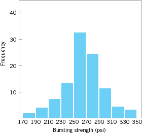
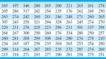
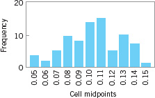
Figure 8.2 presents a histogram of the bursting strength of 100 glass containers. The data are shown in Table 8.1. What is the capability of the process?
SOLUTION
Analysis of the 100 observations gives
![]()
Consequently, the process capability would be estimated as
![]()
or
![]()
![]() FIGURE 8.2 Histogram for the bursting-strength data.
FIGURE 8.2 Histogram for the bursting-strength data.
Furthermore, the shape of the histogram implies that the distribution of bursting strength is approximately normal. Thus, we can estimate that approximately 99.73% of the bottles manufactured by this process will burst between 168 and 360 psi. Note that we can estimate process capability independently of the specifications on bursting strength.
![]() TABLE 8.1
TABLE 8.1
Bursting Strengths for 100 Glass Containers
An advantage of using the histogram to estimate process capability is that it gives an immediate, visual impression of process performance. It may also immediately show the reason for poor process performance. For example, Figure 8.3a shows a process with adequate potential capability, but the process target is poorly located, whereas Figure 8.3b shows a process with poor capability resulting from excess variability. Histograms do not provide any information about the state of statistical control of the process. So conclusions about capability based on the histogram depend on the assumption that the process is in control.

![]() FIGURE 8.3 Some reasons for poor process capability. (a) Poor process centering. (b) Excess process variability.
FIGURE 8.3 Some reasons for poor process capability. (a) Poor process centering. (b) Excess process variability.
8.2.2 Probability Plotting
Probability plotting is an alternative to the histogram that can be used to determine the shape, center, and spread of the distribution. It has the advantage that it is unnecessary to divide the range of the variable into class intervals, and it often produces reasonable results for moderately small samples (which the histogram will not). Generally, a probability plot is a graph of the ranked data versus the sample cumulative frequency on special paper with a vertical scale chosen so that the cumulative distribution of the assumed type is a straight line. In Chapter 3 we discussed and illustrated normal probability plots. These plots are very useful in process capability studies.
To illustrate the use of a normal probability plot in a process capability study, consider the following 20 observations on glass container bursting strength: 197, 200, 215, 221, 231, 242, 245, 258, 265, 265, 271, 275, 277, 278, 280, 283, 290, 301, 318, and 346. Figure 8.4 is the normal probability plot of strength. Note that the data lie nearly along a straight line, implying that the distribution of bursting strength is normal. Recall from Chapter 4 that the mean of the normal distribution is the 50th percentile, which we may estimate from Figure 8.4 as approximately 265 psi, and the standard deviation of the distribution is the slope of the straight line. It is convenient to estimate the standard deviation as the difference between the 84th and the 50th percentiles. For the strength data shown above and using Figure 8.4, we find that
![]()
Note that ![]() and
and ![]() are not far from the sample average
are not far from the sample average ![]() and standard deviation s = 32.02.
and standard deviation s = 32.02.
The normal probability plot can also be used to estimate process yields and fallouts. For example, the specification on container strength is LSL = 200 psi. From Figure 8.4, we would estimate that about 5% of the containers manufactured by this process would burst below this limit. Since the probability plot provides no information about the state of statistical control of the process, care should be taken in drawing these conclusions. If the process is not in control, these estimates may not be reliable.
Care should be exercised in using probability plots. If the data do not come from the assumed distribution, inferences about process capability drawn from the plot may be seriously in error. Figure 8.5 presents a normal probability plot of times to failure (in hours) of a valve in a chemical plant. From examining this plot, we can see that the distribution of failure time is not normal.
An obvious disadvantage of probability plotting is that it is not an objective procedure. It is possible for two analysts to arrive at different conclusions using the same data. For this reason, it is often desirable to supplement probability plots with more formal statistically based goodness-of-fit tests. A good introduction to these tests is in Shapiro (1980). Augmenting the interpretation of a normal probability plot with the Shapiro–Wilk test for normality can make the procedure much more powerful and objective.

![]() FIGURE 8.4 Normal probability plot of the container-strength data.
FIGURE 8.4 Normal probability plot of the container-strength data.

![]() FIGURE 8.5 Normal probability plot of time to failure of a valve.
FIGURE 8.5 Normal probability plot of time to failure of a valve.
![]() FIGURE 8.6 Regions in the β1, β2 plane for various distributions. (From Statistical Models in Engineering by G. J. Hahn and S. S. Shapiro, John Wiley: New York, 1967.)
FIGURE 8.6 Regions in the β1, β2 plane for various distributions. (From Statistical Models in Engineering by G. J. Hahn and S. S. Shapiro, John Wiley: New York, 1967.)
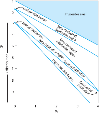
Choosing the distribution to fit the data is also an important step in probability plotting. Sometimes we can use our knowledge of the physical phenomena or past experience to suggest the choice of distribution. In other situations, the display in Figure 8.6 may be useful in selecting a distribution that describes the data. This figure shows the regions in the β1, β2 plane for several standard probability distributions, where β1 and β2 are the measures of skewness and kurtosis, respectively. To use Figure 8.6, calculate estimates of skewness and kurtosis from the sample—say,
and
where
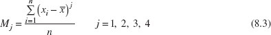
and plot the point (![]() ) on the graph. If the plotted point falls close to a point, line, or region that corresponds to one of the distributions in the figure, then this distribution is a logical choice to use as a model for the data. If the point falls in regions of the β1, β2 plane where none of the distributions seems appropriate, other, more general probability distributions, such as the Johnson or Pearson families of distributions, may be required. A note of caution should be sounded here: The skewness and kurtosis statistics are not reliable unless they are computed from very large samples. Procedures similar to that in Figure 8.6 for fitting these distributions and graphs are in Hahn and Shapiro (1967).
) on the graph. If the plotted point falls close to a point, line, or region that corresponds to one of the distributions in the figure, then this distribution is a logical choice to use as a model for the data. If the point falls in regions of the β1, β2 plane where none of the distributions seems appropriate, other, more general probability distributions, such as the Johnson or Pearson families of distributions, may be required. A note of caution should be sounded here: The skewness and kurtosis statistics are not reliable unless they are computed from very large samples. Procedures similar to that in Figure 8.6 for fitting these distributions and graphs are in Hahn and Shapiro (1967).
8.3 Process Capability Ratios
8.3.1 Use and Interpretation of Cp
It is frequently convenient to have a simple, quantitative way to express process capability. One way to do so is through the process capability ratio (PCR) Cp first introduced in Chapter 6. Recall that

where USL and LSL are the upper and lower specification limits, respectively. Cp and other process capability ratios are used extensively in industry. They are also widely misused. We will point out some of the more common abuses of process capability ratios. An excellent recent book on process capability ratios that is highly recommended is Kotz and Lovelace (1998). There is also extensive technical literature on process capability analysis and process capability ratios. The review paper by Kotz and Johnson (2002) and the bibliography (papers) by Spiring, Leong, Cheng, and Yeung (2003) and Yum and Kim (2011) are excellent sources.
In a practical application, the process standard deviation σ is almost always unknown and must be replaced by an estimate σ. To estimate σ we typically use either the sample standard deviation s or ![]() (when variables control charts are used in the capability study). This results in an estimate of Cp—say,
(when variables control charts are used in the capability study). This results in an estimate of Cp—say,

To illustrate the calculation of Cp, recall the semiconductor hard-bake process first analyzed in Example 6.1 using ![]() and R charts. The specifications on flow width are USL = 1.00 microns and LSL = 2.00 microns, and from the R chart we estimated
and R charts. The specifications on flow width are USL = 1.00 microns and LSL = 2.00 microns, and from the R chart we estimated ![]() . Thus, our estimate of the PCR Cp is
. Thus, our estimate of the PCR Cp is
![]()
In Chapter 6, we assumed that flow width is approximately normally distributed (a reasonable assumption, based on the histogram in Fig. 8.7) and the cumulative normal distribution table in the Appendix was used to estimate that the process produces approximately 350 ppm (parts per million) defective. Please note that this conclusion depends on the assumption that the process is in statistical control.
The PCR Cp in equation 8.4 has a useful practical interpretation—namely,

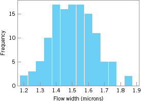
![]() FIGURE 8.7 Histogram of flow width from Example 6.1.
FIGURE 8.7 Histogram of flow width from Example 6.1.
is the percentage of the specification band used up by the process. The hard-bake process uses
![]()
percent of the specification band.
Equations 8.4 and 8.5 assume that the process has both upper and lower specification limits. For one-sided specifications, one-sided process-capability ratios are used. One-sided PCRs are defined as follows.

Estimates ![]() and
and ![]() would be obtained by replacing μ and σ in equations 8.7 and 8.8 by estimates
would be obtained by replacing μ and σ in equations 8.7 and 8.8 by estimates ![]() and
and ![]() , respectively.
, respectively.
EXAMPLE 8.2 One-Sided Process-Capability Ratios
Construct a one-sided process-capability ratio for the container bursting-strength data in Example 8.1. Suppose that the lower specification limit on bursting strength is 200 psi.
SOLUTION
We will use ![]() and s = 32 as estimates of μ and σ, respectively, and the resulting estimate of the one-sided lower process-capability ratio is
and s = 32 as estimates of μ and σ, respectively, and the resulting estimate of the one-sided lower process-capability ratio is
![]()
The fraction of defective containers produced by this process is estimated by finding the area to the left of Z = (LSL – μ)/σ = (200 – 264)/32 = −2 under the standard normal distribution. The estimated fallout is about 2.28% defective, or about 22,800 nonconforming containers per million. Note that if the normal distribution were an inappropriate model for strength, then this last calculation would have to be performed using the appropriate probability distribution. This calculation also assumes an in-control process.
![]() TABLE 8.2
TABLE 8.2
Values of the Process Capability Ratio (Cp) and Associated Process Fallout for a Normally Distributed Process (in Defective ppm) That Is in Statistical Control
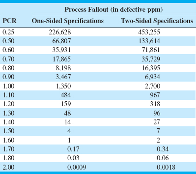
The process capability ratio is a measure of the ability of the process to manufacture product that meets the specifications. Table 8.2 presents several values of the PCR Cp along with the associated values of process fallout, expressed in defective parts or nonconforming units of product per million (ppm). To illustrate the use of Table 8.2, notice that a PCR for a normally distributed stable process of Cp = 1.00 implies a fallout rate of 2,700 ppm for two-sided specifications, whereas a PCR of Cp = 1.50 for this process implies a fallout rate of 4 ppm for one-sided specifications.
The ppm quantities in Table 8.2 were calculated using the following important assumptions:
1. The quality characteristic has a normal distribution.
2. The process is in statistical control.
3. In the case of two-sided specifications, the process mean is centered between the lower and upper specification limits.
These assumptions are absolutely critical to the accuracy and validity of the reported numbers, and if they are not valid, then the reported quantities may be seriously in error. For example, Somerville and Montgomery (1996) report an extensive investigation of the errors in using the normality assumption to make inferences about the ppm level of a process when in fact the underlying distribution is non-normal. They investigated various non-normal distributions and observed that errors of several orders of magnitude can result in predicting ppm by erroneously making the normality assumption. Even when using a t distribution with as many as 30 degrees of freedom, substantial errors result. Thus even though a t distribution with 30 degrees of freedom is symmetrical and almost visually indistinguishable from the normal, the longer and heavier tails of the t distribution make a significant difference when estimating the ppm. Consequently, symmetry in the distribution of process output alone is insufficient to ensure that any PCR will provide a reliable prediction of process ppm. We will discuss the non-normality issue in more detail in Section 8.3.3.
![]() TABLE 8.3
TABLE 8.3
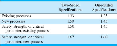
Recommended Minimum Values of the Process Capability Ratio
Stability or statistical control of the process is also essential to the correct interpretation of any PCR. Unfortunately, it is fairly common practice to compute a PCR from a sample of historical process data without any consideration of whether or not the process is in statistical control. If the process is not in control, then of course its parameters are unstable, and the value of these parameters in the future is uncertain. Thus the predictive aspects of the PCR regarding process ppm performance are lost.
Finally, remember that what we actually observe in practice is an estimate of the PCR. This estimate is subject to error in estimation, since it depends on sample statistics. English and Taylor (1993) report that large errors in estimating PCRs from sample data can occur, so the estimate one actually has at hand may not be very reliable. It is always a good idea to report the estimate of any PCR in terms of a confidence interval. We will show how to do this for some of the commonly used PCRs in Section 8.3.5.
Table 8.3 presents some recommended guidelines for minimum values of the PCR. The bottle-strength characteristic is a parameter closely related to the safety of the product; bottles with inadequate pressure strength may fail and injure consumers. This implies that the PCR should be at least 1.45. Perhaps one way the PCR could be improved would be by increasing the mean strength of the containers—say, by pouring more glass in the mold.
We point out that the values in Table 8.3 are only minimums. In recent years, many companies have adopted criteria for evaluating their processes that include process capability objectives that are more stringent than those of Table 8.3. For example, a Six Sigma company would require that when the process mean is in control, it will not be closer than six standard deviations from the nearest specification limit. This, in effect, requires that the minimum acceptable value of the process capability ratio will be at least 2.0.
8.3.2 Process Capability Ratio for an Off-Center Process
The process capability ratio Cp does not take into account where the process mean is located relative to the specifications. Cp simply measures the spread of the specifications relative to the Six Sigma spread in the process. For example, the top two normal distributions in Figure 8.8 both have Cp = 2.0, but the process in panel (b) of the figure clearly has lower capability than the process in panel (a) because it is not operating at the midpoint of the interval between the specifications.
This situation may be more accurately reflected by defining a new process capability ratio (PCR)—Cpk—that takes process centering into account. This quantity is

Note that Cpk is simply the one-sided PCR for the specification limit nearest to the process average. For the process shown in Figure 8.8b, we would have

Generally, if Cp = Cpk, the process is centered at the midpoint of the specifications, and when Cpk < Cp the process is off center.
The magnitude of Cpk relative to Cp is a direct measure of how off center the process is operating. Several commonly encountered cases are illustrated in Figure 8.8. Note in panel (c) of Figure 8.8 that Cpk = 1.0 while Cp = 2.0. One can use Table 8.2 to get a quick estimate of potential improvement that would be possible by centering the process. If we take Cp = 1.0 in Table 8.2 and read the fallout from the one-sided specifications column, we can estimate the actual fallout as 1,350 ppm. However, if we can center the process, then Cp = 2.0 can be achieved, and Table 8.2 (using Cp = 2.0 and two-sided specifications) suggests that the potential fallout is 0.0018 ppm, an improvement of several orders of magnitude in process performance. Thus, we usually say that Cp measures potential capability in the process, whereas Cpk measures actual capability.

![]() FIGURE 8.8 Relationship of Cp and Cpk.
FIGURE 8.8 Relationship of Cp and Cpk.
Panel (d) of Figure 8.8 illustrates the case in which the process mean is exactly equal to one of the specification limits, leading to Cpk = 0. As panel (e) illustrates, when Cpk < 0 the implication is that the process mean lies outside the specifications. Clearly, if Cpk < −1, the entire process lies outside the specification limits. Some authors define Cpk to be nonnegative, so that values less than zero are defined as zero.
Many quality-engineering authorities have advised against the routine use of process capability ratios such as Cp and Cpk (or the others discussed later in this section) on the grounds that they are an oversimplification of a complex phenomenon. Certainly, any statistic that combines information about both location (the mean and process centering) and variability and that requires the assumption of normality for its meaningful interpretation is likely to be misused (or abused). Furthermore, as we will see, point estimates of process capability ratios are virtually useless if they are computed from small samples. Clearly, these ratios need to be used and interpreted very carefully.
8.3.3 Normality and the Process Capability Ratio
An important assumption underlying our discussion of process capability and the ratios Cp and Cpk is that their usual interpretation is based on a normal distribution of process output. If the underlying distribution is non-normal, then as we previously cautioned, the statements about expected process fallout attributed to a particular value of Cp or Cpk may be in error.
To illustrate this point, consider the data in Figure 8.9, which is a histogram of 80 measurements of surface roughness on a machined part (measured in microinches). The upper specification limit is at USL = 32 microinches. The sample average and standard deviation are ![]() = 10.44 and S = 3.053, implying that
= 10.44 and S = 3.053, implying that ![]() , and Table 8.2 would suggest that the fallout is less than one part per billion. However, since the histogram is highly skewed, we are fairly certain that the distribution is non-normal. Thus, this estimate of capability is unlikely to be correct.
, and Table 8.2 would suggest that the fallout is less than one part per billion. However, since the histogram is highly skewed, we are fairly certain that the distribution is non-normal. Thus, this estimate of capability is unlikely to be correct.
One approach to dealing with this situation is to transform the data so that in the new, transformed metric the data have a normal distribution appearance. There are various graphical and analytical approaches to selecting a transformation. In this example, a reciprocal transformation was used. Figure 8.10 presents a histogram of the reciprocal values x* = 1/x. In the transformed scale, ![]() * = .01025 and s* = 0.0244, and the original upper specification limit becomes 1/32 = 0.03125. This results in a value of
* = .01025 and s* = 0.0244, and the original upper specification limit becomes 1/32 = 0.03125. This results in a value of ![]() , which implies that about 1,350 ppm are outside of specifications. This estimate of process performance is clearly much more realistic than the one resulting from the usual “normal theory” assumption.
, which implies that about 1,350 ppm are outside of specifications. This estimate of process performance is clearly much more realistic than the one resulting from the usual “normal theory” assumption.
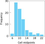
![]() FIGURE 8.9 Surface roughness in microinches for a machined part.
FIGURE 8.9 Surface roughness in microinches for a machined part.
![]() FIGURE 8.10 Reciprocals of surface roughness. (Adapted from data in the “Statistics Corner” column in Quality Progress, March 1989, with permission of the American Society for Quality.)
FIGURE 8.10 Reciprocals of surface roughness. (Adapted from data in the “Statistics Corner” column in Quality Progress, March 1989, with permission of the American Society for Quality.)
Other approaches have been considered in dealing with non-normal data. There have been various attempts to extend the definitions of the standard capability indices to the case of non-normal distributions. Luceño (1996) introduced the index Cpc, defined as

where the process target value ![]() . Luceño uses the second subscript in Cpc to stand for confidence, and he stresses that the confidence intervals based on Cpc are reliable; of course, this statement should be interpreted cautiously. The author has also used the constant
. Luceño uses the second subscript in Cpc to stand for confidence, and he stresses that the confidence intervals based on Cpc are reliable; of course, this statement should be interpreted cautiously. The author has also used the constant ![]() in the denominator, to make it equal to 6σ when the underlying distribution is normal. We will give the confidence interval for Cpc in Section 8.3.5.
in the denominator, to make it equal to 6σ when the underlying distribution is normal. We will give the confidence interval for Cpc in Section 8.3.5.
There have also been attempts to modify the usual capability indices so that they are appropriate for two general families of distributions: the Pearson and Johnson families. This would make PCRs broadly applicable for both normal and non-normal distributions. Good discussions of these approaches are in Rodriguez (1992) and Kotz and Lovelace (1998).
The general idea is to use appropriate quantiles of the process distribution—say, x0.00135 and x0.99865—to define a quantile-based PCR—say,
Now since in the normal distribution x0.00135 = μ – 3μ and x0.99865 = μ + 3σ, we see that in the case of a normal distribution Cp(q) reduces to Cp. Clements (1989) proposed a method for determining the quantiles based on the Pearson family of distributions. In general, however, we could fit any distribution to the process data, determine its quantiles x0.99865 and x0.00135, and apply equation 8.11. Refer to Kotz and Lovelace (1998) for more information.
8.3.4 More about Process Centering
The process capability ratio Cpk was initially developed because Cp does not adequately deal with the case of a process with mean μ that is not centered between the specification limits. However, Cpk alone is still an inadequate measure of process centering. For example, consider the two processes shown in Figure 8.11. Both processes A and B have Cpk = 1.0, yet their centering is clearly different. To characterize process centering satisfactorily, Cpk must be compared to Cp. For process A, Cpk = Cp = 1.0, implying that the process is centered, whereas for process B, Cp = 2.0 > Cpk = 1.0, implying that the process is off center. For any fixed value of μ in the interval from LSL to USL, Cpk depends inversely on σ and becomes large as σ approaches zero. This characteristic can make Cpk unsuitable as a measure of centering. That is, a large value of Cpk does not really tell us anything about the location of the mean in the interval from LSL to USL.

![]() FIGURE 8.11 Two processes with Cpk = 1.0.
FIGURE 8.11 Two processes with Cpk = 1.0.
One way to address this difficulty is to use a process capability ratio that is a better indicator of centering. PCR Cpm is one such ratio, where
and τ is the square root of expected squared deviation from target ![]() ,
,
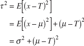
Thus, equation 8.12 can be written as

where
A logical way to estimate Cpm is by
where
Chan, Cheng, and Spiring (1988) discussed this ratio, various estimators of Cpm, and their sampling properties. Boyles (1991) has provided a definitive analysis of Cpm and its usefulness in measuring process centering. He notes that both Cpk and Cpm coincide with Cp when μ = T and decrease as μ moves away from T. However, Cpk < 0 for μ > USL or μ < LSL, whereas Cpm approaches zero asymptotically as |(μ – T)| → ∞. Boyles also shows that the Cpm of a process with |(μ – T)| = Δ > 0 is strictly bounded above by the Cp value of a process with σ = Δ. That is,
Thus, a necessary condition for Cpm ≥ 1 is
![]()
This statistic says that if the target value T is the midpoint of the specifications, a Cpm of one or greater implies that the mean μ lies within the middle third of the specification band. A similar statement can be made for any value of Cpm. For instance, ![]() implies that
implies that ![]() . Thus, a given value of Cpm places a constraint on the difference between μ and the target value T.
. Thus, a given value of Cpm places a constraint on the difference between μ and the target value T.
To illustrate the use of Cpm, consider the two processes A and B in Figure 8.11. For process A we find that
![]()
since process A is centered at the target value T = 50. Note that Cpm = Cpk for process A. Now consider process B:
![]()
If we use equation 8.17, this is equivalent to saying that the process mean lies approximately within the middle half of the specification range. Visual examination of Figure 8.11 reveals this to be the case.
Pearn et al. (1992) proposed the process capability ratio

This is sometimes called a “third generation” process capability ratio, since it is constructed from the “second generation” ratios Cpk and Cpm in the same way that they were generated from the “first generation” ratio Cp. The motivation of this new ratio is increased sensitivity to departures of the process mean μ from the desired target T. For more details, see Kotz and Lovelace (1998).
8.3.5 Confidence Intervals and Tests on Process Capability Ratios
Confidence Intervals on Process Capability Ratios. Much of the industrial use of process capability ratios focuses on computing and interpreting the point estimate of the desired quantity. It is easy to forget that ![]() or
or ![]() (for examples) are simply point estimates, and, as such, are subject to statistical fluctuation. An alternative that should become standard practice is to report confidence intervals for process capability ratios.
(for examples) are simply point estimates, and, as such, are subject to statistical fluctuation. An alternative that should become standard practice is to report confidence intervals for process capability ratios.
It is easy to find a confidence interval for the “first generation” ratio Cp. If we replace σ by s in the equation for Cp, we produce the usual point estimator ![]() . If the quality characteristic follows a normal distribution, then a 100(1 – α)% CI on Cp is obtained from
. If the quality characteristic follows a normal distribution, then a 100(1 – α)% CI on Cp is obtained from
or

where ![]() and
and ![]() are the lower α/2 and upper α/2 percentage points of the chi-square distribution with n – 1 degrees of freedom. These percentage points are tabulated in Appendix Table III.
are the lower α/2 and upper α/2 percentage points of the chi-square distribution with n – 1 degrees of freedom. These percentage points are tabulated in Appendix Table III.
EXAMPLE 8.4 A Confidence Interval in Cp
Suppose that a stable process has upper and lower specifications at USL = 62 and LSL = 38. A sample of size n = 20 from this process reveals that the process mean is centered approximately at the midpoint of the specification interval and that the sample standard deviation s = 1.75. Find a 95% CI on Cp.
SOLUTION
A point estimate of Cp is
![]()
The 95% confidence interval on Cp is found from equation 8.20 as follows:
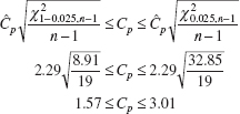
where ![]() and
and ![]() were taken from Appendix Table III.
were taken from Appendix Table III.
The confidence interval on Cp in Example 8.4 is relatively wide because the sample standard deviation s exhibits considerable fluctuation in small to moderately large samples. This means, in effect, that confidence intervals on Cp based on small samples will be wide.
Note also that the confidence interval uses s rather than ![]() to estimate σ. This further emphasizes that the process must be in statistical control for PCRs to have any real meaning. If the process is not in control, s and
to estimate σ. This further emphasizes that the process must be in statistical control for PCRs to have any real meaning. If the process is not in control, s and ![]() could be very different, leading to very different values of the PCR.
could be very different, leading to very different values of the PCR.
For more complicated ratios such as Cpk and Cpm, various authors have developed approximate confidence intervals; for example, see Zhang, Stenback, and Wardrop (1990), Bissell (1990), Kushler and Hurley (1992), and Pearn et al. (1992). If the quality characteristic is normally distributed, then an approximate 100(1 – α)% CI on Cpk is given as follows.
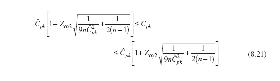
Kotz and Lovelace (1998) give an extensive summary of confidence intervals for various PCRs.
EXAMPLE 8.5 A Confidence Interval on Cpk
A sample of size n = 20 from a stable process is used to estimate Cpk, with the result that ![]() . Find an approximate 95% CI on Cpk.
. Find an approximate 95% CI on Cpk.
SOLUTION
Using equation 8.21, an approximate 95% CI on Cpk is

or
![]()
This is an extremely wide confidence interval. Based on the sample data, the ratio Cpk could be less than 1 (a very bad situation), or it could be as large as 1.78 (a reasonably good situation). Thus, we have learned very little about actual process capability, because Cpk is very imprecisely estimated. The reason for this, of course, is that a very small sample (n = 20) has been used.
For non-normal data, the PCR Cpc developed by Luceño (1996) can be employed. Recall that Cpc was defined in equation 8.10. Luceño developed the confidence interval for Cpc as follows: First, evaluate |(x – T)|, whose expected value is estimated by
![]()
leading to the estimator

A 100(1 – α)% CI for E|(x – T)| is given as
![]()
where
![]()
Therefore, a 100(1 – α)% confidence interval for Cpc is given by

Testing Hypotheses about PCRs. A practice that is becoming increasingly common in industry is to require a supplier to demonstrate process capability as part of the contractual agreement. Thus, it is frequently necessary to demonstrate that the process capability ratio Cp meets or exceeds some particular target value—say, Cp0. This problem may be formulated as a hypothesis testing problem:
![]()
We would like to reject H0 (recall that in statistical hypothesis testing rejection of H0 is always a strong conclusion), thereby demonstrating that the process is capable. We can formulate the statistical test in terms of ![]() , so that we will reject H0 if
, so that we will reject H0 if ![]() exceeds a critical value C.
exceeds a critical value C.
Kane (1986) has investigated this test, and provides a table of sample sizes and critical values for C to assist in testing process capability. We may define Cp (High) as a process capability that we would like to accept with probability 1 – α and Cp (Low) as a process capability that we would like to reject with probability 1 – β. Table 8.4 gives values of Cp(High)/Cp(Low) and C/Cp(Low) for varying sample sizes and α = β = 0.05 or α = β = 0.10. Example 8.6 illustrates the use of this table.
EXAMPLE 8.6 Supplier Qualification
A customer has told his supplier that, in order to qualify for business with his company, the supplier must demonstrate that his process capability exceeds Cp = 1.33. Thus, the supplier is interested in establishing a procedure to test the hypotheses
![]()
The supplier wants to be sure that if the process capability is below 1.33 there will be a high probability of detecting this (say, 0.90), whereas if the process capability exceeds 1.66 there will be a high probability of judging the process capable (again, say, 0.90). This would imply that Cp(Low) = 1.33, Cp(High) = 1.66, and α = β = 0.10. To find the sample size and critical value for C from Table 8.4, compute
![]()
![]() TABLE 8.4
TABLE 8.4
Sample Size and Critical Value Determination for Testing H0: Cp = Cp0
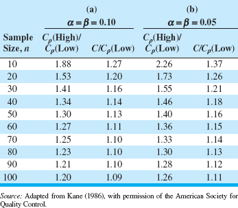
and enter the table value in panel (a) where α = β = 0.10. This yields
n = 70
and
C/Cp(Low) = 1.10
from which we calculate
C = Cp(Low)1.10 = 1.33(1.10) = 1.46
Thus, to demonstrate capability, the supplier must take a sample of n = 70 parts, and the sample process capability ratio ![]() must exceed C ≤ 1.46.
must exceed C ≤ 1.46.
This example shows that, in order to demonstrate that process capability is at least equal to 1.33, the observed sample ![]() will have to exceed 1.33 by a considerable amount. This illustrates that some common industrial practices may be questionable statistically. For example, it is fairly common practice to accept the process as capable at the level Cp ≥ 1.33 if the sample
will have to exceed 1.33 by a considerable amount. This illustrates that some common industrial practices may be questionable statistically. For example, it is fairly common practice to accept the process as capable at the level Cp ≥ 1.33 if the sample ![]() ≥ 1.33 based on a sample size of 30 ≤ n ≤ 50 parts. Clearly, this procedure does not account for sampling variation in the estimate of σ, and larger values of n and/or higher acceptable values of
≥ 1.33 based on a sample size of 30 ≤ n ≤ 50 parts. Clearly, this procedure does not account for sampling variation in the estimate of σ, and larger values of n and/or higher acceptable values of ![]() may be necessary in practice.
may be necessary in practice.
Process Performance Indices. In 1991, the Automotive Industry Action Group (AIAG) was formed and consists of representatives of the “big three” (Ford, General Motors, and Chrysler) and the American Society for Quality Control (now the American Society for Quality). One of their objectives was to standardize the reporting requirements from suppliers and in general of their industry. The AIAG recommends using the process capability indices Cp and Cpk when the process is in control, with the process standard deviation estimated by ![]() . When the process is not in control, the AIAG recommends using process performance indices Pp and Ppk, where, for example,
. When the process is not in control, the AIAG recommends using process performance indices Pp and Ppk, where, for example,
![]()
and s is the usual sample standard deviation ![]() . Even the American National Standards Institute in ANSI Standard Z1 on Process Capability Analysis (1996) states that Pp and Ppk should be used when the process is not in control.
. Even the American National Standards Institute in ANSI Standard Z1 on Process Capability Analysis (1996) states that Pp and Ppk should be used when the process is not in control.
Now it is clear that when the process is normally distributed and in control, ![]() is essentially
is essentially ![]() and
and ![]() is essentially
is essentially ![]() because for a stable process the difference between s and
because for a stable process the difference between s and ![]() is minimal. However, please note that if the process is not in control, the indices Pp and Ppk have no meaningful interpretation relative to process capability, because they cannot predict process performance. Furthermore, their statistical properties are not determinable, and so no valid inference can be made regarding their true (or population) values. Also, Pp and Ppk provide no motivation or incentive to the companies that use them to bring their processes into control.
is minimal. However, please note that if the process is not in control, the indices Pp and Ppk have no meaningful interpretation relative to process capability, because they cannot predict process performance. Furthermore, their statistical properties are not determinable, and so no valid inference can be made regarding their true (or population) values. Also, Pp and Ppk provide no motivation or incentive to the companies that use them to bring their processes into control.
Kotz and Lovelace (1998) strongly recommend against the use of Pp and Ppk, indicating that these indices are actually a step backward in quantifying process capability. They refer to the mandated use of Pp and Ppk through quality standards or industry guidelines as undiluted “statistical terrorism” (i.e., the use or misuse of statistical methods along with threats and/or intimidation to achieve a business objective).
This author agrees completely with Kotz and Lovelace. The process performance indices Pp and Ppk are actually more than a step backward. They are a waste of engineering and management effort—they tell you nothing. Unless the process is stable (in control), no index is going to carry useful predictive information about process capability or convey any information about future performance. Instead of imposing the use of meaningless indices, organizations should devote effort to developing and implementing an effective process characterization, control, and improvement plan. This is a much more reasonable and effective approach to process improvement.
8.4 Process Capability Analysis Using a Control Chart
Histograms, probability plots, and process capability ratios summarize the performance of the process. They do not necessarily display the potential capability of the process because they do not address the issue of statistical control, or show systematic patterns in process output that, if eliminated, would reduce the variability in the quality characteristic. Control charts are very effective in this regard. The control chart should be regarded as the primary technique of process capability analysis.
Both attributes and variables control charts can be used in process capability analysis. The ![]() and R charts should be used whenever possible, because of the greater power and better information they provide relative to attributes charts. However, both p charts and c (or u) charts are useful in analyzing process capability. Techniques for constructing and using these charts are given in Chapters 6 and 7. Remember that to use the p chart there must be specifications on the product characteristics. The
and R charts should be used whenever possible, because of the greater power and better information they provide relative to attributes charts. However, both p charts and c (or u) charts are useful in analyzing process capability. Techniques for constructing and using these charts are given in Chapters 6 and 7. Remember that to use the p chart there must be specifications on the product characteristics. The ![]() and R charts allow us to study processes without regard to specifications.
and R charts allow us to study processes without regard to specifications.
The ![]() and R control charts allow both the instantaneous variability (short-term process capability) and variability across time (long-term process capability) to be analyzed. It is particularly helpful if the data for a process capability study are collected in two to three different time periods (such as different shifts, different days, etc.).
and R control charts allow both the instantaneous variability (short-term process capability) and variability across time (long-term process capability) to be analyzed. It is particularly helpful if the data for a process capability study are collected in two to three different time periods (such as different shifts, different days, etc.).
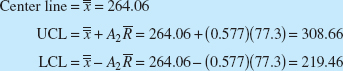
Table 8.5 presents the container bursting-strength data in 20 samples of five observations each. The calculations for the ![]() and R charts are summarized here:
and R charts are summarized here:
![]() Chart
Chart
R Chart
Center line = ![]() = 77.3
= 77.3
![]()
Figure 8.12 presents the ![]() and R charts for the 20 samples in Table 8.5. Both charts exhibit statistical control. The process parameters may be estimated from the control chart as
and R charts for the 20 samples in Table 8.5. Both charts exhibit statistical control. The process parameters may be estimated from the control chart as

![]() TABLE 8.5
TABLE 8.5
Glass Container Strength Data (psi)

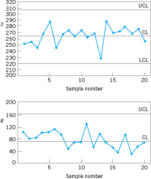
![]() FIGURE 8.12
FIGURE 8.12 ![]() and R charts for the bottle-strength data.
and R charts for the bottle-strength data.
Thus, the one-sided lower process capability ratio is estimated by
![]()
Clearly, since strength is a safety-related parameter, the process capability is inadequate.
This example illustrates a process that is in control but operating at an unacceptable level. There is no evidence to indicate that the production of nonconforming units is operator-controllable. Engineering and/or management intervention will be required either to improve the process or to change the requirements if the quality problems with the bottles are to be solved. The objective of these interventions is to increase the process capability ratio to at least a minimum acceptable level. The control chart can be used as a monitoring device or logbook to show the effect of changes in the process on process performance.
Sometimes the process capability analysis indicates an out-of-control process. It is unsafe to estimate process capability in such cases. The process must be stable in order to produce a reliable estimate of process capability. When the process is out of control in the early stages of process capability analysis, the first objective is finding and eliminating the assignable causes in order to bring the process into an in-control state.
8.5 Process Capability Analysis Using Designed Experiments
A designed experiment is a systematic approach to varying the input controllable variables in the process and analyzing the effects of these process variables on the output. Designed experiments are also useful in discovering which set of process variables is influential on the output, and at what levels these variables should be held to optimize process performance. Thus, design of experiments is useful in more general problems than merely estimating process capability. For an introduction to design of experiments, see Montgomery (2009). Part V of this textbook provides more information on experimental design methods and on their use in process improvement.
One of the major uses of designed experiments is in isolating and estimating the sources of variability in a process. For example, consider a machine that fills bottles with a soft-drink beverage. Each machine has a large number of filling heads that must be independently adjusted. The quality characteristic measured is the syrup content (in degrees brix) of the finished product. There can be variation in the observed brix (![]() ) because of machine variability (
) because of machine variability (![]() ), head variability (
), head variability (![]() ), and analytical test variability (
), and analytical test variability (![]() ). The variability in the observed brix value is
). The variability in the observed brix value is
![]()
An experiment can be designed, involving sampling from several machines and several heads on each machine, and making several analyses on each bottle, which would allow estimation of the variances (![]() ), (
), (![]() ), and (
), and (![]() ). Suppose that the results appear as in Figure 8.13. Since a substantial portion of the total variability in observed brix is due to variability among heads, this indicates that the process can perhaps best be improved by reducing the head-to-head variability. This could be done by more careful setup or by more careful control of the operation of the machine.
). Suppose that the results appear as in Figure 8.13. Since a substantial portion of the total variability in observed brix is due to variability among heads, this indicates that the process can perhaps best be improved by reducing the head-to-head variability. This could be done by more careful setup or by more careful control of the operation of the machine.

![]() FIGURE 8.13 Sources of variability in the bottling line example.
FIGURE 8.13 Sources of variability in the bottling line example.
8.6 Process Capability Analysis with Attribute Data
Often process performance is measured in terms of attribute data—that is, nonconforming units or defectives, or nonconformities or defects. When a fraction nonconforming is the measure of performance, it is typical to use the parts per million (ppm) defective as a measure of process capability. In some organizations, this ppm defective is converted to an equivalent sigma level. For example, a process producing 2,700 ppm defective would be equivalent to a three-sigma process (without the “usual” 1.5 σ shift in the mean that many Six Sigma organizations employ in the calculations taken into account).
When dealing with nonconformities or defects, a defects per unit (DPU) statistic is often used as a measure of capability, where
![]()
Here the unit is something that is delivered to a customer and can be evaluated or judged as to its suitability. Some examples include:
1. An invoice
2. A shipment
3. A customer order
4. An enquiry or call
The defects or nonconformities are anything that does not meet the customer requirements, such as:
1. An error on an invoice
2. An incorrect or incomplete shipment
3. An incorrect or incomplete customer order
4. A call that is not satisfactorily completed
Obviously, these quantities are estimated from sample data. Large samples need to be used to obtain reliable estimates.
The DPU measure does not directly take the complexity of the unit into account. A widely used way to do this is the defect per million opportunities (DPMO) measure
![]()
Opportunities are the number of potential chances within a unit for a defect to occur. For example, on a purchase order, the number of opportunities would be the number of fields in which information is recorded times two, because each field can either be filled out incorrectly or blank (information is missing). It is important to be consistent about how opportunities are defined, as a process may be artificially improved simply by increasing the number of opportunities over time.
8.7 Gauge and Measurement System Capability Studies
8.7.1 Basic Concepts of Gauge Capability
Determining the capability of the measurement system is an important aspect of many quality and process improvement activities. Generally, in any activity involving measurements, some of the observed variability will be inherent in the units or items that are being measured, and some of the variability will result from the measurement system that is used. The measurement system will consist (minimally) of an instrument or gauge, and it often has other components, such as the operator(s) that uses it and the conditions or different points in time under which the instrument is used. There may also be other factors that impact measurement system performance, such as setup or calibration activities. The purpose of most measurement systems capability studies is to:
1. Determine how much of the total observed variability is due to the gauge or instrument
2. Isolate the components of variability in the measurement system
3. Assess whether the instrument or gauge is capable (that is, is it suitable for the intended application)
Measurements are a significant component of any quality system. Measurement is an integral component of the DMAIC problem-solving process, but it’s even more important than that. An ineffective measurement system can dramatically impact business performance because it leads to uninformed (and usually bad) decision making.
In this section we will introduce the two R’s of measurement systems capability: repeatability (Do we get the same observed value if we measure the same unit several times under identical conditions?), and reproducibility (How much difference in observed values do we experience when units are measured under different conditions, such as different operators, time periods, and so forth?).
These quantities answer only indirectly the fundamental question: Is the system able to distinguish between good and bad units? That is, what is the probability that a good unit is judged to be defective and, conversely, that a bad unit is passed along to the customer as good? These misclassification probabilities are fairly easy to calculate from the results of a standard measurement systems capability study, and give reliable, useful, and easy-to-understand information about measurement systems performance.
In addition to repeatability and reproducibility, there are other important aspects of measurement systems capability. The linearity of a measurement system reflects the differences in observed accuracy and/or precision experienced over the range of measurements made by the system. A simple linear regression model is often used to describe this feature. Problems with linearity are often the result of calibration and maintenance issues. Stability, or different levels of variability in different operating regimes, can result from warm-up effects, environmental factors, inconsistent operator performance, and inadequate standard operating procedure. Bias reflects the difference between observed measurements and a “true” value obtained from a master or gold standard, or from a different measurement technique known to produce accurate values.
It is very difficult to monitor, control, improve, or effectively manage a process with an inadequate measurement system. It’s somewhat analogous to navigating a ship through fog without radar—eventually you are going to hit the iceberg! Even if no catastrophe occurs, you always are going to be wasting time and money looking for problems where none exist and dealing with unhappy customers who received defective product. Because excessive measurement variability becomes part of overall product variability, it also negatively impacts many other process improvement activities, such as leading to larger sample sizes in comparative or observational studies, more replication in designed experiments aimed at process improvement, and more extensive product testing.
To introduce some of the basic ideas of measurement systems analysis (MSA), consider a simple but reasonable model for measurement system capability studies
where y is the total observed measurement, x is the true value of the measurement on a unit of product, and e is the measurement error. We will assume that x and ε are normally and independently distributed random variables with means μ and 0 and variances (![]() ) and (
) and (![]() ), respectively. The variance of the total observed measurement, y, is then
), respectively. The variance of the total observed measurement, y, is then

Control charts and other statistical methods can be used to separate these components of variance, as well as to give an assessment of gauge capability.
EXAMPLE 8.7 Measuring Gauge Capability
An instrument is to be used as part of a proposed SPC implementation. The quality-improvement team involved in designing the SPC system would like to get an assessment of gauge capability. Twenty units of the product are obtained, and the process operator who will actually take the measurements for the control chart uses the instrument to measure each unit of product twice. The data are shown in Table 8.6.
SOLUTION
Figure 8.14 shows the ![]() and R charts for these data. Note that the
and R charts for these data. Note that the ![]() chart exhibits many out-of-control points. This is to be expected, because in this situation the
chart exhibits many out-of-control points. This is to be expected, because in this situation the ![]() chart has an interpretation that is somewhat different from the usual interpretation. The
chart has an interpretation that is somewhat different from the usual interpretation. The ![]() chart in this example shows the discriminating power of the instrument—literally, the ability of the gauge to distinguish between units of product. The R chart directly shows the magnitude of measurement error, or the gauge capability. The R values represent the difference between measurements made on the same unit using the same instrument. In this example, the R chart is in control. This indicates that the operator is having no difficulty in making consistent measurements. Out-of-control points on the R chart could indicate that the operator is having difficulty using the instrument.
chart in this example shows the discriminating power of the instrument—literally, the ability of the gauge to distinguish between units of product. The R chart directly shows the magnitude of measurement error, or the gauge capability. The R values represent the difference between measurements made on the same unit using the same instrument. In this example, the R chart is in control. This indicates that the operator is having no difficulty in making consistent measurements. Out-of-control points on the R chart could indicate that the operator is having difficulty using the instrument.
The standard deviation of measurement error, σGauge, can be estimated as follows:
![]()
The distribution of measurement error is usually well approximated by the normal. Thus, ![]() is a good estimate of gauge capability.
is a good estimate of gauge capability.
![]() TABLE 8.6
TABLE 8.6
Parts Measurement Data


![]() FIGURE 8.14 Control charts for the gauge capability analysis in Example 8.7.
FIGURE 8.14 Control charts for the gauge capability analysis in Example 8.7.
It is a fairly common (but not necessarily good) practice to compare the estimate of gauge capability to the width of the specifications or the tolerance band (USL – LSL) for the part that is being measured. The ratio of k![]() to the total tolerance band is often called the precision-to-tolerance (P/T) ratio:
to the total tolerance band is often called the precision-to-tolerance (P/T) ratio:

In equation 8.25, popular choices for the constant k are k = 5.15 and k = 6. The value k = 5.15 corresponds to the limiting value of the number of standard deviations between bounds of a 95% tolerance interval that contains at least 99% of a normal population, and k = 6 corresponds to the number of standard deviations between the usual natural tolerance limits of a normal population.
The part used in Example 8.7 has USL = 60 and LSL = 5. Therefore, taking k = 6 in equation 8.25, an estimate of the P/T ratio is
![]()
Values of the estimated ratio P/T of 0.1 or less often are taken to imply adequate gauge capability. This is based on the generally used rule that requires a measurement device to be calibrated in units one-tenth as large as the accuracy required in the final measurement. However, we should use caution in accepting this general rule of thumb in all cases. A gauge must be sufficiently capable of measuring product accurately enough and precisely enough so that the analyst can make the correct decision. This may not necessarily require that P/T ≤ 0.1.
We can use the data from the gauge capability experiment in Example 8.7 to estimate the variance components in equation 8.24 associated with total observed variability. From the actual sample measurements in Table 8.6, we can calculate s = 3.17. This is an estimate of the standard deviation of total variability, including both product variability and gauge variability. Therefore,
![]()
Since from equation 8.24 we have
![]()
and because we have an estimate of ![]() , we can obtain an estimate of
, we can obtain an estimate of ![]() as
as
![]()
Therefore, an estimate of the standard deviation of the product characteristic is
![]()
There are other measures of gauge capability that have been proposed. One of these is the ratio of process (part) variability to total variability:
and another is the ratio of measurement system variability to total variability:
Obviously, ρP = 1 – ρM. For the situation in Example 8.7 we can calculate an estimate of ρM as follows:
![]()
Thus the variance of the measuring instrument contributes about 7.86% of the total observed variance of the measurements.
Another measure of measurement system adequacy is defined by the AIAG (1995) [note that there is also on updated edition of this manual, AIAG (2002)] as the signal-to-noise ratio (SNR):
AIAG defined the SNR as the number of distinct levels or categories that can be reliably obtained from the measurements. A value of 5 or greater is recommended, and a value of less than 2 indicates inadequate gauge capability. For Example 8.7 we have ![]() , and using
, and using ![]() we find that
we find that ![]() , so an estimate of the SNR in equation 8.28 is
, so an estimate of the SNR in equation 8.28 is
![]()
Therefore, the gauge in Example 8.7 would not meet the suggested requirement of an SNR of at least 5. However, this requirement on the SNR is somewhat arbitrary. Another measure of gauge capability is the discrimination ratio (DR)
Some authors have suggested that for a gauge to be capable the DR must exceed 4. This is a very arbitrary requirement. For the situation in Example 8.7, we would calculate an estimate of the discrimination ratio as
![]()
Clearly by this measure, the gauge is capable.
Finally, in this section we have focused primarily on instrument or gauge precision, not gauge accuracy. These two concepts are illustrated in Figure 8.15. In this figure, the bull’s-eye of the target is considered to be the true value of the measured characteristic, or μ the mean of x in equation 8.23. Accuracy refers to the ability of the instrument to measure the true value correctly on average, whereas precision is a measure of the inherent variability in the measurement system. Evaluating the accuracy of a gauge or measurement system often requires the use of a standard, for which the true value of the measured characteristic is known. Often the accuracy feature of an instrument can be modified by making adjustments to the instrument or by the use of a properly constructed calibration curve.
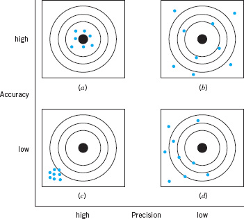
![]() FIGURE 8.15 The concepts of accuracy and precision. (a) The gauge is accurate and precise. (b) The gauge is accurate but not precise. (c) The gauge is not accurate but it is precise. (d) The gauge is neither accurate nor precise.
FIGURE 8.15 The concepts of accuracy and precision. (a) The gauge is accurate and precise. (b) The gauge is accurate but not precise. (c) The gauge is not accurate but it is precise. (d) The gauge is neither accurate nor precise.
It is also possible to design measurement systems capability studies to investigate two components of measurement error, commonly called the repeatability and the reproducibility of the gauge. We define reproducibility as the variability due to different operators using the gauge (or different time periods, or different environments, or in general, different conditions) and repeatability as reflecting the basic inherent precision of the gauge itself. That is,

The experiment used to measure the components of ![]() is usually called a gauge R & R study, for the two components of
is usually called a gauge R & R study, for the two components of ![]() . We now show how to analyze gauge R & R experiments.
. We now show how to analyze gauge R & R experiments.
8.7.2 The Analysis of Variance Method
An example of a gauge R & R study, taken from the paper by Houf and Berman (1988) is shown in Table 8.7. The data are measurements on thermal impedance (in degrees C per Watt × 100) on a power module for an induction motor starter. There are 10 parts, 3 operators, and 3 measurements per part. The gauge R & R study is a designed experiment. Specifically, it is a factorial experiment, so-called because each inspector or “operator” measures all of the parts.
The analysis of variance introduced in Chapter 9 can be extended to analyze the data from a gauge R & R experiment and to estimate the appropriate components of measurement systems variability. We give only an introduction to the procedure here; for more details, see Montgomery (2009), Montgomery and Runger (1993a, 1993b), Borror, Montgomery, and Runger (1997), Burdick and Larsen (1997), the review paper by Burdick, Borror, and Montgomery (2003), the book by Burdick, Borror, and Montgomery (2005), and the supplemental text material for this chapter.
![]() TABLE 8.7
TABLE 8.7
Thermal Impedance Data (°C/W × 100) for the Gauge R & R Experiment

If there are a randomly selected parts and b randomly selected operators, and each operator measures every part n times, then the measurements (i = part, j = operator, k = measurement) could be represented by the model
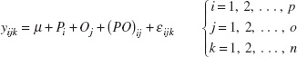
where the model parameters Pi, Oj, (PO)ij, and εijk are all independent random variables that represent the effects of parts, operators, the interaction or joint effects of parts and operators, and random error. This is a random effects model analysis of variance (ANOVA). It is also sometimes called the standard model for a gauge R & R experiment. We assume that the random variables Pi, Oj, (PO)ij, and εijk are normally distributed with mean zero and variances given by ![]() , and V(εijk) = σ2. Therefore, the variance of any observation is
, and V(εijk) = σ2. Therefore, the variance of any observation is
and ![]() , and σ2 are the variance components. We want to estimate the variance components.
, and σ2 are the variance components. We want to estimate the variance components.
Analysis of variance methods can be used to estimate the variance components. The procedure involves partitioning the total variability in the measurements into the following component parts:
where, as in Chapter 4, the notation SS represents a sum of squares. Although these sums of squares could be computed manually,1 in practice we always use a computer software package to perform this task. Each sum of squares on the right-hand side of equation 8.32 is divided by its degrees of freedom to produce mean squares:

We can show that the expected values of the mean squares are as follows:
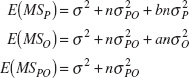
E(MSE) = σ2
The variance components may be estimated by equating the calculated numerical values of the mean squares from an analysis of the variance computer program to their expected values and solving for the variance components. This yields
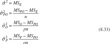
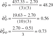
Table 8.8 shows the analysis of variance for this experiment. The computations were performed using the Balanced ANOVA routine in Minitab. Based on the P-values, we conclude that the effect of parts is large, operators may have a small effect, and there is no significant part-operator interaction. We may use equation 8.33 to estimate the variance components as follows:
![]() TABLE 8.8
TABLE 8.8
ANOVA: Thermal Impedance versus Part Number, Operator
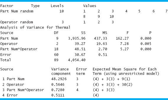
![]()
Note that these estimates also appear at the bottom of the Minitab output.
Occasionally we will find that the estimate of one of the variance components will be negative. This is certainly not reasonable, since by definition variances are nonnegative. Unfortunately, negative estimates of variance components can result when we use the analysis of variance method of estimation (this is considered one of its drawbacks). There are a variety of ways to deal with this. One possibility is to assume that the negative estimate means that the variance component is really zero and just set it to zero, leaving the other nonnegative estimates unchanged. Another approach is to estimate the variance components with a method that ensures nonnegative estimates. Finally, when negative estimates of variance components occur, they are usually accompanied by nonsignificant model sources of variability. For example, if ![]() is negative, it will usually be because the interaction source of variability is nonsignificant. We should take this as evidence that
is negative, it will usually be because the interaction source of variability is nonsignificant. We should take this as evidence that ![]() really is zero, that there is no interaction effect, and fit a reduced model of the form
really is zero, that there is no interaction effect, and fit a reduced model of the form
yijk = μ + Pi + Oj + εijk
that does not include the interaction term. This is a relatively easy approach and one that often works nearly as well as more sophisticated methods.
Typically we think of σ2 as the repeatability variance component, and the gauge reproducibility as the sum of the operator and the part × operator variance components,
![]()
Therefore
![]()
and the estimate for our example is

The lower and upper specifications on this power module are LSL = 18 and USL = 58. Therefore the P/T ratio for the gauge is estimated as
![]()
By the standard measures of gauge capability, this gauge would not be considered capable because the estimate of the P/T ratio exceeds 0.10.
8.7.3 Confidence Intervals in Gauge R & R Studies
The gauge R & R study and the ANOVA procedure described in the previous section resulted in point estimates of the experimental model variance components and for ![]() . It can be very informative to obtain confidence intervals for gauge R & R studies. Confidence intervals in measurement systems capability studies are discussed in Montgomery (2001), Montgomery and Runger (1993a, 1993b), Borror, Montgomery, and Runger (1997), Burdick and Larsen (1997), the review paper by Burdick, Borror, and Montgomery (2003) and the book by Burdick, Borror, and Montgomery (2005). Among the different methods for obtaining these confidence intervals, the modified large sample (MLS) method produces good results and is relatively easy to implement for the standard gauge capability experiment described in Section 8.7.2, where both parts and operators are considered to be random factors. Other methods for constructing confidence intervals and computer programs to implement these methods are in Burdick, Borror, and Montgomery (2005).
. It can be very informative to obtain confidence intervals for gauge R & R studies. Confidence intervals in measurement systems capability studies are discussed in Montgomery (2001), Montgomery and Runger (1993a, 1993b), Borror, Montgomery, and Runger (1997), Burdick and Larsen (1997), the review paper by Burdick, Borror, and Montgomery (2003) and the book by Burdick, Borror, and Montgomery (2005). Among the different methods for obtaining these confidence intervals, the modified large sample (MLS) method produces good results and is relatively easy to implement for the standard gauge capability experiment described in Section 8.7.2, where both parts and operators are considered to be random factors. Other methods for constructing confidence intervals and computer programs to implement these methods are in Burdick, Borror, and Montgomery (2005).
Table 8.9 contains the MLS confidence interval equations for the parameters that are usually of interest in a measurement systems capability study. Definitions of the quantities used in Table 8.9 are in Table 8.10. References for all of the confidence interval equations in Table 8.9 are in Burdick, Borror, and Montgomery (2003). Note that the percentage point of the F distribution defined in Table 8.10 as Fα,df,∞ = χ2α,df.
The last column in Table 8.9 contains the 95% confidence intervals for each parameter, and the last column of Table 8.10 shows the numerical values of the quantities used in computing the 95% confidence intervals. All of the confidence intervals in Table 8.9 are fairly wide because there are only three operators, and this results in only two degrees of freedom to estimate the operator effect. Therefore, this will have an impact on length of any confidence interval for any parameter that is a function of ![]() . This suggests that to obtain narrower confidence intervals in a gauge R & R study, it will be necessary to increase the number of operators. Since it is fairly standard practice to use only two or three operators in these studies, this implies that one needs to carefully consider the consequences of applying a standard design to estimate gauge capability.
. This suggests that to obtain narrower confidence intervals in a gauge R & R study, it will be necessary to increase the number of operators. Since it is fairly standard practice to use only two or three operators in these studies, this implies that one needs to carefully consider the consequences of applying a standard design to estimate gauge capability.
8.7.4 False Defectives and Passed Defectives
In previous sections we have introduced several ways to summarize the capability of a gauge or instrument, including the P/T ratio (equation 8.25), the signal-to-noise ratio SNR (equation 8.28), the discrimination ratio DR (equation 8.29), and ρP and ρM (equations 8.26 and 8.27). None of these quantities really describe the capability of the gauge in any sense that is directly interpretable. The effective capability of a measuring system is best described in terms of how well it discriminates between good and bad parts. Consider the model first proposed in equation 8.23:
![]() TABLE 8.9
TABLE 8.9
100(1 − α)% MLS Confidence Intervals for the Standard Gauge R & R Experiment
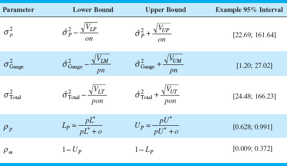
![]() TABLE 8.10
TABLE 8.10
Definition of Terms in Table 8.9

where y is the total observed measurement, x is the true value of the measurement, and e is the measurement error. The random variables x and ε are normally and independently distributed random variables with means μ and 0 and variances ![]() , respectively. The joint probability density function of y and x, say f (y, x), is bivariate normal with mean vector [μ, μ]′ and covariance matrix
, respectively. The joint probability density function of y and x, say f (y, x), is bivariate normal with mean vector [μ, μ]′ and covariance matrix
![]()
A unit of product or part is in conformance to the specifications if
and the measurement system will “pass” a unit as a nondefective if
If equation 8.34 is true but equation 8.35 is false, a conforming part has been incorrectly failed. Alternatively, if equation 8.34 is false but equation 8.35 is true, a nonconforming part has been incorrectly passed. Sometimes this is called a missed fault. A very useful way to describe the capability of a measurement system is in terms of producer’s risk and consumer’s risk. The producer’s risk δ is defined as the conditional probability that a measurement system will fail a part when the part conforms to the specifications (this is also called a false failure). The consumer’s risk β is defined as the conditional probability that a measurement system will pass a part when the part does not conform to the specifications (this is the missed fault described above).
Expressions are available for computing the two conditional probabilities:

and

where f (x) represents the marginal probability density function for x which is normal with mean μ and variance ![]() . Figure 8.16 shows the regions of false failures (FF) and missed faults (MF) on a density contour of the bivariate normal distribution. Thus, equations 8.36 and 8.37 can be used to compute δ and β for given values of μ,
. Figure 8.16 shows the regions of false failures (FF) and missed faults (MF) on a density contour of the bivariate normal distribution. Thus, equations 8.36 and 8.37 can be used to compute δ and β for given values of μ, ![]() , LSL, and USL. The SAS code to perform this computation is shown in Table 8.11.
, LSL, and USL. The SAS code to perform this computation is shown in Table 8.11.
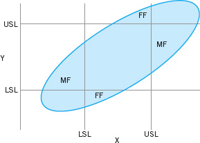
![]() FIGURE 8.16 Missed fault (MF) and false failures (FF) regions of a measurement system shown on a bivariate normal distribution contour. [From Burdick, Borror, and Montgomery (2003).]
FIGURE 8.16 Missed fault (MF) and false failures (FF) regions of a measurement system shown on a bivariate normal distribution contour. [From Burdick, Borror, and Montgomery (2003).]
In practice, we don’t know the true values of μ, ![]() , and
, and ![]() . If one uses only point estimates, the calculation does not account for the uncertainty in the estimates. It would be very helpful to provide confidence intervals for these parameters in the calculation of δ and β. One way to do this is to compute δ and β under different scenarios suggested by the confidence intervals on the variance components. For example, a pessimistic scenario might consider the worst possible performance for the measurement system, and the worst possible capability for the manufacturing process. To do this, set
. If one uses only point estimates, the calculation does not account for the uncertainty in the estimates. It would be very helpful to provide confidence intervals for these parameters in the calculation of δ and β. One way to do this is to compute δ and β under different scenarios suggested by the confidence intervals on the variance components. For example, a pessimistic scenario might consider the worst possible performance for the measurement system, and the worst possible capability for the manufacturing process. To do this, set ![]() equal to the upper bound of the confidence interval for
equal to the upper bound of the confidence interval for ![]() and solve for the value of
and solve for the value of ![]() that provides the lower bound on ρP. Conversely, one might consider an optimistic scenario with the best possible performance for the measurement system combined with the best process capability. For some other suggestions, see Burdick, Borror, and Montgomery (2003).
that provides the lower bound on ρP. Conversely, one might consider an optimistic scenario with the best possible performance for the measurement system combined with the best process capability. For some other suggestions, see Burdick, Borror, and Montgomery (2003).
Table 8.12 shows the calculation of the producer’s risk (δ) and the consumer’s risk (β) using equations 8.36 and 8.37 under the two scenarios discussed above. The scenario labeled “Pessimistic” is computed assuming the worst possible performance for both the production process and the measurement system. This is done by computing δ and β using the upper bound on ![]() and the lower bound on ρP. We used the sample mean 35.8 for the value of μ, the computed confidence bounds in Table 8.10, and solved for
and the lower bound on ρP. We used the sample mean 35.8 for the value of μ, the computed confidence bounds in Table 8.10, and solved for ![]() using the relationship
using the relationship ![]() . The SAS code shown in Table 8.11 was used to make this calculation. The scenario labeled “Optimistic” uses the best condition for both the process and the measurement system. In particular, we use the lower bound of
. The SAS code shown in Table 8.11 was used to make this calculation. The scenario labeled “Optimistic” uses the best condition for both the process and the measurement system. In particular, we use the lower bound of ![]() and the upper bound of ρP. As with the first scenario, we use the point estimate
and the upper bound of ρP. As with the first scenario, we use the point estimate ![]() . Notice that the range for the producer’s risk is from 0.002% to 15.2% and for the consumer’s risk is from 12.3% to 31.0%. Those are very wide intervals, due mostly to the small number of operators used in this particular gauge R & R experiment.
. Notice that the range for the producer’s risk is from 0.002% to 15.2% and for the consumer’s risk is from 12.3% to 31.0%. Those are very wide intervals, due mostly to the small number of operators used in this particular gauge R & R experiment.
Burdick, Park, Montgomery, and Borror (2005) present another method for obtaining confidence intervals for the misclassification rates δ and β based on the generalized inference approach. See Tsui and Weerahandi (1989) and Weerahandi (1993) for a discussion of generalized inference. This is a computer-intensive approach and requires specialized software. Refer to Burdick, Borror, and Montgomery (2005).
![]() TABLE 8.11
TABLE 8.11
SAS Code for Computing Measurement System Misclassification Probabilities δ and β [From Burdick, Borror, and Montgomery (2003)]

8.7.5 Attribute Gauge Capability
In previous sections we have assumed that the measurements are numerical, such as physical dimensions, or properties that can be expressed on a numerical scale. There are many situations where the output of a gauge is an attribute, such as pass/fail. Nominal or ordinal data are also relatively common. Attribute gauge capabilities can be conducted in many of these situations.
![]() TABLE 8.12
TABLE 8.12
Measurement System Error Rates for Two Scenarios

![]() TABLE 8.13
TABLE 8.13
Loan Evaluation Data for Attribute Gauge Capability Analysis

A very common situation is to determine if operating personnel consistently make the same decisions regarding the units that they are inspecting or analyzing. For example, consider a bank that uses manual underwriting to analyze mortgage loan applications. Each underwriter must use the information supplied by the applicant and other external information such as credit history to classify the application into one of four categories; decline or do not fund, fund-1, fund-2, and fund-3. The fund-2 and fund-3 categories are applicants who are considered low-risk loans while fund-1 is a higher-risk applicant. Suppose that 30 applications are selected and evaluated by a panel of senior underwriters who arrive at a consensus evaluation for each application, then three different underwriters (Sue, Fred, and John) are asked to evaluate each application twice. The applications are “blinded” (customer names, addresses, and other identifying information removed) and the two evaluations are performed several days apart. The data are shown in Table 8.13. The column labeled “classification” in this table is the consensus decision reached by the panel of senior underwriters.
The attribute gauge capability analysis in this situation would determine the proportion of time that the underwriter agrees with him/herself in evaluating the loan application. This is a measure of repeatability. We would also be interested in the proportion of time that the underwriter agrees with the correct classification. This is a measure of bias.
Using Minitab to calculate the percentages of agreement (the Attribute Agreement Analysis routine in Minitab v15) results in the output shown in Table 8.14. Notice that Minitab also calculates and displays confidence intervals on the percent match. Figure 8.17 presents graphs of the confidence intervals for the percentages within underwriters (a measure of how well the underwriters agree with themselves across trials) and for the percentage of times the underwriters agree with the standard (correct) answer. Generally, while there is considerable subjectivity in interpreting the results of attribute gauge capability studies, there is not great agreement in this study. More training may be needed to ensure that underwriters produce more consistent and correct decision for mortgage loan applications.
Good references to other approaches for conducting attribute gauge capability studies are Boyles (2001), De Mast and Van Wieringen (2004, 2007), and Van Wieringen (2003).
![]() TABLE 8.14
TABLE 8.14
Minitab Attribute Agreement Analysis for the Loan Evaluation Data in Table 8.13
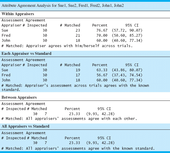

![]() FIGURE 8.17 Confidence intervals for the attribute agreement analysis.
FIGURE 8.17 Confidence intervals for the attribute agreement analysis.
8.7.6 Comparing Customer and Supplier Measurement Systems
In customer–supplier relationships it is often very important for the two parties to be able to reliably determine that the supplier’s product is within customer specifications. For the supplier, its internal measurement systems are essential to effective process control and/or final test and shipment. The customer must be able to verify the supplier’s claims regarding product quality. An essential component of the business relationship is the conformance of the two measurement systems. If the customer and supplier measurement systems are not in agreement, then differences in opinion about product quality can occur and the decision to accept or reject a shipment may become a basis for dispute between the two parties. This endangers the business relationship.
In many supply chains, it is common practice to compare the supplier and customer measurements of a given quantitative product characteristic in a shipment of product using a linear regression analysis technique. The general procedure is as follows. Suppose that the shipment consists of n units of product. The supplier measurements of the n units, say y1, y2 …, yn, are regressed on the corresponding n customer measurements, x1,x2, …, xn (or vice versa), and then the usual R2 statistic is computed. This is interpreted as the percentage of variation in the supplier’s measurements that is explained by the variation in the customer’s measurement. It is used as a measure of the degree of conformance between the two measurement systems. Frequently, a rule of thumb is that if the value of R2 is less than some arbitrary value (say 80%), it is concluded that the two measurement systems are not in conformance. Nachtsheim and Becker (2011) show that the R2 statistic is never an appropriate statistic for making this decision. They demonstrate that the R2 statistic can be arbitrarily small, even when the two measurement systems are in complete conformance. They provide an example in which by changing the capability of the supplier’s production process, the R2 statistic will change from 19% to 98% even though the two measurement systems are exactly the same (and therefore in complete conformance).
Nachtsheim and Becker (2011) show through a series of examples that:
1. The value of R2 depends directly on the standard deviation of the distribution of the true product characteristics, the standard deviation of the supplier’s measurement error distribution, and the standard deviation of the customer’s measurement error distribution.
2. As the standard deviation of the supplier’s product quality characteristic approaches zero, the value of R2 will approach the squared correlation between the supplier and customer measurement errors. This means that if the supplier’s process distribution is very tightly controlled (which is a good thing), R2 will approach the squared correlation between the supplier and customer errors—which will generally be near zero. So if a supplier’s process standard deviation is small (relative to the measurement error distributions), the use of R2 as a guide to performance of the two measurement systems will often lead to the erroneous conclusion that the measurement systems are not in conformity.
3. As the standard deviation of the supplier’s product quality characteristic approaches infinity (becomes very large, indicating a poorly controlled process with lots of variability), the value of R2 will approach unity. So if the supplier’s process distribution is not tightly controlled, one may conclude that the two measurement systems are in conformance.
4. As either measurement error standard deviation increases (relative to the process distribution), the value of R2 decreases.
5. As both measurement error standard deviations approach zero, the value of R2 will approach unity.
Nachtsheim and Becker (2011) suggest that an appropriate approach for comparing measurement systems can be based on one described by Hawkins (2002). The procedure they recommend is as follows. Assume as we did previously that the n customer measurements are x1, x2, …, xn and the corresponding n supplier measurements are y1, y2, …, yn. Then
1. Compute the n sums and n differences:
Si = yi + xi, i = 1, 2, …, n
Di = yi − xi, i = 1, 2, …, n
2. Plot the values of Di on the y-axis versus the values of Si on the x axis. When the two measurement systems are in conformance, this plot will be similar to the standard plot of residuals against predicted values in a regression problem where the basic assumptions are met—that is, constant error variance, no outliers, no evidence of curvature, and no slope. If this is the case, conformity of the measurement systems can be determined by using a paired t-test of the hypothesis H0: μD = 0; that is, the mean of the differences is zero. If the differences are not approximately normally distributed, either transformations or the sign test could be used instead of the t-test. Linear regression methods can be used to check for each type of non-conformity and are described in the next steps.
3. Check for non-constant variance. If the variances of x and y are constant, the vertical range of the differences will be approximately constant for all values of the sum. If this is not the case, then unequal variance is indicated for at least one of the measurements. A right-opening megaphone shape is frequently an indication that the variance of the differences is increasing with the sum of the measurements.
4. Check for outliers. This is indicated by a large vertical deviation on the plot.
5. Check for linear trend: Regress the values of Di versus the values of Si and test for a zero slope. If the slope is significantly different than zero, this suggests that the slope between y and x is not equal to unity, so there is a relative bias between the two measurement systems. The presence of bias would need to be resolved through linear calibration.
6. Check for curvature. The presence of curvature can usually be assessed visually. The presence of curvature implies bias that can only be resolved through nonlinear calibration.
8.8 Setting Specification Limits on Discrete Components
It is often necessary to use information from a process capability study to set specifications on discrete parts or components that interact with other components to form the final product. This is particularly important in complex assemblies to prevent tolerance stack-up problems where there are many interacting dimensions. This section discusses some aspects of setting specifications on components to ensure that the final product meets specifications. Some of these concepts are an integral part of design for Six Sigma (DFSS).
8.8.1 Linear Combinations
In many cases, the dimension of an item is a linear combination of the dimensions of the component parts. That is, if the dimensions of the components are x1, x2, …, xn, then the dimension of the final assembly is
where the ac are constants.
If the xi are normally and independently distributed with mean μi and variance ![]() , then y is normally distributed with mean
, then y is normally distributed with mean ![]() and variance
and variance ![]() . Therefore, if μi and
. Therefore, if μi and ![]() are known for each component, the fraction of assembled items falling outside the specifications can be determined.
are known for each component, the fraction of assembled items falling outside the specifications can be determined.
EXAMPLE 8.8 Meeting Customer Specifications
A linkage consists of four components as shown in Figure 8.18. The lengths of x1, x2, x3, and x4 are known to be x1 ∼ N(2.0, 0.0004), x2 ∼ N(4.5, 0.0009), x3 ∼ N(3.0, 0.0004), and x4 ∼ N(2.5, 0.0001). The lengths of the components can be assumed independent, because they are produced on different machines. All lengths are in inches. Determine the proportion of linkages that meet the customer specification on overall length of 12 ± 0.10.
To find the fraction of linkages that fall within design specification limits, note that y is normally distributed with mean
µy = 2.0 + 4.5 + 3.0 +2.5 = 12.0
and variance
![]()

![]() FIGURE 8.18 A linkage assembly with four components.
FIGURE 8.18 A linkage assembly with four components.
To find the fraction of linkages that are within specification, we must evaluate
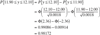
Therefore, we conclude that 98.172% of the assembled linkages will fall within the specification limits. This is not a Six Sigma product.
Sometimes it is necessary to determine specification limits on the individual components of an assembly so that specification limits on the final assembly will be satisfied. This is demonstrated in Example 8.9.
EXAMPLE 8.9 Designing a Six Sigma Product
Consider the assembly shown in Figure 8.19. Suppose that the specifications on this assembly are 6.00 ± 0.06 in. Let each component x1, x2, and x3 be normally and independently distributed with means µ1 = 1.00 in., µ2 = 3.00 in., and µ3 = 2.00 in., respectively. Suppose that we want the specification limits to fall inside the natural tolerance limits of the process for the final assembly so that Cp = 2.0, approximately, for the final assembly. This is a Six Sigma product, resulting in about 3.4 defective assemblies per million.
The length of the final assembly is normally distributed. Furthermore, if as a Six Sigma product, this implies that the natural tolerance limits must be located at µ ± 6σy. Now µy = µ1 + µ2 + µ3 = 1.00 + 3.00 + 2.00 = 6.00, so the process is centered at the nominal value. Therefore, the maximum possible value of σy that would yield an acceptable product is
![]()
That is, if σy ≤ 0.010, then the number of nonconforming assemblies produced will be acceptable.
Now let us see how this affects the specifications on the individual components. The variance of the length of the final assembly is
![]()
Suppose that the variances of the component lengths are all equal—that is, ![]() (say). Then
(say). Then
![]()
and the maximum possible value for the variance of the length of any component is
![]()
Effectively, if σ2 ≤ 0.000033 for each component, then the natural tolerance limits for the final assembly will be inside the specification limits such that Cp = 2.0.
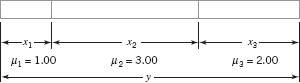
![]() Figure 8.19 Assembly for Example 8.9.
Figure 8.19 Assembly for Example 8.9.
This can be translated into specification limits on the individual components. If we assume that the natural tolerance limits and the specification limits for the components are to coincide exactly, then the specification limits for each component are as follows:

It is possible to give a general solution to the problem in Example 8.9. Let the assembly consist of n components having common variance σ2. If the natural tolerances of the assembly are defined so that no more than α% of the assemblies will fall outside these limits, and 2W is the width of the specification limits, then
is the maximum possible value for the variance of the final assembly that will permit the natural tolerance limits and the specification limits to coincide. Consequently, the maximum permissible value of the variance for the individual components is
EXAMPLE 8.10 Assembly of a Shaft and a Bearing
A shaft is to be assembled into a bearing. The internal diameter of the bearing is a normal random variable—say, x1—with mean µ1 = 1.500 in. and standard deviation σ1 = 0.0020 in. The external diameter of the shaft—say, x2—is normally distributed with mean µ2 = 1.480 in. and standard deviation σ2 = 0.0040 in. The assembly is shown in Figure 8.20.
When the two parts are assembled, interference will occur if the shaft diameter is larger than the bearing diameter—that is, if
y = x1 − x2 < 0
Note that the distribution of y is normal with mean
µy = µ − µ = 1.500 − 1.480 =0.020
and variance
![]()
Therefore, the probability of interference is
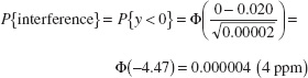
which indicates that very few assemblies will have interference. This is essentially a Six Sigma design.
In problems of this type, we occasionally define a minimum clearance—say, C—such that
P{clearance < C} = α
Thus, C becomes the natural tolerance for the assembly and can be compared with the design specification. In our example, if we establish α = 0.0001 (i.e., only 1 out of 10,000 assemblies or 100 ppm will have clearance less than or equal to C), then we have
![]()

![]() Figure 8.20 Assembly of a shaft and a bearing.
Figure 8.20 Assembly of a shaft and a bearing.
![]()
which implies that ![]() . That is, only 1 out of 10,000 assemblies will have clearance less than 0.0034 in.
. That is, only 1 out of 10,000 assemblies will have clearance less than 0.0034 in.
8.8.2 Nonlinear Combinations
In some problems, the dimension of interest may be a nonlinear function of the n component dimensions x1, x2,. .. xn—say,
In problems of this type, the usual approach is to approximate the nonlinear function g by a linear function of the xi in the region of interest. If µ1, µ2,. .. µn are the nominal dimensions associated with the components x1, x2,. .. xn, then by expanding the right-hand side of equation 8.41 in a Taylor series about µ1, µ2,. .. µn, we obtain
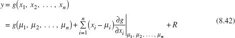
where R represents the higher-order terms. Neglecting the terms of higher order, we can apply the expected value and variance operators to obtain
and
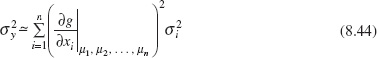
This procedure to find an approximate mean and variance of a nonlinear combination of random variables is sometimes called the delta method. Equation 8.44 is often called the transmission of error formula.
The following example illustrates how these results are useful in tolerance problems.
EXAMPLE 8.11 A Product with Nonlinear Dimensions
Consider the simple DC circuit components shown in Figure 8.21. Suppose that the voltage across the points (a, b) is required to be 100 ± 2 V. The specifications on the current and the resistance in the circuit are shown in Figure 8.21. We assume that the component random variables I and R are normally and independently distributed with means equal to their nominal values.
From Ohm’s law, we know that the voltage is
V = IR

![]() Figure 8.21
Figure 8.21
Electrical circuit for
Example 8.11.
Since this involves a nonlinear combination, we expand V in a Taylor series about mean current µI and mean resistance µR, yielding
V ≃ µI µR + (I − µI)µR + (R − µR) µI
neglecting the terms of higher order. Now the mean and variance of voltage are
µV ≃ µIµR
and
![]()
approximately, where ![]() and
and ![]() are the variances of I and R, respectively.
are the variances of I and R, respectively.
Now suppose that I and R are centered at their nominal values and that the natural tolerance limits are defined so that α = 0.0027 is the fraction of values of each component falling outside these limits. Assume also that the specification limits are exactly equal to the natural tolerance limits. For the current I we have I = 25 ± 1 A. That is, 24 ≤ I ≤ 26 A correspond to the natural tolerance limits and the specifications. Since I ~ N(25, ![]() ), and since Zα/2 = Z0.00135 = 3.00, we have
), and since Zα/2 = Z0.00135 = 3.00, we have
![]()
or σI = 0.33. For the resistance, we have R = 4 ± 0.06 ohm as the specification limits and the natural tolerance limits. Thus,
![]()
and σR = 0.02. Note that σI and σR are the largest possible values of the component standard deviations consistent with the natural tolerance limits falling inside or equal to the specification limits.
Using these results, and if we assume that the voltage V is approximately normally distributed, then
µV ≃ µIµR = (25)(4) = 100 V
and
![]()
approximately. Thus ![]() . Therefore, the probability that the voltage will fall within the design specifications is
. Therefore, the probability that the voltage will fall within the design specifications is
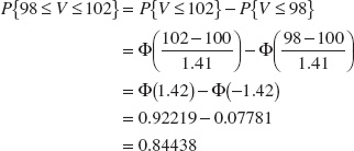
That is, only 84% of the observed output voltages will fall within the design specifications. Note that the natural tolerance limits or process capability for the output voltage is
µV ± 3.00σV
or
100 ± 4.23 V
In this problem the process capability ratio is
![]()
Note that, although the individual current and resistance variations are not excessive relative to their specifications, because of tolerance stack-up problems, they interact to produce a circuit whose performance relative to the voltage specifications is very poor.
8.9 Estimating the Natural Tolerance Limits of a Process
In many types of production processes, it is customary to think of the natural tolerance limits as those limits that contain a certain fraction—say, 1 − α—of the distribution. In this section we present some approaches to estimating the natural tolerance limits of a process.
If the underlying distribution of the quality characteristic and its parameters are known—say, on the basis of long experience—then the tolerance limits may be readily established. For example, in Section 8.7, we studied several problems involving tolerances where the quality characteristic was normally distributed with known mean µ and known variance σ2. If in this case we define the tolerance limits as those limits that contain 100(1 − α)% of the distribution of this quality characteristic, then these limits are simply µ ± Zα/2σ. If α = 0.05 (say), then the tolerance limits are given by µ ± 1.96σ.
In most practical problems, both the form of the distribution and its parameters will be unknown. However, the parameters may usually be estimated from sample data. In certain cases, then, it is possible to estimate the tolerance limits of the process by use of these sample statistics. We will discuss two procedures for estimating natural tolerance limits, one for those situations in which the normality assumption is reasonable, and a nonparametric approach useful in cases where the normality assumption is inappropriate.
The estimation of the natural tolerance limits of a process is an important problem with many significant practical implications. As noted previously, unless the product specifications exactly coincide with or exceed the natural tolerance limits of the process (PCR ≥ 1), an extremely high percentage of the production will be outside specifications, resulting in a high loss or rework rate.
8.9.1 Tolerance Limits Based on the Normal Distribution
Suppose a random variable x is normally distributed with mean µ and variance σ2, both unknown. From a random sample of n observations, the sample mean ![]() and sample variance s2 may be computed. A logical procedure for estimating the natural tolerance limits µ ± Zα/2σ is to replace µ by
and sample variance s2 may be computed. A logical procedure for estimating the natural tolerance limits µ ± Zα/2σ is to replace µ by ![]() and σ by s, yielding
and σ by s, yielding

Since ![]() and s are only estimates and not the true parameter values, we cannot say that the above interval always contains 100(1 - α)% of the distribution. However, one may determine a constant K, such that in a large number of samples a fraction γ of the intervals
and s are only estimates and not the true parameter values, we cannot say that the above interval always contains 100(1 - α)% of the distribution. However, one may determine a constant K, such that in a large number of samples a fraction γ of the intervals ![]() ± Ks will include at least 100(1 – α)% of the distribution. Values of K for 2 ≤ n ≤ 1000, γ = 0.90, 0.95, 0.99, and α = 0.10, 0.05, and 0.01 are given in Appendix Table VII.
± Ks will include at least 100(1 – α)% of the distribution. Values of K for 2 ≤ n ≤ 1000, γ = 0.90, 0.95, 0.99, and α = 0.10, 0.05, and 0.01 are given in Appendix Table VII.
EXAMPLE 8.12Constructing a Tolerance Interval
The manufacturer of a solid-fuel rocket propellant is interested in finding the tolerance limits of the process such that 95% of the burning rates will lie within these limits with probability 0.99. It is known from previous experience that the burning rate is normally distributed. A random sample of 25 observations shows that the sample mean and variance of burning rate are ![]() = 40.75 and s2 = 1.87, respectively. Since α = 0.05, γ = 0.99, and n = 25, we find K = 2.972 from Appendix Table VII. Therefore, the required tolerance limits are found as
= 40.75 and s2 = 1.87, respectively. Since α = 0.05, γ = 0.99, and n = 25, we find K = 2.972 from Appendix Table VII. Therefore, the required tolerance limits are found as ![]() ± 2.972s = 40.75 ± (2.972)(1.37) = 40.75 ± 4.07 = [36.68, 44.82].
± 2.972s = 40.75 ± (2.972)(1.37) = 40.75 ± 4.07 = [36.68, 44.82].
We note that there is a fundamental difference between confidence limits and tolerance limits. Confidence limits are used to provide an interval estimate of the parameter of a distribution, whereas tolerance limits are used to indicate the limits between which we can expect to find a specified proportion of a population. Note that as n approaches infinity, the length of a confidence interval approaches zero, while the tolerance limits approach the corresponding value for the population. Thus, in Appendix Table VII, as n approaches infinity for α = 0.05, say, K approaches 1.96.
It is also possible to specify one-sided tolerance limits based on the normal distribution. That is, we may wish to state that with probability γ at least 100(1 – α)% of the distribution is greater than the lower tolerance limit ![]() – Ks or less than the upper tolerance limit
– Ks or less than the upper tolerance limit ![]() + Ks. Values of K for these one-sided tolerance limits for 2 ≤ n ≤ 1000, γ = 0.90, 0.95, 0.99, and α = 0.10, 0.05, and 0.01 are given in Appendix Table VIII.
+ Ks. Values of K for these one-sided tolerance limits for 2 ≤ n ≤ 1000, γ = 0.90, 0.95, 0.99, and α = 0.10, 0.05, and 0.01 are given in Appendix Table VIII.
8.9.2 Nonparametric Tolerance Limits
It is possible to construct nonparametric (or distribution-free) tolerance limits that are valid for any continuous probability distribution. These intervals are based on the distribution of the extreme values (largest and smallest sample observation) in a sample from an arbitrary continuous distribution. For two-sided tolerance limits, the number of observations that must be taken to ensure that with probability γ at least 100(1 – α)% of the distribution will lie between the largest and smallest observations obtained in the sample is
![]()
approximately. Thus, to be 99% certain that at least 95% of the population will be included between the sample extreme values, we have α = 0.05, γ = 0.99, and consequently,
![]()
For one-sided nonparametric tolerance limits such that with probability γ at least 100(1 – α)% of the population exceeds the smallest sample value (or is less than the largest sample value), we must take a sample of
![]()
observations. Thus, the upper nonparametric tolerance limit that contains at least 90% of the population with probability at least 0.95 (α = 0.10 and γ = 0.95) is the largest observation in a sample of
![]()
observations.
In general, nonparametric tolerance limits have limited practical value, because to construct suitable intervals that contain a relatively large fraction of the distribution with high probability, large samples are required. In some cases, the sample sizes required may be so large as to prohibit their use. If one can specify the form of the distribution, it is possible for a given sample size to construct tolerance intervals that are narrower than those obtained from the nonparametric approach.
Important Terms and Concepts
ANOVA approach to a gauge R & R experiment
Components of gauge error
Components of measurement error
Confidence intervals for gauge R & R studies
Confidence intervals on process capability ratios
Consumer’s risk or missed fault for a gauge
Control charts and process capability analysis
Delta method
Discrimination ratio (DR) for a gauge
Estimating variance components
Factorial experiment
Gauge R & R experiment
Graphical methods for process capability analysis
Measurement systems capability analysis
Natural tolerance limits for a normal distribution
Natural tolerance limits of a process
Nonparametric tolerance limits
Normal distribution and process capability ratios
One-sided process-capability ratios
PCR Cp
PCR Cpk
PCR Cpm
Precision and accuracy of a gauge
Precision-to-tolerance (P/T) ratio
Process capability
Process capability analysis
Process performance indices Pp and Ppk
Producer’s risk or false failure for a gauge
Product characterization
Random effects model ANOVA
Signal-to-noise ratio (SNR) for a gauge
Tolerance stack-up problems
Transmission of error formula
Exercises
![]() The Student Resource Manual presents comprehensive annotated solutions to the odd-numbered exercises included in the Answers to Selected Exercises section in the back of this book.
The Student Resource Manual presents comprehensive annotated solutions to the odd-numbered exercises included in the Answers to Selected Exercises section in the back of this book.
8.1. A process is in statistical control with ![]() = 20 and s = 1.2. Specifications are at LSL = 16 and USL = 24.
= 20 and s = 1.2. Specifications are at LSL = 16 and USL = 24.
(a) Estimate the process capability with an appropriate process capability ratio.
(b) Items that are produced below the lower specification limit must be scrapped, while items that are above the upper specification limit can be reworked. What proportion of the process output is scrap, and what proportion is rework?
(c) Suppose that scrap is four times as expensive as rework. Does this suggest that moving the process center could reduce overall costs? What value of the process target would you recommend?
8.2. A process is in statistical control with ![]() = 202.5 and s = 2.0. Specifications are at LSL = 196 and USL = 206.
= 202.5 and s = 2.0. Specifications are at LSL = 196 and USL = 206.
(a) Estimate the process capability with an appropriate process capability ratio.
(b) What is the potential capability of this process?
(c) Items that are produced below the lower specification limit must be scrapped, while items that are above the upper specification limit can be reworked. What proportion of the process output is scrap and what proportion is rework?
(d) Because scrap is more expensive than rework, the process has been centered closer to the upper specification limit. If scrap is twice as expensive as rework, is the process mean at the best possible location? What value of the process target would you recommend?
8.3. Consider the piston ring data in Table 6.3. Estimate the process capability assuming that specifications are 74.00 ± 0.035 mm.
8.4. Perform a process capability analysis using ![]() and R charts for the data in Exercise 6.7.
and R charts for the data in Exercise 6.7.
8.5. Estimate process capability using ![]() and R charts for the power supply voltage data in Exercise 6.8. If specifications are at 350 ± 5 V, calculate Cp, Cpk, and Cpkm. Interpret these capability ratios.
and R charts for the power supply voltage data in Exercise 6.8. If specifications are at 350 ± 5 V, calculate Cp, Cpk, and Cpkm. Interpret these capability ratios.
8.6. Consider the hole diameter data in Exercise 6.9. Estimate process capability using ![]() and R charts. If specifications are at 0 ± 0.01, calculate Cp, Cpk, and Cpkm. Interpret these ratios.
and R charts. If specifications are at 0 ± 0.01, calculate Cp, Cpk, and Cpkm. Interpret these ratios.
8.7. A process is in control with ![]() = 100,
= 100, ![]() = 1.05, and n = 5. The process specifications are at 95 ± 10. The quality characteristic has a normal distribution.
= 1.05, and n = 5. The process specifications are at 95 ± 10. The quality characteristic has a normal distribution.
(a) Estimate the potential capability.
(b) Estimate the actual capability.
(c) How much could the fallout in the process be reduced if the process were corrected to operate at the nominal specification?
8.8. A process is in statistical control with ![]() = 199 and
= 199 and ![]() = 3.5. The control chart uses a sample size of n = 4. Specifications are at 200 ± 8. The quality characteristic is normally distributed.
= 3.5. The control chart uses a sample size of n = 4. Specifications are at 200 ± 8. The quality characteristic is normally distributed.
(a) Estimate the potential capability of the process.
(b) Estimate the actual process capability.
(c) How much improvement could be made in process performance if the mean could be centered at the nominal value?
8.9. A process is in statistical control with ![]() = 39.7 and
= 39.7 and ![]() = 2.5. The control chart uses a sample size of n = 2. Specifications are at 40 ± 5. The quality characteristic is normally distributed.
= 2.5. The control chart uses a sample size of n = 2. Specifications are at 40 ± 5. The quality characteristic is normally distributed.
(a) Estimate the potential capability of the process.
(b) Estimate the actual process capability.
(c) Calculate and compare the PCRs Cpkm and Cpkm.
(d) How much improvement could be made in process performance if the mean could be centered at the nominal value?
8.10. A process is in control with ![]() = 75 and
= 75 and ![]() = 2. The process specifications are at 80 ± 8. The sample size n = 5.
= 2. The process specifications are at 80 ± 8. The sample size n = 5.
(a) Estimate the potential capability.
(b) Estimate the actual capability.
(c) How much could process fallout be reduced by shifting the mean to the nominal dimension? Assume that the quality characteristic is normally distributed.
8.11. Consider the two processes shown in Table 8E.1 (the sample size n = 5):![]() Table 8E.1
Table 8E.1
Process Data for Exercise 8.11
Specifications are at 100 ± 10. Calculate Cp, Cpk, and Cpm and interpret these ratios. Which process would you prefer to use?
8.12. Suppose that 20 of the parts manufactured by the processes in Exercise 8.11 were assembled so that their dimensions were additive; that is,
x = x1 + x2 +. .. + x20
Specifications on x are 2,000 ± 200. Would you prefer to produce the parts using process A or process B? Why? Do the capability ratios computed in Exercise 8.11 provide any guidance for process selection?
8.13. The weights of nominal 1-kg containers of a concentrated chemical ingredient are shown in Table 8E.2. Prepare a normal probability plot of the data and estimate process capability. Does this conclusion depend on process stability?
8.14. Consider the package weight data in Exercise 8.13. Suppose there is a lower specification at 0.985 kg. Calculate an appropriate process capability ratio for this material. What percentage of the packages
![]() Table 8E.2
Table 8E.2
Weights of Containers
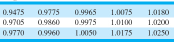
![]() Table 8E.3
Table 8E.3
Cycle Time Data for Exercise 8.15
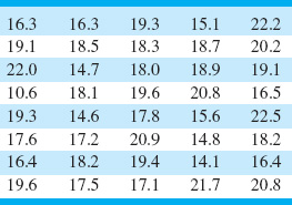
produced by this process is estimated to be below the specification limit?
8.15. Table 8E.3 presents data on the cycle time (in hours) to process small loan applications. Prepare a normal probability plot of these data. The loan agency has a promised decision time to potential customers of 24 hours. Based on the data in the table and the normal probability plot, what proportion of the customers will experience longer waiting times?
8.16. Table 8E.4 presents data on the waiting time (in minutes) to see a nurse or physician in a hospital emergency department. The hospital has a policy of seeing all patients initially within ten minutes of arrival.
(a) Prepare a normal probability plot of these data. Does the normal distribution seem to be an appropriate model for these data?
(b) Prepare a normal probability plot of the natural logarithm of these data. Does the normal distribution seem to be an appropriate model for the transformed data?
(c) Based on the data in Table 8E.4 and the normal probability plots, what proportion of the patients will not see a nurse or physician within ten minutes of arrival?
8.17. The height of the disk used in a computer disk drive assembly is a critical quality characteristic. Table 8E.5 gives the heights (in mm) of 25 disks randomly
![]() Table 8E.4
Table 8E.4
Waiting Time Data for Exercise 8.16

![]() Table 8E.5
Table 8E.5
Disk Height Data for Exercise 8.17
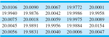
selected from the manufacturing process. Assume that the process is in statistical control. Prepare a normal probability plot of the disk height data and estimate process capability.
8.18. The length of time required to reimburse employee expense claims is a characteristic that can be used to describe the performance of the process. Table 8E.6 gives the cycle times (in days) of 30 randomly selected employee expense claims. Estimate the capability of this process. Do your conclusions depend on statistical control of the process?
8.19. An electric utility tracks the response time to customer-reported outages. The data in Table 8E.7 are a random sample of 40 of the response times (in minutes) for one operating division of this utility during a single month.
(a) Estimate the capability of the utility’s process for responding to customer-reported outages.
(b) The utility wants to achieve a 90% response rate in under two hours, as response to emergency outages is an important measure of customer satisfaction. What is the capability of the process with respect to this objective?
8.20. Consider the hardness data in Exercise 6.62. Use a probability plot to assess normality. Estimate process capability.
8.21. The failure time in hours of ten LSI memory devices follows: 1210, 1275, 1400, 1695, 1900, 2105, 2230,
![]() Table 8E.6
Table 8E.6
Days to Par Expense Claims

![]() Table 8E.7
Table 8E.7
Response Time Data for Exercise 8.19
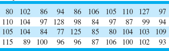
2250, 2500, and 2625. Plot the data on normal probability paper and, if appropriate, estimate process capability. Is it safe to estimate the proportion of circuits that fail below 1,200 h?
8.22. A normally distributed process has specifications of LSL = 75 and USL = 85 on the output. A random sample of 25 parts indicates that the process is centered at the middle of the specification band, and the standard deviation is s = 1.5.
(a) Find a point estimate of Cp.
(b) Find a 95% confidence interval on Cp. Comment on the width of this interval.
8.23. A company has been asked by an important customer to demonstrate that its process capability ratio Cp exceeds 1.33. It has taken a sample of 50 parts and obtained the point estimate ![]() = 1.52. Assume that the quality characteristic follows a normal distribution. Can the company demonstrate that Cp exceeds 1.33 at the 95% level of confidence? What level of confidence would give a one-sided lower confidence limit on Cp that exceeds 1.33?
= 1.52. Assume that the quality characteristic follows a normal distribution. Can the company demonstrate that Cp exceeds 1.33 at the 95% level of confidence? What level of confidence would give a one-sided lower confidence limit on Cp that exceeds 1.33?
8.24. Suppose that a quality characteristic has a normal distribution with specification limits at USL = 100 and LSL = 90. A random sample of 30 parts results in ![]() = 97 and s = 1.6.
= 97 and s = 1.6.
(a) Calculate a point estimate of Cpk.
(b) Find a 95% confidence interval on Cpk.
8.25. The molecular weight of a particular polymer should fall between 2,100 and 2,350. Fifty samples of this material were analyzed with the results
![]() = 2,275 and s = 60. Assume that molecular weight is normally distributed.
= 2,275 and s = 60. Assume that molecular weight is normally distributed.
(a) Calculate a point estimate of Cpk.
(b) Find a 95% confidence interval on Cpk.
8.26. A normally distributed quality characteristic has specification limits at LSL = 10 and USL = 20. A random sample of size 50 results in ![]() = 16 and s = 12.
= 16 and s = 12.
(a) Calculate a point estimate of Cpk.
(b) Find a 95% confidence interval on Cpk.
8.27. A normally distributed quality characteristic has specification limits at LSL = 50 and USL = 60. A random sample of size 35 results in ![]() = 55.5 and s = 0.9.
= 55.5 and s = 0.9.
(a) Calculate a point estimate of Cpk.
(b) Find a 95% confidence interval on Cpk.
(c) Is this a 6σ-process?
8.28. Consider a simplified version of equation 8.19:
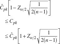
Note that this was obtained by assuming that the term 9n in equation 8.19 will probably be large. Rework Exercise 8.24 using this equation and compare your answer to the original answer obtained from equation 8.19. How good is the approximation suggested in this problem?
8.29. An operator–instrument combination is known to test parts with an average error of zero; however, the standard deviation of measurement error is estimated to be 3. Samples from a controlled process were analyzed, and the total variability was estimated to be ![]() = 5. What is the true process standard deviation?
= 5. What is the true process standard deviation?
8.30. Consider the situation in Example 8.7. A new gauge is being evaluated for this process. The same operator measures the same 20 parts twice using the new gauge and obtains the data shown in Table 8E.8.
(a) What can you say about the performance of the new gauge relative to the old one?
(b) If specifications are at 25 ± 15, what is the P/T ratio for the new gauge?
8.31. Ten parts are measured three times by the same operator in a gauge capability study. The data are shown in Table 8E.9.
(a) Describe the measurement error that results from the use of this gauge.
(b) Estimate total variability and product variability.
(c) What percentage of total variability is due to the gauge?
(d) If specifications on the part are at 100 ± 15, find the P/T ratio for this gauge. Comment on the adequacy of the gauge.
8.32. In a study to isolate both gauge repeatability and gauge reproducibility, two operators use the same
![]() Table 8E.8
Table 8E.8
Measurement Data for Exercise 8.30

![]() Table 8E.9
Table 8E.9
Measurement Data for Exercise 8.31
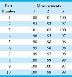
gauge to measure ten parts three times each. The data are shown in Table 8E.10.
(a) Estimate gauge repeatability and reproducibility.
(b) Estimate the standard deviation of measurement error.
(c) If the specifications are at 50 ± 10, what can you say about gauge capability?
8.33. The data in Table 8E.11 were taken by one operator during a gauge capability study.
(a) Estimate gauge capability.
(b) Does the control chart analysis of these data indicate any potential problem in using the gauge?
![]() Table 8E.10
Table 8E.10
Measurement Data for Exercise 8.32
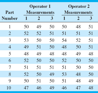
![]() Table 8E.11
Table 8E.11
Measurement Data for Exercise 8.33

8.34. A measurement systems experiment involving 20 parts, three operators, and two measurements per part is shown in Table 8E.12.
(a) Estimate the repeatability and reproducibility of the gauge.
(b) What is the estimate of total gauge variability?
(c) If the product specifications are at LSL = 6 and USL = 60, what can you say about gauge capability?
![]() Table 8E.12
Table 8E.12
Measurement Data for Exercise 8.34
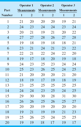
8.35. Reconsider the gauge R & R experiment in Exercise 8.34. Calculate the quantities SNR and DR for this gauge. Discuss what information these measures provide about the capability of the gauge.
8.36. Three parts are assembled in series so that their critical dimensions x1, x2,and x3 add. The dimensions of each part are normally distributed with the following parameters: µ1 = 100, σ1 = 4, µ2 = 75, σ2 = 4, µ3 = 75, and σ3 = 2. What is the probability that an assembly chosen at random will have a combined dimension in excess of 262?
8.37. Two parts are assembled as shown in the figure. The distributions of x1 and x2 are normal, with µ1 = 20, σ1 = 0.3, µ2 = 19.6, and σ2 = 0.4. The specifications of the clearance between the mating parts are 0.5 ± 0.4. What fraction of assemblies will fail to meet specifications if assembly is at random?

8.38. A product is packaged by filling a container completely full. This container is shaped as shown in the figure. The process that produces these containers is examined, and the following information collected on the three critical dimensions:

Assuming the variables to be independent, what are approximate values for the mean and variance of container volume?
8.39. A rectangular piece of metal of width W and length L is cut from a plate of thickness T. If W, L, and T are independent random variables with means and standard deviations as given here and the density of the metal is 0.08 g/cm3, what would be the estimated mean and standard deviation of the weights of pieces produced by this process?
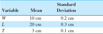
8.40. The surface tension of a chemical product, measured on a coded scale, is given by the relationship
s = (3 + 0.05x)2
where x is a component of the product with probability distribution
![]()
Find the mean and variance of s.
8.41. Two resistors are connected to a battery as shown in the figure. Find approximate expressions for the mean and variance of the resulting current (I). E, R1, and R2 are random variables with means µE, µR1, µR2, and variances ![]() , respectively.
, respectively.
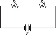
8.42. Two mating parts have critical dimensions x1 and x2 as shown in the figure. Assume that x1 and x2 are normally distributed with means µ1 and µ2 and standard deviations σ1 = 0.400 and σ2 = 0.300. If it is desired that the probability of a smaller clearance (i.e., x1 − x2) than 0.09 should be 0.006, what distance between the average dimension of the two parts (i.e., µ1 − µ2) should be specified by the designer?
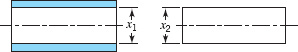
8.43. An assembly of two parts is formed by fitting a shaft into a bearing. It is known that the inside diameters of bearings are normally distributed with mean 2.010 cm and standard deviation 0.002 cm, and that the outside diameters of the shafts are normally distributed with mean 2.004 cm and standard deviation 0.001 cm. Determine the distribution of clearance between the parts if random assembly is used. What is the probability that the clearance is positive?
8.44. We wish to estimate a two-sided natural tolerance interval that will include 99% of the values of a random variable with probability 0.80. If nothing is known about the distribution of the random variable, how large should the sample be?
8.45. A sample of ten items from a normal population had a mean of 300 and a standard deviation of 10. Using these data, estimate a value for the random variable such that the probability is 0.95 that 90% of the measurements on this random variable will lie below the value.
8.46. A sample of 25 measurements on a normally distributed quality characteristic has a mean of 85 and a standard deviation of 1. Using a confidence probability of 0.95, find a value such that 90% of the future measurements on this quality characteristic will lie above it.
8.47. A sample of 20 measurements on a normally distributed quality characteristic had ![]() = 350 and s = 10. Find an upper natural tolerance limit that has probability 0.90 of containing 95% of the distribution of this quality characteristic.
= 350 and s = 10. Find an upper natural tolerance limit that has probability 0.90 of containing 95% of the distribution of this quality characteristic.
8.48. How large a sample is required to obtain a natural tolerance interval that has probability 0.90 of containing 95% of the distribution? After the data are collected, how would you construct the interval?
8.49. A random sample of n = 40 pipe sections resulted in a mean wall thickness of 0.1264 in. and a standard deviation of 0.0003 in. We assume that wall thickness is normally distributed.
(a) Between what limits can we say with 95% confidence that 95% of the wall thicknesses should fall?
(b) Construct a 95% confidence interval on the true mean thickness. Explain the difference between this interval and the one constructed in part (a).
8.50. Find the sample size required to construct an upper nonparametric tolerance limit that contains at least 95% of the population with probability at least 0.95. How would this limit actually be computed from sample data?
_____________________________
1The experimental structure here is that of a factorial design. See Chapter 13 and the supplemental text material for more details about the analysis of variance, including computing.