
14Process Optimization with Designed Experiments
CHAPTER OUTLINE
14.1 RESPONSE SURFACE METHODS AND DESIGNS
14.1.1 The Method of Steepest Ascent
14.1.2 Analysis of a Second-Order Response Surface
14.2 PROCESS ROBUSTNESS STUDIES
14.2.2 The Response Surface Approach to Process Robustness Studies
Supplemental Material for Chapter 14
S14.1 Response Surface Designs
S14.2 More about Robust Design and Process Robustness Studies
The supplemental material is on the textbook Website www.wiley.com/college/montgomery.
CHAPTER OVERVIEW AND LEARNING OBJECTIVES
In Chapter 13, we focused on factorial and fractional factorial designs. These designs are very useful for factor screening—that is, identifying the most important factors that affect the performance of a process. Sometimes this is called process characterization. Once the appropriate subset of process variables is identified, the next step is usually process optimization, or finding the set of operating conditions for the process variables that result in the best process performance. This chapter gives a brief account of how designed experiments can be used in process optimization.
We discuss and illustrate response surface methodology, an approach to optimization developed in the early 1950s and initially applied in the chemical and process industries. This is probably the most widely used and successful optimization technique based on designed experiments. Then we discuss how designed experiments can be used in process robustness studies. These are activities in which process engineering personnel try to reduce the variability in the output of a process by setting controllable factors to levels that minimize the variability transmitted into the responses of interest by other factors that are difficult to control during routine operation. We also present an example of evolutionary operation, an approach to maintaining optimum performance that is, in effect, an on-line or in-process application of the factorial design concepts of Chapter 13.
After careful study of this chapter, you should be able to do the following:
- Know how to use the response surface approach to optimizing processes
- Know how to apply the method of steepest ascent
- Know how to analyze a second-order response surface model
- Know how to determine optimum operating conditions for a process
- Know how to set up and conduct an experiment using a central composite design
- Understand the difference between controllable process variables and noise variables
- Understand the advantages of a combined array design for a process robustness study
- Know how to use the response model approach to conduct a process robustness study
- Know how evolutionary operation (EVOP) is used to maintain a process that is subject to drift near its optimum operating conditions
14.1 Response Surface Methods and Designs
Response surface methodology (RSM) is a collection of mathematical and statistical techniques that are useful for modeling and analysis in applications where a response of interest is influenced by several variables and the objective is to optimize this response. The general RSM approach was developed in the early 1950s and was initially applied in the chemical industry with considerable success. Over the past 20 years RSM has found extensive application in a wide variety of industrial settings, far beyond its origins in chemical processes, including semiconductor and electronics manufacturing, machining, metal cutting, and joining processes, among many others. Many statistics software packages have included the experimental designs and optimization techniques that make up the basics of RSM as standard features. For a recent comprehensive presentation of RSM, see Myers, Montgomery, and Anderson-Cook (2009).
To illustrate the general idea of RSM, suppose that a chemical engineer wishes to find the levels of reaction temperature (x1) and reaction time (x2) that maximize the yield (y) of a process. The process yield is a function of the levels of temperature and time—say,
y = f (x1, x2) + ε
where ε represents the noise or error observed in the response y. If we denote the expected value of the response by E(y) = f (x1, x2), then the surface represented by
E(y) = f (x1, x2)
is called a response surface. Recall that we introduced the idea of a response surface in Chapter 13, where we presented an example of a response surface generated from a model that arose from a factorial design.
We may represent the response surface graphically as shown in Figure 14.1, where E(y) is plotted versus the levels of x1 and x2. Note that the response is represented as a surface plot in three-dimensional space. To help visualize the shape of a response surface, we often plot the contours of the response surface as shown in Figure 14.2. In the contour plot, lines of constant response are drawn in the x1, x2 plane. Each contour corresponds to a particular height of the response surface. The contour plot is helpful in studying the levels of x1, x2 that result in changes in the shape or height of the response surface.
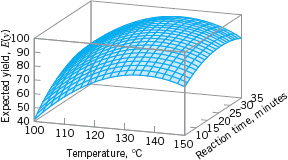
![]() FIGURE 14.1 A three-dimensional response surface showing the expected yield as a function of reaction temperature and reaction time.
FIGURE 14.1 A three-dimensional response surface showing the expected yield as a function of reaction temperature and reaction time.
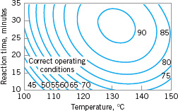
![]() FIGURE 14.2 A contour plot of the yield response surface in Figure 14.1.
FIGURE 14.2 A contour plot of the yield response surface in Figure 14.1.
In most RSM problems, the form of the relationship between the response and the independent variables is unknown. Thus, the first step in RSM is to find a suitable approximation for the true relationship between y and the independent variables. Usually, a low-order polynomial in some region of the independent variables is employed. If the response is well modeled by a linear function of the independent variables, then the approximating function is the first-order model

If there is curvature in the system, then a polynomial of higher degree must be used, such as the second-order model

Many RSM problems utilize one or both of these approximating polynomials. Of course, it is unlikely that a polynomial model will be a reasonable approximation of the true functional relationship over the entire space of the independent variables, but for a relatively small region they usually work quite well.
The method of least squares (see Chapter 4) is used to estimate the parameters in the approximating polynomials. That is, the estimates of the β’s in equations 14.1 and 14.2 are those values of the parameters that minimize the sum of squares of the model errors. The response surface analysis is then done in terms of the fitted surface. If the fitted surface is an adequate approximation of the true response function, then analysis of the fitted surface will be approximately equivalent to analysis of the actual system.
RSM is a sequential procedure. Often, when we are at a point on the response surface that is remote from the optimum, such as the current operating conditions in Figure 14.2, there is little curvature in the system and the first-order model will be appropriate. Our objective here is to lead the experimenter rapidly and efficiently to the general vicinity of the optimum. Once the region of the optimum has been found, a more elaborate model such as the second-order model may be employed, and an analysis may be performed to locate the optimum. From Figure 14.2, we see that the analysis of a response surface can be thought of as “climbing a hill,” where the top of the hill represents the point of maximum response. If the true optimum is a point of minimum response, then we may think of “descending into a valley.”
The eventual objective of RSM is to determine the optimum operating conditions for the system or to determine a region of the factor space in which operating specifications are satisfied. Also, note that the word “optimum” in RSM is used in a special sense. The “hill climbing” procedures of RSM guarantee convergence to a local optimum only.
14.1.1 The Method of Steepest Ascent
Frequently, the initial estimate of the optimum operating conditions for the system will be far away from the actual optimum. In such circumstances, the objective of the experimenter is to move rapidly to the general vicinity of the optimum. We wish to use a simple and economically efficient experimental procedure. When we are remote from the optimum, we usually assume that a first-order model is an adequate approximation to the true surface in a small region of the x’s.
The method of steepest ascent is a procedure for moving sequentially along the path of steepest ascent—that is, in the direction of the maximum increase in the response. Of course, if minimization is desired, then we would call this procedure the method of steepest descent. The fitted first-order model is
and the first-order response surface—that is, the contours of ŷ—is a series of parallel straight lines such as shown in Figure 14.3. The direction of steepest ascent is the direction in which ŷ increases most rapidly. This direction is normal to the fitted response surface contours. We usually take as the path of steepest ascent the line through the center of the region of interest and normal to the fitted surface contours. Thus, the steps along the path are proportional to the magnitudes of the regression coefficients ![]() . The experimenter determines the actual amount of movement along this path based on process knowledge or other practical considerations.
. The experimenter determines the actual amount of movement along this path based on process knowledge or other practical considerations.
Experiments are conducted along the path of steepest ascent until no further increase in response is observed or until the desired response region is reached. Then a new first-order model may be fitted, a new direction of steepest ascent determined, and, if necessary, further experiments conducted in that direction until the experimenter feels that the process is near the optimum.
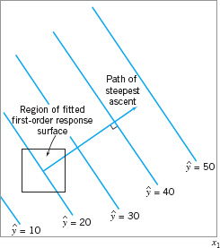
![]() FIGURE 14.3 First-order response surface and path of steepest ascent.
FIGURE 14.3 First-order response surface and path of steepest ascent.
EXAMPLE 14.1 An Application of Steepest Ascent
In Example 13.8, we described an experiment on a plasma etching process in which four factors were investigated to study their effect on the etch rate in a semiconductor water-etching application. We found that two of the four factors, the gap (x1) and the power (x4), significantly affected etch rate. Recall from that example that if we fit a model using only these main effects we obtain
ŷ = 776.0625 − 50.8125x1 + 153.0625x4
as a prediction equation for the etch rate.
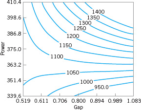
Figure 14.4 shows the contour plot from this model, over the original region of experimentation—that is, for gaps between 0.8 and 1.2 cm and power between 275 and 325 W. Note that within the original region of experimentation, the maximum etch rate that can be obtained is approximately 980 Å/m. The engineers would like to run this process at an etch rate of 1,100–1,150 Å/m. Use the method of steepest ascent to move away from the original region of experimentation to increase the etch rate.
SOLUTION
From examining the plot in Figure 14.4 (or the fitted model) we see that to move away from the design center—the point (x1 = 0, x2 = 0)—along the path of steepest ascent, we would move −50.8125 units in the x1 direction for every 153.0625 units in the x4 direction. Thus the path of steepest ascent passes through the point (x1 = 0, x2 = 0) and has slope 153.0625/ (−50.8125) ≅ −3. The engineer decides to use 25 W of power as the basic step size. Now, 25 W of power is equivalent to a step in the coded variable x4 of Δx4 = 1. Therefore, the steps along the path of steepest ascent are Δx4 = 1 and Δx1 = Δx4/(−3) = −0.33. A change of Δx1 = −0.33 in the coded variable x1 is equivalent to about −0.067 cm in the original variable gap.
Therefore, the engineer will move along the path of steepest ascent by increasing power by 25 W and decreasing gap by −0.067 cm. An actual observation on etch rate will be obtained by running the process at each point.
Figure 14.4 shows three points along this path of steepest ascent and the etch rates actually observed from the process at those points. At points A, B, and C, the observed etch rates increase steadily. At point C, the observed etch rate is 1,163 Å/m. Therefore, the steepest ascent procedure would terminate in the vicinity of power = 375 W and gap = 0.8 cm with an observed etch rate of 1,163 Å/m. This region is very close to the desired operating region for the process.

![]() FIGURE 14.4 Steepest ascent experiment for Example 14.1.
FIGURE 14.4 Steepest ascent experiment for Example 14.1.
14.1.2 Analysis of a Second-Order Response Surface
When the experimenter is relatively close to the optimum, a second-order model is usually required to approximate the response because of curvature in the true response surface. The fitted second-order response surface model is
![]()
where ![]() denotes the least squares estimate of β. In the next example, we illustrate how a fitted second-order model can be used to find the optimum operating conditions for a process, and how to describe the behavior of the response function.
denotes the least squares estimate of β. In the next example, we illustrate how a fitted second-order model can be used to find the optimum operating conditions for a process, and how to describe the behavior of the response function.
EXAMPLE 14.2 Continuation of Example 14.1
Recall that in applying the method of steepest ascent to the plasma etching process in Example 14.1 we had found a region near gap = 0.8 cm and power = 375 W, which would apparently give etch rates near the desired target of between 1100 and 1150 Å/m. The experimenters decided to explore this region more closely by running an experiment that would support a second-order response surface model. Table 14.1 and Figure 14.5 show the experimental design, centered at gap = 0.8 cm and power = 375 W, which consists of a 22 factorial design with four center points and four runs located along the coordinate axes called axial runs. The resulting design is called a central composite design, and it is widely used in practice for fitting second-order response surfaces.
Two response variables were measured during this phase of the study: etch rate (in Å/m) and etch uniformity (this is the standard deviation of the thickness of the layer of material applied to the surface of the wafer after it has been etched to a particular average thickness). Determine optimal operating conditions for this process.
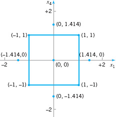
![]() FIGURE 14.5 Central composite design in the coded variables for Example 14.2.
FIGURE 14.5 Central composite design in the coded variables for Example 14.2.
![]() TABLE 14.1
TABLE 14.1
Central Composite Design of Example 14.2

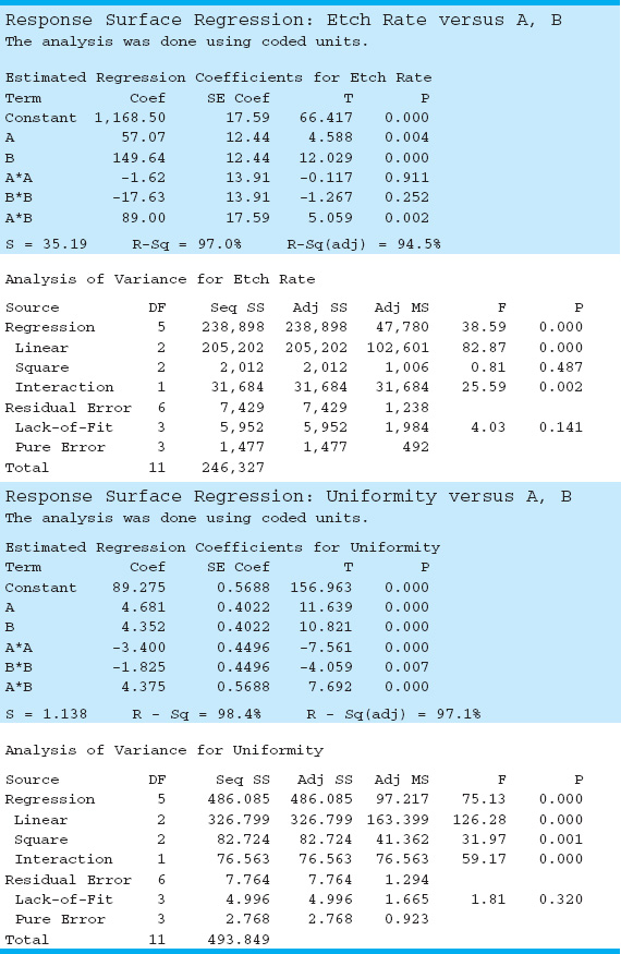
Minitab can be used to analyze the data from this experiment. The Minitab output is in Table 14.2.
The second-order model fit to the etch rate response is
![]()
However, we note from the t-test statistics in Table 14.2 that the quadratic terms ![]() and
and ![]() are not statistically significant. Therefore, the experimenters decided to model etch rate with a first-order model with interaction:
are not statistically significant. Therefore, the experimenters decided to model etch rate with a first-order model with interaction:
ŷ1 = 1,155.7 + 57.1x1 + 149.7x4 + 89x1x4
Figure 14.6 shows the contours of constant etch rate from this model. There are obviously many combinations of x1 (gap) and x4 (power) that will give an etch rate in the desired range of 1,100–1,150 Å/m.
The second-order model for uniformity is
![]()
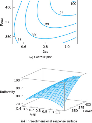
Table 14.2 gives the t-statistics for each model term. Since all terms are significant, the experimenters decided to use the quadratic model for uniformity. Figure 14.7 gives the contour plot and response surface for uniformity.
As in most response surface problems, the experimenter in this example had conflicting objectives regarding the two responses. One objective was to keep the etch rate within the acceptable range of 1,100 ≤ y1 ≤ 1,150 but to simultaneously minimize the uniformity. Specifically, the uniformity must not exceed y2 = 80, or many of the wafers will be defective in subsequent processing operations. When there are only a few independent variables, an easy way to solve this problem is to overlay the response surfaces to find the optimum. Figure 14.8 presents the overlay plot of both responses, with the contours of ŷ1 = 100, ŷ1 = 150, and ŷ2 = 80 shown. The shaded areas on this plot identify infeasible combinations of gap and power. The graph indicates that several combinations of gap and power should result in acceptable process performance.
![]() FIGURE 14.6 Contours of constant predicted etch rate, Example 14.2.
FIGURE 14.6 Contours of constant predicted etch rate, Example 14.2.
![]() FIGURE 14.7 Plots of the uniformity response, Example 14.2.
FIGURE 14.7 Plots of the uniformity response, Example 14.2.

![]() FIGURE 14.8 Overlay of the etch rate and uniformity response surfaces in Example 14.2 showing the region of the optimum (unshaded region).
FIGURE 14.8 Overlay of the etch rate and uniformity response surfaces in Example 14.2 showing the region of the optimum (unshaded region).
![]() TABLE 14.2
TABLE 14.2
Minitab Analysis of the Central Composite Design in Example 14.2

![]() FIGURE 14.9 Central composite designs for k = 2 and k = 3.
FIGURE 14.9 Central composite designs for k = 2 and k = 3.
Example 14.2 illustrates the use of a central composite design (CCD) for fitting a second-order response surface model. These designs are widely used in practice because they are relatively efficient with respect to the number of runs required. In general, a CCD in k factors requires 2k factorial runs, 2k axial runs, and at least one center point (3 to 5 center points are typically used). Designs for k = 2 and k = 3 factors are shown in Figure 14.9.
The central composite design may be made rotatable design by proper choice of the axial spacing α in Figure 14.9. If the design is rotatable, the standard deviation of predicted response ŷ is constant at all points that are the same distance from the center of the design. For rotatability, choose α = (F)1/4, where F is the number of points in the factorial part of the design (usually F = 2k). For the case of k = 2 factors, α = (22)1/4 = 1.414, as was used in the design in Example 14.2. Figure 14.10 presents a contour plot and a surface plot of the standard deviation of prediction for the quadratic model used for the uniformity response. Note that the contours are concentric circles, implying that uniformity is predicted with equal precision for all points that are the same distance from the center of the design. Also, note that the precision of response estimation decreases with increasing distance from the design center.
The central composite design is the most widely used design for fitting a second-order response surface model. However, there are many other useful designs. Section S14.1 of the supplemental material for this chapter contains more details of designs for fitting response surfaces.
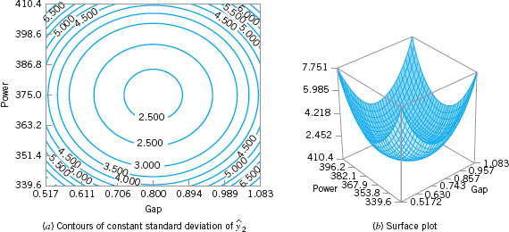
![]() FIGURE 14.10 Plots of constant standard deviation of predicted uniformity (y2), Example 14.2.
FIGURE 14.10 Plots of constant standard deviation of predicted uniformity (y2), Example 14.2.
14.2 Process Robustness Studies
14.2.1 Background
In Chapters 13 and 14, we have emphasized the importance of using statistically designed experiments for process design, development, and improvement. Over the past 30 years, engineers and scientists have become increasingly aware of the benefits of using designed experiments, and as a consequence there have been many new application areas. One of the most important of these is in process robustness studies, where the focus is on the following:
- Designing processes so that the manufactured product will be as close as possible to the desired target specifications even though some process variables (such as temperature), environmental factors (such as relative humidity), or raw material characteristics are impossible to control precisely.
- Determining the operating conditions for a process so that critical product characteristics are as close as possible to the desired target value and the variability around this target is minimized. Examples of this type of problem occur frequently. For instance, in semiconductor manufacturing we would like the oxide thickness on a wafer to be as close as possible to the target mean thickness, and we would also like the variability in thickness across the wafer (a measure of uniformity) to be as small as possible.
In the early 1980s, a Japanese engineer, Genichi Taguchi, introduced an approach to solving these types of problems, which he referred to as the robust parameter design (RPD) problem [see Taguchi and Wu (1980), Taguchi (1986)]. His approach was based on classifying the variables in a process as either control (or controllable) variables and noise (or uncontrollable) variables, and then finding the settings for the controllable variables that minimized the variability transmitted to the response from the uncontrollable variables. We make the assumption that although the noise factors are uncontrollable in the full-scale system, they can be controlled for purposes of an experiment. Refer to Figure 13.1 for a graphical view of controllable and uncontrollable variables in the general context of a designed experiment.
Taguchi introduced some novel statistical methods and some variations on established techniques as part of his RPD procedure. He made use of highly fractionated factorial designs and other types of fractional designs obtained from orthogonal arrays. His methodology generated considerable debate and controversy. Part of the controversy arose because Taguchi’s methodology was advocated in the West initially (and primarily) by consultants, and the underlying statistical science had not been adequately peer reviewed. By the late 1980s, the results of a very thorough and comprehensive peer review indicated that although Taguchi’s engineering concepts and the overall objective of RPD were well founded, there were substantial problems with his experimental strategy and methods of data analysis. For specific details of these issues, see Box, Bisgaard, and Fung (1988); Hunter (1985, 1987); Montgomery (1999); Myers, Montgomery, and Anderson-Cook (2009); and Pignatiello and Ramberg (1991). Many of these concerns are also summarized in the extensive panel discussion in the May 1992 issue of Technometrics [see Nair (1992)]. Section S14.2 of the supplemental material for this chapter also discusses and illustrates many of the problems underlying Taguchi’s technical methods.
Taguchi’s methodology for the RPD problem revolves around the use of an orthogonal design for the controllable factors that is “crossed” with a separate orthogonal design for the noise factors. Table 14.3 presents an example from Byrne and Taguchi (1987) that involved the development of a method to assemble an elastometric connector to a nylon tube that would deliver the required pull-off force. There are four controllable factors, each at three levels (A = interference, B = connector wall thickness, C = insertion depth, D = percent adhesive), and three noise or uncontrollable factors, each at two levels (E = conditioning time, F = conditioning temperature, G = conditioning relative humidity). Panel (a) of Table 14.3 contains the design for the controllable factors. Note that the design is a three-level fractional factorial; specifically, it is a 34−2 design. Taguchi calls this the inner array design. Panel (b) of Table 14.3 contains a 23 design for the noise factors, which Taguchi calls the outer array design. Each run in the inner array is performed for all treatment combinations in the outer array, producing the 72 observations on pull-off force shown in the table. This type of design is called a crossed array design.
![]() TABLE 14.3
TABLE 14.3
Taguchi Parameter Design with Both Inner and Outer Arrays [Byrne and Taguchi (1987)]
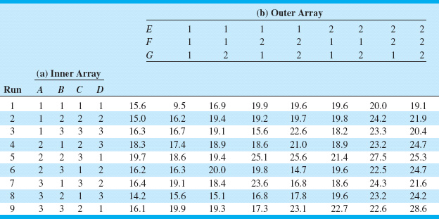
Taguchi suggested that we summarize the data from a crossed array experiment with two statistics: the average of each observation in the inner array across all runs in the outer array, and a summary statistic that attempted to combine information about the mean and variance, called the signal-to-noise ratio. These signal-to-noise ratios are purportedly defined so that a maximum value of the ratio minimizes variability transmitted from the noise variables. Then an analysis is performed to determine which settings of the controllable factors result in (1) the mean as close as possible to the desired target and (2) a maximum value of the signal-to-noise ratio.
Examination of Table 14.3 reveals a major problem with the Taguchi design strategy; namely, the crossed array approach will lead to a very large experiment. In our example, there are only seven factors, yet the design has 72 runs. Furthermore, the inner array design is a 34−2 resolution III design [see Montgomery (2009), Chapter 9, for discussion of this design], so in spite of the large number of runs, we cannot obtain any information about interactions among the controllable variables. Indeed, even information about the main effects is potentially tainted, because the main effects are heavily aliased with the two-factor interactions. It also turns out that the Taguchi signal-to-noise ratios are problematic; maximizing the ratio does not necessarily minimize variability. Refer to the supplemental text material for more details.
An important point about the crossed array design is that it does provide information about controllable factor × noise factor interactions. These interactions are crucial to the solution of an RPD problem. For example, consider the two-factor interaction graphs in Figure 14.11, where x is the controllable factor and z is the noise factor. In Figure 14.11a, there is no x × z interaction; therefore, there is no setting for the controllable variable x that will affect the variability transmitted to the response by the variability in z. However, in Figure 14.11b there is a strong x × z interaction. Note that when x is set to its low level there is much less variability in the response variable than when x is at the high level. Thus, unless there is at least one controllable factor × noise factor interaction, there is no robust design problem. As we will see in the next section, focusing on identifying and modeling these interactions is one of the keys to a more efficient and effective approach to investigating process robustness.

![]() FIGURE 14.11 The role of the control × noise interaction in robust design.
FIGURE 14.11 The role of the control × noise interaction in robust design.
14.2.2 The Response Surface Approach to Process Robustness Studies
As noted in the previous section, interactions between controllable and noise factors are the key to a process robustness study. Therefore, it is logical to utilize a model for the response that includes both controllable and noise factors and their interactions. To illustrate, suppose that we have two controllable factors x1 and x2 and a single noise factor z1. We assume that both control and noise factors are expressed as the usual coded variables; that is, they are centered at zero and have lower and upper limits at ±1. If we wish to consider a first-order model involving the controllable variables, then a logical model is
Note that this model has the main effects of both controllable factors, the main effect of the noise variable, and both interactions between the controllable and noise variables. This type of model incorporating both controllable and noise variables is often called a response model. Unless at least one of the regression coefficients δ11 and δ21 is nonzero, there will be no robust design problem.
An important advantage of the response model approach is that both the controllable factors and the noise factors can be placed in a single experimental design; that is, the inner and outer array structure of the Taguchi approach can be avoided. We usually call the design containing both controllable and noise factors a combined array design.
As mentioned previously, we assume that noise variables are random variables, although they are controllable for purposes of an experiment. Specifically, we assume that the noise variables are expressed in coded units, that they have expected value zero, variance σ2z, and that if there are several noise variables, they have zero covariances. Under these assumptions, it is easy to find a model for the mean response just by taking the expected value of y in equation 14.4. This yields
Ez(y) = β0 + β1x1 + β2x2 + β12x1x2
where the z subscript on the expectation operator is a reminder to take the expected value with respect to both random variables in equation 14.4, z1 and ε. To find a model for the variance of the response y, first rewrite equation 14.4 as follows:
y = β0 + β1x1 + β2x2 + β12x1x2 + (γ1 + δ11x1 + δ22x2)z1 + ε
Now the variance of y can be obtained by applying the variance operator across this last expression. The resulting variance model is
![]()
Once again, we have used the z subscript on the variance operator as a reminder that both z1 and ε are random variables.
We have derived simple models for the mean and variance of the response variable of interest. Note the following:
- The mean and variance models involve only the controllable variables. This means that we can potentially set the controllable variables to achieve a target value of the mean and minimize the variability transmitted by the noise variable.
- Although the variance model involves only the controllable variables, it also involves the interaction regression coefficients between the controllable and noise variables. This is how the noise variable influences the response.
- The variance model is a quadratic function of the controllable variables.
- The variance model (apart from σ2) is simply the square of the slope of the fitted response model in the direction of the noise variable.
To use these models operationally, we would:
- Perform an experiment and fit an appropriate response model such as equation 14.4.
- Replace the unknown regression coefficients in the mean and variance models with their least squares estimates from the response model and replace σ2 in the variance model by the residual mean square found when fitting the response model.
- Simultaneously optimize the mean and variance models. Often this can be done graphically. For more discussion of other optimization methods, refer to Myers, Montgomery, and Anderson-Cook (2009).
It is very easy to generalize these results. Suppose that there are k controllable variables x′ = [x1, x2, …, xk ], and r noise variables z′ = [z1, z2, …, zr]. We will write the general response model involving these variables as
where f(x) is the portion of the model that involves only the controllable variables and h(x, z) are the terms involving the main effects of the noise factors and the interactions between the controllable and noise factors. Typically, the structure for h(x, z) is
![]()
The structure for f(x) will depend on what type of model for the controllable variables the experimenter thinks is appropriate. The logical choices are the first-order model with interaction and the second-order model. If we assume that the noise variables have mean zero, variance ![]() , and zero covariances, and that the noise variables and the random errors ε have zero covariances, then the mean model for the response is simply
, and zero covariances, and that the noise variables and the random errors ε have zero covariances, then the mean model for the response is simply
To find the variance model, we will use the transmission of error approach from Section 8.7.2. This involves first expanding equation 14.5 around z = 0 in a first-order Taylor series:
![]()
where R is the remainder. If we ignore the remainder and apply the variance operator to this last expression, the variance model for the response is
Myers, Montgomery, and Anderson-Cook (2009) give a slightly more general form for equation 14.7 based on applying a conditional variance operator directly to the response model in equation 14.5.
To illustrate a process robustness study, consider an experiment [described in detail in Montgomery (2009)] in which four factors were studied in a 24 factorial design to investigate their effect on the filtration rate of a chemical product. We will assume that factor A, temperature, is hard to control in the full-scale process but it can be controlled during the experiment (which was performed in a pilot plant). The other three factors— pressure (B), concentration (C), and stirring rate (D)—are easy to control. Thus the noise factor z1 is temperature and the controllable variables x1, x2, and x3 are pressure, concentration, and stirring rate, respectively. The experimenters conducted the (unreplicated) 24 design shown in Table 14.4. Since both the controllable factors and the noise factor are in the same design, the 24 factorial design used in this experiment is an example of a combined array design. We want to determine operating conditions that maximize the filtration rate and minimize the variability transmitted from the noise variable temperature.
![]() TABLE 14.4
TABLE 14.4
Pilot Plant Filtration Rate Experiment

Using the methods for analyzing a 2k factorial design from Chapter 13, the response model is
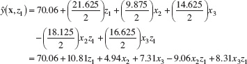
Using equations 14.6 and 14.7, we can find the mean and variance models as
Ez[y(x, z1)] = 70.06 + 4.94x2 + 7.31x3
and

respectively. Now assume that the low and high levels of the noise variable temperature have been run at one standard deviation either side of its typical or average value, so that ![]() , and use
, and use ![]() (this is the residual mean square obtained by fitting the response model). Therefore, the variance model becomes
(this is the residual mean square obtained by fitting the response model). Therefore, the variance model becomes
![]()
Figure 14.12 presents a contour plot of the response contours from the mean model. To construct this plot, we held the noise factor (temperature) at zero and the nonsignificant controllable factor (pressure) at zero. Note that mean filtration rate increases as both concentration and stirring rate increase. The square root of Vz[y(x, z)] is plotted in Figure 14.13. Note that both a contour plot and a three-dimensional response surface plot are given. This plot was also constructed by setting the noise factor temperature and the nonsignificant controllable factor to zero.

![]() FIGURE 14.12 Contours of constant mean filtration rate, Example 14.3, with z1 = temperature = 0.
FIGURE 14.12 Contours of constant mean filtration rate, Example 14.3, with z1 = temperature = 0.
Suppose that the experimenter wants to maintain mean filtration rate above 75 and minimize the variability around this value. Figure 14.14 shows an overlay plot of the contours of mean filtration rate and the square root of Vz[y(x, z)] as a function of concentration and stirring rate, the significant controllable variables. To achieve the desired objectives, it will be necessary to hold concentration at the high level and stirring rate very near the middle level.

![]() FIGURE 14.13 Contour plot and response surface of
FIGURE 14.13 Contour plot and response surface of ![]() for Example 14.3, with z1 = temperature = 0.
for Example 14.3, with z1 = temperature = 0.
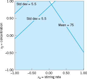
![]() FIGURE 14.14 Overlay plot of mean and standard deviation for filtration rate, Example 14.4, with z1 = temperature = 0.
FIGURE 14.14 Overlay plot of mean and standard deviation for filtration rate, Example 14.4, with z1 = temperature = 0.
Example 14.3 illustrates the use of a first-order model with interaction as the model for the controllable factors, f (x). In Example 14.4, we present a second-order model.
EXAMPLE 14.4 Robust Manufacturing
A process robustness study was conducted in a semiconductor manufacturing plant involving two controllable variables x1 and x2 and a single noise factor z. Table 14.5 shows the experiment that was performed, and Figure 14.15 gives a graphical view of the design. Note that the experimental design is a “modified” central composite design in which the axial runs in the z direction have been eliminated. It is possible to delete these runs because no quadratic term (z2) in the noise variable is included in the model. The objective is to find operating conditions that give a mean response between 90 and 100, while making the variability transmitted from the noise variable as small as possible.
![]() TABLE 14.5
TABLE 14.5
The Modified Central Composite Design for the Process Robustness Study in Example 14.4

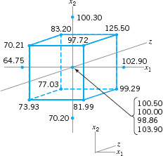
![]() FIGURE 14.15 The Modified central composite design in Example 14.4.
FIGURE 14.15 The Modified central composite design in Example 14.4.
Using equation 14.5, the response model for this process robustness study is
The least squares fit is
![]()
Therefore, from equation 14.6, the mean model is
![]()
![]() FIGURE 14.16 Plots of the mean model, Example 14.4.
FIGURE 14.16 Plots of the mean model, Example 14.4.
Using equation 14.7, the variance model is

We will assume (as in the previous example) that ![]() and since the residual mean square from fitting the response model is MSE = 3.73, we will use
and since the residual mean square from fitting the response model is MSE = 3.73, we will use ![]() . Therefore, the variance model is
. Therefore, the variance model is
Vz[y(x, z)] = (5.55 + 4.94x1 + 2.55x2)2 + 3.73
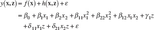
Figures 14.16 and 14.17 show response surface contour plots and three-dimensional surface plots of the mean model and the standard deviation ![]() , respectively.
, respectively.

![]() FIGURE 14.17 Plots of the standard deviation of the response
FIGURE 14.17 Plots of the standard deviation of the response ![]() , Example 14.4.
, Example 14.4.
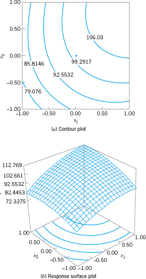
The objective of the experimenters in this process robustness study was to find a set of operating conditions that would result in a mean response between 90 and 100 with low variability. Figure 14.18 is an overlay of the contours 90 and 100 from the mean model with the contour of constant standard deviation of 4. The unshaded region of this plot indicates operating conditions on x1 and x2, where the requirements for the mean response are satisfied and the response standard deviation does not exceed 4.
![]() FIGURE 14.18 Overlay of the mean and standard deviation contours, Example 14.4.
FIGURE 14.18 Overlay of the mean and standard deviation contours, Example 14.4.
14.3 Evolutionary Operation
Most process-monitoring techniques measure one or more output quality characteristics, and if these quality characteristics are satisfactory, no modification of the process is made. However, in some situations where there is a strong relationship between one or more controllable process variables and the observed quality characteristic or response variable, other process-monitoring methods can sometimes be employed. For example, suppose that a chemical engineer wishes to maximize the yield of the process. The yield is a function of two controllable process variables, temperature (x1) and time (x2)—say,
y = f (x1, x2) + ε
where ε is a random error component. The chemical engineer has found a set of operating conditions or levels for x1 and x2 that maximizes yield and provides acceptable values for all other quality characteristics. This process optimization may have been done using RSM; however, even if the plant operates continuously at these levels, it will eventually “drift” away from the optimum as a result of variations in the incoming raw materials, environmental changes, operating personnel, and the like.
A method is needed for continuous operation and monitoring of a process with the goal of moving the operating conditions toward the optimum or following a “drift.” The method should not require large or sudden changes in operating conditions that might disrupt production. Evolutionary operation (EVOP) was proposed by Box (1957) as such an operating procedure. It is designed as a method of routine plant operation that is carried out by operating personnel with minimum assistance from the quality or manufacturing engineering staff. EVOP makes use of principles of experimental design, which usually is considered to be an off-line quality-engineering method. Thus, EVOP is an on-line application of designed experiments.
![]() FIGURE 14.19 22 factorial design.
FIGURE 14.19 22 factorial design.
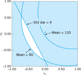
EVOP consists of systematically introducing small changes in the levels of the process operating variables. The procedure requires that each independent process variable be assigned a “high” and a “low” level. The changes in the variables are assumed to be small enough so that serious disturbances in product quality will not occur, yet large enough so that potential improvements in process performance will eventually be discovered. For two variables x1 and x2, the four possible combinations of high and low levels are shown in Figure 14.19. This arrangement of points is the 22 factorial design introduced in Chapter 13. We have also included a point at the center of the design. Typically, the 22 design would be centered about the best current estimate of the optimum operating conditions.
The points in the 22 design are numbered 1, 2, 3, 4, and 5. Let y1, y2, y3, y4, and y5 be the observed values of the dependent or response variable corresponding to these points. After one observation has been run at each point in the design, an EVOP cycle is said to have been completed. Recall that the main effect of a factor is defined as the average change in response produced by a change from the low level to the high level of the factor. Thus, the effect of x1 is the average difference between the responses on the right-hand side of the design in Figure 14.19 and the responses on the left-hand side, or

Similarly, the effect of x2 is found by computing the average difference in the responses on the top of the design in Figure 14.19 and the responses on the bottom—that is,
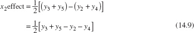
If the change from the low to the high level of x1 produces an effect that is different at the two levels of x2, then there is interaction between x1 and x2. The interaction effect is
or simply the average difference between the diagonal totals in Figure 14.19. After n cycles, there will be n observations at each of the five design points. The effects of x1, x2, and their interaction are then computed by replacing the individual observations yi, in equations 14.8, 14.9, and 14.10 by the averages ![]() of the n observations at each point.
of the n observations at each point.
After several cycles have been completed, one or more process variables, or their interaction, may appear to have a significant effect on the response variable y. When this occurs, a decision may be made to change the basic operating conditions to improve the process output. When improved conditions are detected, an EVOP phase is said to have been completed.
In testing the significance of process variables and interactions, an estimate of experimental error is required. This is calculated from the cycle data. By comparing the response at the center point with the 2k points in the factorial portion, we may check on the presence of curvature in the response function; that is, if the process is really centered at the maximum (say), then the response at the center should be significantly greater than the responses at the 2k peripheral points.
In theory, EVOP can be applied to an arbitrary number of process variables. In practice, only two or three variables are usually considered at a time. Example 14.5 shows the procedure for two variables. Box and Draper (1969) give a discussion of the three-variable case, including necessary forms and worksheets. EVOP calculations can be easily performed in statistical software packages for factorial designs.
EXAMPLE 14.5 Two-Variable EVOP
Consider a chemical process whose yield is a function of temperature (x1) and pressure (x2). The current operating conditions are x1 = 250°F and x2 = 145 psi. The EVOP procedure uses the 22 design plus the center point shown in Figure 14.20. The cycle is completed by running each design point in numerical order (1, 2, 3, 4, 5). The yields in the first cycle are shown in Figure 14.20. Set up the EVOP procedure.
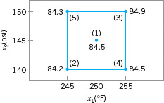
![]() FIGURE 14.20 22 design for Example 14.5.
FIGURE 14.20 22 design for Example 14.5.
SOLUTION
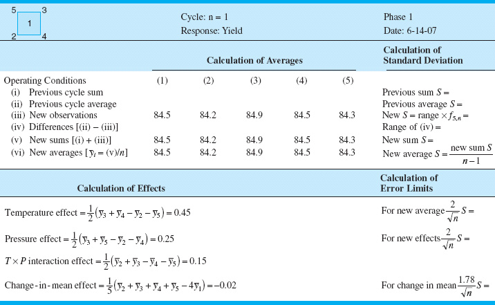
The yields from the first cycle are entered in the EVOP calculation sheet shown in Table 14.6. At the end of the first cycle, no estimate of the standard deviation can be made. The calculation of the main effects of temperature and pressure and their interaction are shown in the bottom half of Table 14.6.
A second cycle is then run, and the yield data are entered in another EVOP calculation sheet shown in Table 14.7. At the end of the second cycle, the experimental error can be estimated and the estimates of the effects compared to approximate 95% (two standard deviation) limits. Note that the range refers to the range of the differences in row (iv); thus, the range is +1.0 −(−1.0) = 2.0. Since none of the effects in Table 14.7 exceeds their error limits, the true effect is probably zero, and no changes in operating conditions are contemplated.
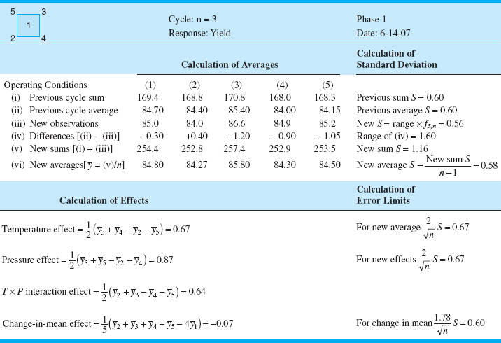
The results of a third cycle are shown in Table 14.8. The effect of pressure now exceeds its error limit, and the temperature effect is equal to the error limit. A change in operating conditions is now probably justified.
In light of the results, it seems reasonable to begin a new EVOP phase about point (3). Thus, x1 = 225°F and x2 = 150 psi would become the center of the 22 design in the second phase.
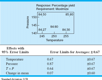
An important aspect of EVOP is feeding the information generated back to the process operators and supervisors. This is accomplished by a prominently displayed EVOP information board. The information board for this example at the end of cycle three is shown in Table 14.9.
![]() TABLE 14.6
TABLE 14.6
EVOP Calculation Sheet—Example 14.5, n = 1
![]() TABLE 14.7
TABLE 14.7
EVOP Calculation Sheet—Example 14.5, n = 2

![]() TABLE 14.8
TABLE 14.8
EVOP Calculation Sheet—Example 14.5, n = 3
![]() TABLE 14.9
TABLE 14.9
EVOP Information Board—Cycle Three
Most of the quantities on the EVOP calculation sheet follow directly from the analysis of the 2k factorial design. For example, the variance of any effect such as ![]() is simply
is simply
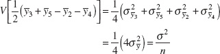
where σ2 is the variance of the observations (y). Thus, two standard deviation (corresponding to approximately 95%) error limits on any effect would be ![]() . The variance of the change in mean is
. The variance of the change in mean is

Thus, two standard deviation error limits on the CIM are ![]() . For more information on the 2k factorial design, see Chapter 13 and Montgomery (2009).
. For more information on the 2k factorial design, see Chapter 13 and Montgomery (2009).
The standard deviation σ is estimated by the range method. Let yi(n) denote the observation at the ith design point in cycle n, and ![]() the corresponding average of yi(n) after n cycles. The quantities in row (iv) of the EVOP calculation sheet are the differences
the corresponding average of yi(n) after n cycles. The quantities in row (iv) of the EVOP calculation sheet are the differences ![]() . The variance of these differences is
. The variance of these differences is ![]() . The range of the differences—say, RD—is related to the estimate of the distribution of the differences by
. The range of the differences—say, RD—is related to the estimate of the distribution of the differences by ![]() . Now
. Now ![]() , so
, so
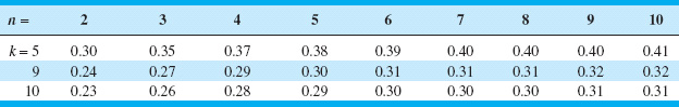
![]()
can be used to estimate the standard deviation of the observations, where k denotes the number of points used in the design. For a 22 with one center point we have k = 5, and for a 23 with one center point we have k = 9. Values of fk, n are given in Table 14.10.
Important Terms and Concepts
Central composite design
Combined array design
Contour plot
Controllable variable
Crossed array design
Evolutionary operation (EVOP)
EVOP cycle
EVOP phase
First-order model
Inner array design
Method of steepest ascent
Noise variable
Outer array design
Path of steepest ascent
Response model
Response surface
Response surface methodology (RSM)
Robust parameter design (RPD)
Rotatable design
Second-order model
Sequential experimentation
Taylor series
Transmission of error
Exercises
![]()
The Student Resource Manual presents comprehensive annotated solutions to the odd-numbered exercises included in the Answers to Selected Exercises section in the back of this book
14.1. Discuss why a central composite design would almost always be preferable to a 3k factorial design for fitting a second-order response surface model.
14.2. Sometimes experimenters prefer to use a spherical central composite design in which the axial distance is ![]() , where k is the number of design factors. Is the spherical design similar to the rotatable design? Are there cases where the spherical design is also rotatable?
, where k is the number of design factors. Is the spherical design similar to the rotatable design? Are there cases where the spherical design is also rotatable?
14.3. Consider the first-order model
ŷ = 75 + 10x1 + 6x2
(a) Sketch the contours of constant predicted response over the range −1 ≤ xi ≤ +1, i = 1, 2.
(b) Find the direction of steepest ascent.
14.4. Consider the first-order model
ŷ = 50 + 2x1 − 15x2 + 3x3
where −1 ≤xi ≤+1, i = 1, 2, 3. Find the direction of steepest ascent.
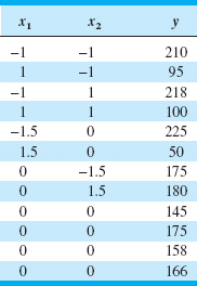
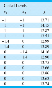
14.5. An experiment was run to study the effect of two factors—time and temperature—on the inorganic impurity levels in paper pulp. The results of this experiment are shown in Table 14E.1.
(a) What type of experimental design has been used in this study? Is the design rotatable?
(b) Fit a quadratic model to the response, using the method of least squares.
(c) Construct the fitted impurity response surface. What values of x1 and x2 would you recommend if you wanted to minimize the impurity level?
(d) Suppose that
![]()
where temperature is in °C and time is in hours. Find the optimum operating conditions in terms of the natural variables temperature and time.
![]() TABLE 14E.1
TABLE 14E.1
The Experiment for Exercise 14.5
14.6. A second-order response surface model in two variables is
![]()
(a) Generate a two-dimensional contour plot for this model over the region −2 ≤xi ≤ +2, i = 1, 2, and select the values of x1 and x2 that maximize ŷ .
(b) Find the two equations given by
![]()
Show that the solution to these equations for the optimum conditions x1 and x2 are the same as those found graphically in part (a).
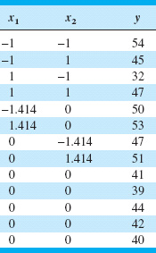
14.7. An article in Rubber Chemistry and Technology (Vol. 47, 1974, pp. 825–836) describes an experiment that studies the relationship of the Mooney viscosity of rubber to several variables, including silica filler (parts per hundred) and oil filler (parts per hundred). Some of the data from this experiment are shown in Table 14E.2, where
![]()
(a) What type of experimental design has been used? Is it rotatable?
(b) Fit a quadratic model to these data. What values of x1 and x2 will maximize the Mooney viscosity?
![]() TABLE 14E.2
TABLE 14E.2
The Viscosity Experiment for Exercise 14.7
![]() TABLE 14E.3
TABLE 14E.3
The Experiment for Exercise 14.8

![]() TABLE 14E.4
TABLE 14E.4
The Spring Experiment for Exercise 14.9

14.8. In their book Empirical Model Building and Response Surfaces (John Wiley, New York; 1987), G. E. P. Box and N. R. Draper describe an experiment with three factors. The data shown in Table 14E.3 are a variation of the original experiment on p. 247 of their book. Suppose that these data were collected in a semiconductor manufacturing process.
(a) The response y1 is the average of three readings on resistivity for a single wafer. Fit a quadratic model to this response.
(b) The response y2 is the standard deviation of the three resistivity measurements. Fit a first-order model to this response.
(c) Where would you recommend that we set x1, x2, and x3 if the objective is to hold mean resistivity at 500 and minimize the standard deviation?
14.9. An article by J. J. Pignatiello, Jr., and J. S. Ramberg in the Journal of Quality Technology (Vol. 17, 1985, pp. 198–206) describes the use of a replicated fractional factorial to investigate the effect of five factors on the free height of leaf springs used in an automotive application. The factors are A = furnace temperature, B = heating time, C = transfer time, D = hold down time, and E = quench oil temperature. The data are shown in Table 14E.4.
(a) Write out the alias structure for this design. What is the resolution of this design?
(b) Analyze the data. What factors influence mean free height?
(c) Calculate the range and standard deviation of free height for each run. Is there any indication that any of these factors affects variability in free height?
(d) Analyze the residuals from this experiment and comment on your findings.
(e) Is this the best possible design for five factors in 16 runs? Specifically, can you find a fractional design for five factors in 16 runs with higher resolution than this one?
14.10. Consider the leaf spring experiment in Exercise 14.9. Suppose that factor E (quench oil temperature) is very difficult to control during manufacturing. We want to have the mean spring height as close to 7.50 as possible with minimum variability. Where would you set factors A, B, C, and D to reduce variability in free height as much as possible regardless of the quench oil temperature used?
14.11. Consider the leaf spring experiment in Exercise 14.9. Rework this problem, assuming that factors A, B, and C are easy to control but factors D and E are hard to control.
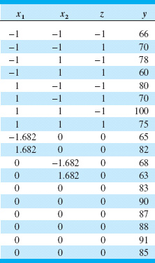
14.12. The data shown in the Table 14E.5 were collected in an experiment to optimize crystal growth as a function of three variables x1, x2, and x3. Large values of y (yield in grams) are desirable. Fit a second-order model and analyze the fitted surface. Under what set of conditions is maximum growth achieved?
![]() TABLE 14E.5
TABLE 14E.5
Crystal Growth Experiment for Exercise 14.12

![]() TABLE 14E.6
TABLE 14E.6
Chemical Process Experiment for Exercise 14.13
14.13. The data in Table 14E.6 were collected by a chemical engineer. The response y is filtration time, x1 is temperature, and x2 is pressure. Fit a second-order model.
(a) What operating conditions would you recommend if the objective is to minimize the filtration time?
(b) What operating conditions would you recommend if the objective is to operate the process at a mean filtration rate very close to 46?
14.14. Reconsider the crystal growth experiment from Exercise 14.12. Suppose that x3 = z is now a noise variable, and that the modified experimental design shown in Table 14E.7 has been conducted. The experimenters want the growth rate to be as large as possible, but they also want the variability transmitted from z to be small. Under what set of conditions is growth greater than 90 with minimum variability achieved?
14.15. An article in Quality Progress (“For Starbucks, It’s in the Bag,” March 2011, pp. 18–23) describes using a central composite design to improve the packaging of one-pound coffee. The objective is to produce an airtight seal that is easy to open without damaging the top of the coffee bag. The experimenters studied three factors—x1 = plastic viscosity (300–400 centipoise), x2 = clamp pressure (170–190 psi), and x3 = plate gap (−3, +3 mm)—and two responses, y1 = tear and y2 = leakage. The design is shown in Table 14E.8.
![]() TABLE 14E.7
TABLE 14E.7
Crystal Growth Experiment for Exercise 14.14
![]() TABLE 14E.8
TABLE 14E.8
The Coffee Bag Experiment in Exercise 14.15
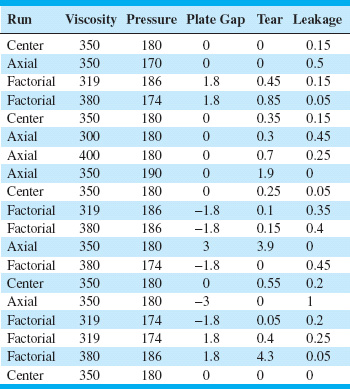
The tear response was measured on a scale from 0–9 (good to bad), and leakage was proportion failing. Each run used a sample of 20 bags for response measurement.
(a) Build a second-order model for the tear response.
(b) Build a second-order model for the leakage response.
(c) Analyze the residuals for both models. Do transformations seem necessary for either response? If so, refit the models in the transformed metric.
(d) Construct response surface plots and contour plots for both responses. Provide interpretations for the fitted surfaces.
(e) What conditions would you recommend for process operation to minimize leakage and keep tear below 0.75?
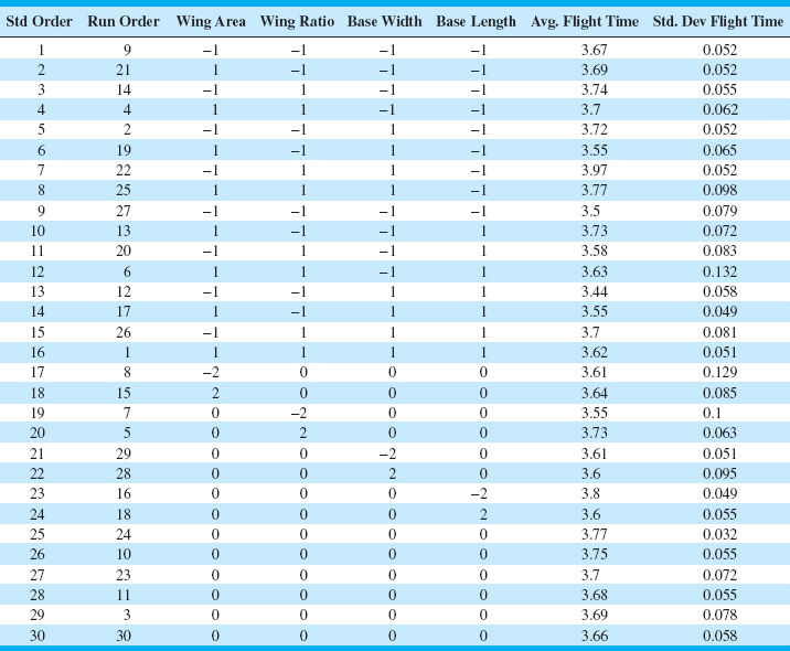
14.16. Box and Liu (1999) describe an experiment flying paper helicopters where the objective is to maximize flight time. They used the central composite design shown in Table 14E.9. Each run involved a single helicopter made to the following specifications: x1 = wing area (in2),−1 = 11.80 and +1 = 13.00; x2 = wing-length-to-width ratio, −1 = 2.25 and +1 = 2.78; x3 = base width (in), −1 = 1.00 and +1 = 1.50; and x4 = base length (in), −1 = 1.50 and +1 = 2.50. Each helicopter was flown four times, and the average flight time and the standard deviation of flight time were recorded.
(a) Fit a second-order model to the average flight-time response.
(b) Fit a second-order model to the standard deviation of flight-time response.
(c) Analyze the residuals for both models from parts (a) and (b). Are transformations on the response(s) necessary? If so, fit the appropriate models.
(d) What design would you recommend to maximize the flight time?
(e) What design would you recommend to maximize the flight time while simultaneously minimizing the standard deviation of flight time?
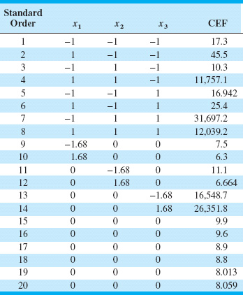
14.17. An article in the Journal of Chromatography A (“Optimization of the Capillary Electrophoresis Separation of Ranitidine and Related Compounds,” Vol. 766, pp. 245–254) describes an experiment to optimize the production of ranitidine, a compound that is the primary active ingredient of Zantac, a pharmaceutical product used to treat ulcers, gastroesophageal reflux disease (a condition in which backward flow of acid from the stomach causes heartburn and injury of the esophagus), and other conditions where the stomach produces too much acid, such as Zollinger-Ellison syndrome. The authors used three factors (x1 = pH of the buffer solution, x2 = the electrophoresis voltage, and the concentration of one component of the buffer solution) in a central composite design. The response is chromatographic exponential function (CEF), which should be minimized. Table 14E.10 shows the design.
(a) Fit a second-order model to the CEF response. Analyze the residuals from this model. Does it seem that all model terms are necessary?
(b) Reduce the model from part (a) as necessary. Did model reduction improve the fit?
(c) Does transformation of the CEF response seem like a useful idea? What aspect of either the data or the residual analysis suggests that transformation would be helpful?
(d) Fit a second-order model to the transformed CEF response. Analyze the residuals from this model. Does it seem that all model terms are necessary? What would you choose as the final model?
(e) What conditions would you recommend using to minimize CEF?
![]() TABLE 14E.9
TABLE 14E.9
The Paper Helicopter Experiment
14.18. An article in the Electronic Journal of Biotechnology (“Optimization of Medium Composition for Transglutaminase Production by a Brazilian Soil Streptomyces sp.,”) describes the use of designed experiments to improve the medium for cells used in a new microbial source of transglutaminase (MTGase), an enzyme that catalyzes an acyl transfer reaction using peptide-bond glutamine residues as acyl donors and some primary amines as acceptors. Reactions catalyzed by MTGase can be used in food processing. The article describes two phases of experimentation: screening with a fractional factorial, and optimization. We will use only the optimization experiment. The design was a central composite design in four factors: x1 = KH2PO4, x2 = MgSO47H2O, x3 = soybean flower, and x4 = peptone. MTGase activity is the response, which should be maximized. Table 14E.11 contains the design and the response data.
(a) Fit a second-order model to the MTGase activity response.
(b) Analyze the residuals from this model.
(c) Recommend operating conditions that maximize MTGase activity.
14.19. Consider the response model in equation 14.5 and the transmission of error approach to finding the variance model (equation 14.7). Suppose that in the response model we use
![]()
![]() TABLE 14E.10
TABLE 14E.10
The Ranitidine Separation Experiment
![]() TABLE 14E.11
TABLE 14E.11
The MTGase Optimization Experiment for Exercise 14.18

What effect does including the interaction terms between the noise variables have on the variance model?
14.20. Consider the response model in equation 14.5. Suppose that in the response model we allow for a complete second-order model in the noise factors so that

What effect does this have on the variance model?