
Answers to
Selected Exercises
3.1. (a) ![]() = 16.029. (b) s = 0.0202.
= 16.029. (b) s = 0.0202.
3.5. (a) ![]() = 952.9. (b) s = 3.7.
= 952.9. (b) s = 3.7.
3.7. (a) ![]() = 121.25. (b) s = 22.63.
= 121.25. (b) s = 22.63.
3.15. Both the normal and lognormal distributions appear to be reasonable models for the data.
3.17. The lognormal distribution appears to be a reasonable model for the concentration data.
3.23. (a) ![]() = 89.476. (b) s = 4.158.
= 89.476. (b) s = 4.158.
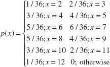
3.27. sample space: {2, 3, 4, 5, 6, 7, 8, 9, 10, 11, 12}
(c) Cutting occurrence rate reduces probability from 0.0198 to 0.0100.
3.31. (a) k = 0.05. (b) µ = 1.867, σ2 = 0.615.
(c) F(x) = {0.383; x = 1 0.750; x = 2 1.000; x = 3
3.33. (a) Approximately 11.8%. (b) Decrease profit by $5.90/calculator.
3.35. Decision rule means 22% of samples will have one or more nonconforming units.
3.43. (a) 0.633. (b) 0.659. Approximation is not satisfactory.
(c) n/N = 0.033. Approximation is satisfactory.
(d) n = 11
3.45. Pr{x = 0} = 0.364, Pr{x ≥ 2 } = 0.264
3.51. Pr{x ≤ 35} = 0.159. Number failing minimum spec is 7950.
Pr{x > 48} = 0.055. Number failing maximum spec is 2750.
3.53. Process is centered at target, so shifting process mean in either direction increases nonconformities. Process variance must be reduced to 0.0152 to have at least 999 of 1000 conform to specification.
3.57. If c2 > c1 + 0.0620, then choose process 1.
(b) P = 0.0629
(c) P = 0.0404
(d) P = 0.0629
(b) P = 0.0233
(c) P = 0.0146
(d) P = 0.0322
(b) 0.025 < P < 0.25
(c) 0.025 < P < 0.05
(d) 0.005 < P < 0.001
4.7. (a) Z0 = 6.78. Reject H0.
(b) P = 0. (c) 8.249 ≤ µ ≤ 8.251.
4.9. (a) t0 = 1.952. Reject H0.
(b) 25.06 ≤ µ ≤ 26.94.
4.11. (a) t0 = –3.089. Reject H0.
(b) 13.39216 ≤ µ ≤ 13.40020.
4.15. (a) t0 = −6.971. Reject H0.
(b) 9.727 ≤ µ ≤ 10.792
(c) ![]() = 14.970. Do not reject H0.
= 14.970. Do not reject H0.
(d) 0.738 ≤ σ ≤1.546
(e) σ ≤ 1.436
4.17. (a) t0 = 0.11. Do not reject H0.
(c) −0.127 ≤ (µ1 − µ2) ≤ 0.141
(d) F0 = 0.8464. Do not reject H0.
(e) 0.165 ≤ ![]() ≤ 4.821
≤ 4.821
(f) 0.007 ≤ σ2 ≤ 0.065
4.19. (a) t0 = −0.77. Do not reject H0.
(b) −6.7 ≤ (µ1 − µ2) ≤ 3.1.
(c) 0.21 ≤ ![]() ≤ 3.34
≤ 3.34
4.21. (a) Z0 = 4.0387. Reject H0.
(b) P = 0.00006.
(c) p ≤ 0.155.
4.23. (a) F0 = 1.0987. Do not reject H0.
(b) t0 = 1.461. Do not reject H0.
4.25. t0 = −1.10. There is no difference between mean measurements.
4.27. (a) ![]() = 42.75. Do not reject H0.
= 42.75. Do not reject H0.
(b) 1.14 ≤ σ ≤ 2.19.
4.33. Z0 = 0.3162. Do not reject Ho.
4.35. (a) F0 = 3.59, P = 0.053.
4.37. (a) F0 = 1.87, P = 0.214.
4.39. (a) F0 = 1.45, P = 0.258.
4.41. (a) F0 = 30.85, P ≃ 0.000.
4.53. Z = 4.1667, P = 0.000031
(b) 0.01 < P < 0.025
(c) 0.01 < P < 0.005
(d) 0.025 < P < 0.05
(b) No
(c) (0.28212, 0.37121)
(d) P = 0.313/2 = 0.1565
4.61. Error DF = 12, MSFactor = 18.30,
MSError = 1.67, F = 10.96, 0.00094
5.19. There is a nonrandom, cyclic pattern.
5.21. Points 17, 18, 19, and 20 are outside lower 1-sigma area.
5.23. Points 16, 17, and 18 are 2 of 3 beyond 2 sigma of centerline. Points 5, 6, 7, 8, and 9 are of 5 at 1 sigma or beyond of centerline.
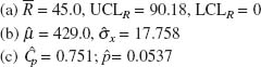
6.1. (a) ![]() chart: CL = 0.5138, UCL = 0.5507,
chart: CL = 0.5138, UCL = 0.5507,
LCL = 0.4769
R chart: CL = 0.0506, LCL = 0,
UCL = 0.0842
(b) ![]() = 0.5138,
= 0.5138, ![]() = 0.0246
= 0.0246
6.7. (a) Samples 12 and 15 exceed ![]() UCL.
UCL.
(b) ![]() = 0.00050.
= 0.00050.
6.9. (a) ![]() chart: CL = 10.9, UCL = 47.53,
chart: CL = 10.9, UCL = 47.53,
LCL = −25.73
R chart: CL = 63.5, UCL = 134.4, LCL = 0
Process is in statistical control.
(b) ![]() = 27.3. (c)
= 27.3. (c) ![]() = 1.22.
= 1.22.
6.11. (a) ![]() chart: CL = −0.003, UCL = 1.037,
chart: CL = −0.003, UCL = 1.037,
LCL = −1.043
s chart: CL = 1.066, UCL = 1.830,
LCL = 0.302
(b) R chart: CL = 3.2, UCL = 5.686,
LCL = 0.714
(c) s2 chart: CL = 1.136, UCL = 2.542,
LCL = 0.033
6.13. ![]() chart: CL = 10.33, UCL = 14.73,
chart: CL = 10.33, UCL = 14.73,
LCL = 5.92
s chart: CL = 2.703, UCL = 6.125, LCL = 0
6.15. (a) ![]() chart: CL = 74.00118, UCL =
chart: CL = 74.00118, UCL =
74.01458, LCL = 73.98777
R chart: CL = 0.02324, UCL = 0.04914,
LCL = 0 (b) No. (c) ![]() = 1.668.
= 1.668.
6.17. ![]() chart: CL = 80, UCL = 89.49, LCL = 70.51
chart: CL = 80, UCL = 89.49, LCL = 70.51
s chart: CL = 9.727, UCL = 16.69, LCL = 2.76
6.19. (a) ![]() chart: CL = 20, UCL = 22.34,
chart: CL = 20, UCL = 22.34,
LCL = 17.66
s chart: CL = 1.44, UCL = 3.26, LCL = 0
(b) LNTL = 15.3, UNTL = 24.7
(c) ![]() = 0.85
= 0.85
(d) ![]() = 0.0275,
= 0.0275, ![]() = 0.00069,
= 0.00069,
Total = 2.949%
(e) ![]() = 0.00523,
= 0.00523, ![]() = 0.00523,
= 0.00523,
Total = 1.046%
6.21. (a) ![]() chart: CL = 79.53, UCL = 84.58,
chart: CL = 79.53, UCL = 84.58,
LCL = 74.49
R chart: CL = 8.75, UCL = 18.49, LCL = 0
Process is in statistical control.
(b) Several subgroups exceed UCL on R chart.
6.23. (a) ![]() chart: CL = 34.00, UCL = 37.50,
chart: CL = 34.00, UCL = 37.50,
LCL = 30.50
R chart: CL = 3.42, UCL = 8.81, LCL = 0
(b) Detect shift more quickly.
(c) ![]() chart: CL = 34.00, UCL = 36.14,
chart: CL = 34.00, UCL = 36.14,
LCL = 31.86
R chart: CL = 5.75, UCL = 10.72,
LCL = 0.78
6.25. (a) ![]() chart: CL = 223, UCL = 237.37,
chart: CL = 223, UCL = 237.37,
LCL = 208.63
R chart: CL = 34.29, UCL = 65.97, LCL = 2.61
(b) ![]() = 223;
= 223; ![]() = 12.68
= 12.68
(c) ![]() = 0.92. (d)
= 0.92. (d) ![]() = 0.00578
= 0.00578
(b) ![]() chart: UCL = 22.14, LCL = 17.86
chart: UCL = 22.14, LCL = 17.86
s chart: UCL = 3.13, LCL = 0
(c) Pr{in control} = 0.57926
6.33. (a) ![]() chart: UCL = 22.63, LCL = 17.37
chart: UCL = 22.63, LCL = 17.37
R chart: UCL = 9.64, LCL = 0
(b) ![]() = 1.96. (c)
= 1.96. (c) ![]() = 0.85.
= 0.85.
(d) Pr{not detect} = 0.05938
6.35. The process continues to be in a state of statistical control.
6.37. (a) ![]() chart: CL = 449.68, UCL = 462.22,
chart: CL = 449.68, UCL = 462.22,
LCL = 437.15
s chart: CL = 17.44, UCL = 7.70, LCL = 0
6.39. Pr{detecting shift on 1st sample} = 0.37
(b) ![]() = 0.0195
= 0.0195
6.43. (a) ![]() Recalculating limits without samples 1, 12, and 13:
Recalculating limits without samples 1, 12, and 13:
![]() chart: CL = 1.45, UCL = 5.46, LCL = (2.57
chart: CL = 1.45, UCL = 5.46, LCL = (2.57
R chart: CL = 6.95, UCL = 14.71, LCL = 0
(b) Samples 1, 12, 13, 16, 17, 18, and 20 are out-of-control, for a total 7 of the 25 samples, with runs of points both above and below the centerline. This suggests that the process is inherently unstable, and that the sources of variation need to be identified and removed.
(d) To minimize fraction nonconforming the mean should be located at the nominal dimension (440) for a constant variance.
6.51. (a) CLs = 9.213, UCLs = 20.88, LCLs = 0.
![]() .
.
![]() = 4, UCLR = 7.696, LCLR = 0.304.
= 4, UCLR = 7.696, LCLR = 0.304.
(b) ![]() = 1.479.
= 1.479.
(c) ![]() = 1.419, UCLs = 2.671, LCLs = 0.167.
= 1.419, UCLs = 2.671, LCLs = 0.167.
6.55. Pr{detect shift on 1st sample} = 0.1587
6.57. (a) α = 0.0026. (b) ![]() = 0.667.
= 0.667.
(c) Pr{not detect on 1st sample} = 0.5000.
![]()
(b) UNTL = 711.48, LNTL = 700.52.
(c) ![]() = 0.1006.
= 0.1006.
(d) Pr{detect on 1st sample} = 0.9920
(e) Pr{detect by 3rd sample} = 1.
![]() = 0.02375. Assumption of normally distributed coffee can weights is valid. %underfilled = 0.0003%.
= 0.02375. Assumption of normally distributed coffee can weights is valid. %underfilled = 0.0003%.
6.63. (a) Viscosity measurements appear to follow a normal distribution.
(b) The process appears to be in statistical control, with no out-of-control points, runs, trends, or other patterns.
(c) ![]() = 29228.9;
= 29228.9; ![]() = 131.346;
= 131.346; ![]() = 148.158
= 148.158
6.65. (a) The process is in statistical control. The normality assumption is reasonable.
(b) It is clear that the process is out of control during this period of operation.
(c) The process has been returned to a state of statistical control.
6.69. The measurements are approximately normally distributed. The out-of-control signal on the moving range chart indicates a significantly large difference between successive measurements (7 and 8). Consider the process to be in a state of statistical process control.
6.71. (a) The data are not normally distributed. The distribution of the natural-log transformed uniformity measurements is approximately normally distributed.
(b) ![]() chart: CL = 2.653, UCL = 3.586,
chart: CL = 2.653, UCL = 3.586,
LCL = 1.720
R chart: CL = 0.351, UCL = 1.146, LCL = 0
6.73. x chart: ![]() = 16.11, UCLx = 16.17, LCLx = 16.04 MR chart:
= 16.11, UCLx = 16.17, LCLx = 16.04 MR chart: ![]() = 0.02365, UCLMR2 = 0.07726, LCLMR2 = 0
= 0.02365, UCLMR2 = 0.07726, LCLMR2 = 0
6.75. x chart: ![]() = 2929, UCLx = 3338, LCLx = 2520 MR chart:
= 2929, UCLx = 3338, LCLx = 2520 MR chart: ![]() = 153.7, UCLMR2 = 502.2, LCLMR2 = 0
= 153.7, UCLMR2 = 502.2, LCLMR2 = 0
6.77. (a) ![]() = 1.157. (b)
= 1.157. (b) ![]() = 1.682. (c)
= 1.682. (c) ![]() = 1.137
= 1.137
(d) ![]() span 3 = 1.210,
span 3 = 1.210, ![]() span 4 = 1.262, ...,
span 4 = 1.262, ...,
![]() span 19 = 1.406,
span 19 = 1.406, ![]() span 20 = 1.435
span 20 = 1.435
6.79. (a) ![]() chart: CL = 11.76, UCL = 11.79,
chart: CL = 11.76, UCL = 11.79,
LCL = 11.72
R chart (within): CL = 0.06109,
UCL = 0.1292, LCL = 0
(c) I chart: CL = 11.76, UCL = 11.87,
LCL = 11.65
MR2 chart (between): CL = 0.04161,
UCL = 0.1360, LCL = 0
6.81. (b) R chart (within): CL = 0.06725,
UCL = 0.1480, LCL = 0
(c) I chart: CL = 2.074, UCL = 2.1956,
LCL = 1.989
MR2 chart (between): CL = 0.03210,
UCL = 0.1049, LCL = 0
(d) Need lot average, moving range between
lot averages, and range within a lot.
I chart: CL = 2.0735, UCL = 2.1956,
LCL = 1.9515
MR2 chart (between): CL = 0.0459,
UCL = 0.15, LCL = 0
R chart (within): CL = 0.0906,
UCL = 0.1706, LCL = 0
7.1. CL = 0.046, LCL = 0, UCL = 0.1343
7.9. ![]() = 0.0585, UCL = 0.1289, LCL = 0.
= 0.0585, UCL = 0.1289, LCL = 0.
Sample 12 exceeds UCL.
Without sample 12: ![]() = 0.0537, UCL =
= 0.0537, UCL =
0.1213, LCL = 0.
7.11. For n = 80, UCLi = 0.1397, LCLi = 0.
Process is in statistical control.
7.13. (a) ![]() = 0.1228, UCL = 0.1425, LCL = 0.1031
= 0.1228, UCL = 0.1425, LCL = 0.1031
(b) Data should not be used since many subgroups are out of control.
7.15. Pr{detect shift on 1st sample} = 0.278,
Pr{detect shift by 3rd sample} = 0.624
7.17. ![]() = 0.10, UCL = 0.2125, LCL = 0
= 0.10, UCL = 0.2125, LCL = 0
p = 0.212 to make β = 0.50. n ≥ 82 to give positive LCL.
7.21. (a) ![]() = 0.07, UCL = 0.108, LCL = 0.032
= 0.07, UCL = 0.108, LCL = 0.032
(b) Pr{detect shift on 1st sample} = 0.297
(c) Pr{detect shift on 1st or 2nd sample} = 0.506
7.23. (a) Less sample 3: n![]() = 14.78, UCL = 27.421, LCL = 4.13
= 14.78, UCL = 27.421, LCL = 4.13
(b) Pr{detect shift on 1st sample} = 0.813
7.25. (a) n![]() = 40, UCL = 58, LCL = 22.
= 40, UCL = 58, LCL = 22.
(b) Pr{detect shift on 1st sample} = 0.583.
for n = 100: UCL = 0.0622, LCL = 0
for n = 150: UCL = 0.0581, LCL = 0
for n = 200: UCL = 0.0533, LCL = 0
for n = 250: UCL = 0.0500, LCL = 0
7.39. (a) L = 2.83. (b) n![]() = 20, UCL = 32.36, LCL = 7.64.
= 20, UCL = 32.36, LCL = 7.64.
(c) Pr{detect shift on 1st sample} = 0.0895.
7.41. (a) n ≥ 397. (b) n = 44.
7.43. (a) ![]() = 0.02, UCL = 0.062, LCL = 0.
= 0.02, UCL = 0.062, LCL = 0.
(b) Process has shifted to ![]() = 0.038.
= 0.038.
7.45. n![]() = 2.505, UCL = 7.213, LCL = 0
= 2.505, UCL = 7.213, LCL = 0
7.49. Variable u: CL = 0.7007;UCLi = 0.7007 +
![]()
Averaged u: CL = 0.701, UCL = 1.249, LCL = 0.1527
7.53. ![]() = 8.59, UCL = 17.384, LCL = 0. Process is not in statistical control.
= 8.59, UCL = 17.384, LCL = 0. Process is not in statistical control.
7.55. (a) c chart: CL = 15.43, UCL = 27.21, LCL = 3.65
(b) u chart: CL = 15.42, UCL = 27.20, LCL = 3.64
7.57. (a) c chart: CL = 4, UCL = 10, LCL = 0
(b) u chart: CL = 1, UCL = 2.5, LCL = 0
7.59. (a) c chart: CL = 9, UCL = 18, LCL = 0
(b) u chart: CL = 4, UCL = 7, LCL = 1
7.61. ![]() = 7.6, UCL = 13.00, LCL = 2.20
= 7.6, UCL = 13.00, LCL = 2.20
7.67. ![]() = 8.5, UCL = 13.98, LCL = 3.02
= 8.5, UCL = 13.98, LCL = 3.02
7.71. (a) ![]() = 0.533, UCL = 2.723, LCL = 0.
= 0.533, UCL = 2.723, LCL = 0.
(b) α = 0.017.
(c) β = 0.5414. (d) ARL1 = 2.18 ≈ 2.
7.73. (a) ![]() = 4, UCL = 10, LCL = 0. (b) α = 0.03.
= 4, UCL = 10, LCL = 0. (b) α = 0.03.
7.79. The variable NYRSB can be thought of as an “inspection unit,” representing an identical “area of opportunity” for each “sample.” The “process characteristic” to be controlled is the rate of CAT scans. A u chart which monitors the average number of CAT scans per NYRSB is appropriate.

8.19. (a) 6![]() = 73.2. (b) Cpu = 0.58,
= 73.2. (b) Cpu = 0.58,
![]() = 0.041047.
= 0.041047.
8.21. No. Data is not normally distributed.
8.31. (a) R chart indicates operator has no difficulty making consistent measurements.
![]()
(d) P/T = 0.272.
8.33. (a) ![]() = 8.514. (b) R chart indicates operator has difficulty using gage.
= 8.514. (b) R chart indicates operator has difficulty using gage.

8.43. C ~ N(0.006, 0.000005). Pr{positive clearance} = 0.9964.
8.49. (a) 0.1257 ≤ x ≤ 0.1271. (b) 0.1263 ≤ ![]() ≤ 0.1265.
≤ 0.1265.
9.1. (a) K = 12.5, H = 125. Process is out of control on upper side after observation 7.
(b) ![]() = 34.43
= 34.43
9.3. (a) K = 12.5, H = 62.5. Process is out of control on upper side after observation 7.
(b) Process is out of control on lower side at sample 6 and upper at sample 15.
9.5. Process is in control. ARL0 = 370.84
9.7. (a) ![]() = 12.16. (b) Process is out of control on upper side after reading 2.
= 12.16. (b) Process is out of control on upper side after reading 2.
9.9. (a) ![]() = 5.95. (b) Process is out of control on lower side at start, then upper after observation 9.
= 5.95. (b) Process is out of control on lower side at start, then upper after observation 9.
9.19. Process is out of control on upper side after observation 7.
9.21. ARL0 = 215.23, ARL1 = 25.02
9.23. K = 54.35, H = 543.5. Process is out of control virtually from the first sample.
9.25. EWMA chart: CL = 1050, UCL = 1065.49, LCL = 1034.51.
Process exceeds upper control limit at sample 10.
9.27. EWMA chart: CL = 8.02, UCL = 8.07,
LCL = 7.97. Process is in control.
9.31. EWMA chart: CL = 175, UCL = 177.3,
LCL = 172.70.
Process is out of control.
9.33. EWMA chart: CL = 950, UCL = 957.53,
LCL = 942.47.
Process is out of control at samples 8, 12, and 13.
9.35. MA chart: CL = 8.02, UCL = 8.087, LCL = 7.953. Process is in control.
10.1. ![]() chart: CL = 0.55, UCL = 4.44, LCL = –3.34
chart: CL = 0.55, UCL = 4.44, LCL = –3.34
R chart: CL = 3.8, UCL = 9.78, LCL = 0
10.5. ![]() chart: CL = 52.988, UCL = 55.379, LCL = 50.596
chart: CL = 52.988, UCL = 55.379, LCL = 50.596
R chart: CL = 2.338, UCL = 6.017, LCL = 0
10.7. (a) ![]() chart: CL = 52.988, UCL = 56.159,
chart: CL = 52.988, UCL = 56.159,
LCL = 47.248
R chart: CL = 2.158, UCL = 7.050, LCL = 0
(c) ![]() chart: CL = 52.988, UCL = 56.159,
chart: CL = 52.988, UCL = 56.159,
LCL = 49.816
s chart: CL = 1.948, UCL = 4.415, LCL = 0
10.9. (a) UCL = 44.503, LCL = 35.497
(b) UCL = 43.609, LCL = 36.391
(c) UCL = 43.239, LCL = 36.761
10.13. ![]() chart: CL = 50, UCL = 65.848, LCL = 34.152
chart: CL = 50, UCL = 65.848, LCL = 34.152
10.15. (a) ![]() = 4.000. (b)
= 4.000. (b) ![]() = 0.1056. (c) UCL = 619.35, LCL = 600.65.
= 0.1056. (c) UCL = 619.35, LCL = 600.65.
10.17. µ0 = 0, δ = 1σ, k = 0.5, h = 5, UCL = 97.9,
LCL = (97.9, no FIR.
No observations exceed the control limit.
10.19. α = 0.1, λ = 0.9238, ![]() = 15.93.
= 15.93.
Observation 16 exceeds UCL.
10.21. µ0 = 0, δ= 1σ, k = 0.5, h = 5, UCL = 22.79,
LCL = (22.79, no FIR.
No observations exceed the control limits.
10.23. α = 0.1, λ = 0.7055, = 3.227.
Observations 8, 56 and 90 exceed control limits.
10.25. µ0 = 0, δ = 1σ, k = 0.5, h = 5, UCL = 36.69,
LCL = (36.69, no FIR.
No observations exceed the control limit.
10.27. α = 0.1, λ = 0.9206, ![]() = 5.0975.
= 5.0975.
Several observations exceed the control limits.
(b) I chart: CL = 28.57, UCL = 37.11, LCL = 20.03
(c) µ0 = 28.569, δ = 1σ, k = 0.5, h = 5, UCL = 14.24, LCL = (14.24, no FIR. Several observations are out of control on both lower and upper sides.
(d) EWMA chart: ![]() = 0.15, L = 2.7, CL = 28.569, UCL = 30.759, LCL = 26.380
= 0.15, L = 2.7, CL = 28.569, UCL = 30.759, LCL = 26.380
(e) Moving CL EWMA chart: α = 0.1, λ = 0.150, = 2.85.
A few observations are beyond the lower control limit.
(f) ξ = 20.5017, ![]() 1 = 0.7193,
1 = 0.7193, ![]() 2 = −0.4349. Set up an I and MR chart for residuals. I chart: CL = −0.04, UCL = 9.60, LCL = −9.68
2 = −0.4349. Set up an I and MR chart for residuals. I chart: CL = −0.04, UCL = 9.60, LCL = −9.68
10.31. (a) E(L) = $4.12/hr. (b) E(L) = $4.98/hr.
(c) n = 5, kopt = 3.080, hopt = 1.368, α = 0.00207, 1 − β = 0.918, E(L) = $4.01392/hr
10.33. (a) E(L) = $16.17/hr. (b) E(L) = $10.39762/hr.
11.1. UCLPhase 2 = 14.186, LCLPhase 2 = 0
11.5. (a) UCLPhase 2 = 23.882, LCLPhase 2 = 0.
(b) UCLchi-square = 18.548.
11.7. (a) UCLPhase 2 = 39.326.
(b) UCLchi-square = 25.188. (c) m = 988.
11.9. Assume α = 0.01. UCLPhase 1 = 32.638,
UCLPhase 2 = 35.360

(b) UCLchi-square = 7.815.
(c) T2 = 11.154. (d) d1 = 0.043, d2 = 8.376, d3 = 6.154.
(e) T2 = 6.538. (f) d1 = 1.538, d2 = 1.538, d3 = 2.094.
11.15. λ = 0.1 with UCL = H = 12.73, ARL1 is between 7.22 and 12.17.
11.17. λ = 0.2 with UCL = H = 9.65. ARL1 is between 5.49 and 10.20.
11.19. Significant variables for y1 are x1, x3, x4, x8,
and x9.
Control limits for y1 model I chart: CL = 0,
UCL = 2.105, LCL = –2.105
Control limits for y1 model MR chart: CL = 0.791, UCL = 2.586, LCL = 0
Significant variables for y2 are x1, x3, x4, x8,
and x9.
Control limits for y2 model I chart: CL = 0,
UCL = 6.52, LCL = –6.52
Control limits for y2 model MR chart: CL = 2.45, UCL = 8.02, LCL = 0
11.21. (a) z1 = {0.29168, 0.29428, 0.19734,
0.83902, 3.20488, 0.20327, –0.99211,
–1.70241, –0.14246, –0.99498, 0.94470,
–1.21950, 2.60867, –0.12378, –1.10423,
–0.27825, –2.65608, 2.36528, 0.41131,
–2.14662}
12.3. Process is adjusted at observations 3, 4, 7,
and 29.
12.5. m = 1, Var1 = 147.11, Var1/Var1 = 1.000
m = 2, Var2 = 175.72, Var2/Var1 = 1.195
m = 3, Var3 = 147.47, Var3/Var1 = 1.002
m = 4, Var4 = 179.02, Var4/Var1 = 1.217
m = 5, Var5 = 136.60, Var5/Var1 = 0.929,. . .
Variogram stabilizes near 1.5
r1 = 0.44, r2 = 0.33, r3 = 0.44, r4 = 0.32, r5 = 0.30,. . .
Sample ACF slowly decays.
12.7. In each control scheme, adjustments are made after each observation following observation 2. There is no difference in results; variance for each procedure is the same.
12.9. (b) Average is closer to target (44.4 vs. 46.262), and variance is smaller (223.51 vs. 78.32).
(c) Average is closer to target (47.833) and variance is smaller (56.40).
13.1. MSA = 0.322, SSInteraction = 42.348, DFA = 2, DEInteraction = 2, MSInteraction = 21.174, MSF = 9.027, FA = 0.036, P = 0.853, FB = 4.462, P = 0.036, FAB = 2.346, P = 0.138
13.3. Glass effect: F0 = 273.79, P value = 0.000 Phosphor effect: F0 = 8.84, P value = 0.004 Glass × Phosphor interaction: F0 = 1.26, P value = 0.318
13.5. Normality assumption is reasonable. Constant variance assumption is reasonable.
13.7. Plots of residuals versus factors A and C show unequal scatter. Residuals versus predicted indicates that variance not constant. Residuals are approximately normally distributed.
13.9. Largest effect is factor A.
13.11. Block 1: (1), ab, ac, bc, ad, bd, cd, ae, be, ce, de, abcd, abce, abde, acde, bcde Block 2: a, b, c, d, e, abc, abd, acd, bcd, abe, ace, bce, ade, bde, cde, abcde
13.13. (b) I = ACE = BDE = ABCD, A = CE = BCD = ABDE, B = DE = ACD = ABCE, C = AE = ABD = BCDE, D = BE = ABC =ACDE, E = AC = BD = BCDE, AB = CD = ADE = BCE, AD = BC = ABE = CDE
(c) A = –1.525, B = –5.175, C = 2.275,
D = –0.675, E = 2.275, AB = 1.825,
AD = –1.275
(d) With only main effect B: F0 = 8.88,
P value = 0.025.
(e) Residuals plots are satisfactory.
13.15. (a) Main Effects: F0 = 1.70, P value = 0.234 2-Way Interactions: F0 = 0.46, P value = 0.822 Curvature: F0 = 16.60, P value = 0.004 Lack of fit: F0 = 0.25, P value = 0.915
13.17. (a) A = 47.7, B = –0.50, C = 80.6, D = –2.40, AB = 1.10, AC = 72.80, AD = –2.00 (b) Model with C, AC, A:
Main Effects: F0 = 1710.43, P value = 0.000 2-Way Interactions: F0 = 2066.89, P value = 0.000 Curvature: F0 = 1.11, P value = 0.327
14.5. (a) CCD with k = 2 and α = 1.5. The design is not rotatable.
![]()
(c) x1 = +1.5, x2 = –0.22
(d) Temp = 825, Time = 26.7
14.7. (a) CCD with k = 2 and α = 1.4. The design is rotatable.
From the plots and the optimizer, setting x1 in a range from 0 to +1.4 and setting x2 between –1 and –1.4 will maximize viscosity.
14.9. (a) The design is resolution IV with A = BCD, B = ACD, C = ABD, D = ABC, E = ABCDE, AB = CD, AC = BD, AD = BC, AE = BCDE, BE = ACDE, CE = ABDE, DE = ABCE, ABE = CDE, ACE = BDE, ADE = BCE.
(b) Factors A, B, D, E and interaction BE affect mean free height.
(c) Factors A, B, D and interactions CE and ADE affect standard deviation of free height.
(e) A 25-1, resolution V design can be generated with E = ± ABCD.
14.11. Mean Free Height = 7.63 + 0.12A – 0.081B
Variance of Free Height = (0.046)2 + (–0.12 + 0.077B)2 + 0.02
One solution with mean Free Height ≅ 7.50 and minimum standard deviation of Free Height is A = –0.42 and B = 0.99.
14.13. (a) Recommended operating conditions are temperature = +1.4109 and pressure = (1.4142, to achieve predicted filtration time of 36.7.
(b) Recommended operating conditions are temperature = +1.3415 and pressure = (0.0785, to achieve predicted filtration time of 46.0.
15.5. Two points on OC curve are Pa {p = 0.007} = 0.95190 and Pa{p = 0.080} = 0.08271.
15.7. (a) Two points on OC curve are Pa{d = 35} = 0.95271 and Pa {d = 375} = 0.10133.
(b) Two points on OC curve are Pa {p = 0.0070} = 0.9519 and Pa {p = 0.0750} = 0.1025.
(c) Difference in curves is small. Either is appropriate.
15.11. Different sample sizes offer different levels of protection. Consumer is protected from an LTPD = 0.05 by Pa {N = 5000} = 0.00046 or Pa {N = 10,000} = 0.00000, but pays for high probability of rejecting acceptable lots (i.e., for p = 0.025, Pa {N = 5000} = 0.294 while Pa {N = 10,000} = 0.182).
15.15. (a) Two points on OC curve are
Pa {p = 0.016} = 0.95397 and Pa {p = 0.105}= 0.09255.
(b) p = 0.103
(d) n = 20, c = 0. This OC curve is much steeper.
(e) For c = 2, Pr{reject} = 0.00206, ATI = 60. For c = 0, Pr{reject} = 0.09539, ATI = 495
15.17. (a) Constants for limit lines are: k = 1.0414, h1 = 0.9389, h2 = 1.2054, and s = 0.0397.
(b) Three points on OC curve are Pa {p1 = 0.01} = 1 – α = 0.95, Pa {p2 = 0.10} = β = 0.10, and Pa {p = s = 0.0397} = 0.5621.
15.19. AOQ = [Pa × p × (N – n)] / [N – Pa × (n p) – (1 – Pa) × (N p)]
15.21. Normal: sample size code letter = H, n = 50,
Ac = 1, Re = 2
Tightened: sample size code letter = J, n =
80, Ac = 1, Re = 2
Reduced: sample size code letter = H, n = 20,
Ac = 0, Re = 2
15.23. (a) Sample size code letter = L
Normal: n = 200, Ac = 3, Re = 4
Tightened: n = 200, Ac = 2, Re = 3
Reduced: n = 80, Ac = 1, Re = 4
15.25. (a) Minimum cost sampling effort that meets quality requirements is 50,001 ≤ N ≤ 100,000, n = 65, c = 3. (b) ATI = 82
16.1. (a) n = 35, k = 1.7. (b) ZLSL = 2.857 > 1.7, so accept lot.
(c) From nomograph, Pa {p = 0.05} ≈ 0.38
16.3. AOQ = Pa × p × (N – n) / N, → ATI = n + (1 – Pa) × (N – n)
16.5. From MIL-STD-105E, n = 200 for normal and tightened and n = 80 for reduced. Sample sizes required by MIL-STD-414 are considerably smaller than those for MILSTD-105E.
16.7. Assume inspection level IV. Sample size code letter = O, n = 100, knormal = 2.00, ktightened = 2.14. ZLSL = 3.000 > 2.00, so accept lot.
16.9. (a) From nomograph for variables: n = 30, k = 1.8
(b) Assume inspection level IV. Sample size code letter = M
Normal: n = 50, M = 1.00
Tightened: n = 50, M = 1.71
Reduced: n = 20, M = 4.09
σ known permits smaller sample sizes than σ unknown.
(c) From nomograph for attributes: n = 60, c = 2
Variables sampling is more economic when σ is known.
(d) Assume inspection level II. Sample size code letter = L
Normal: n = 200, Ac = 5, Re = 6
Tightened: n = 200, Ac = 3, Re = 4
Reduced: n = 80, Ac = 2, Re = 5
Much larger samples are required for this plan than others.
16.11. (a) Three points on OC curve are Pa {p = 0.001} = 0.9685, Pa {p = 0.015} = 0.9531, and Pa {p = 0.070} = 0.0981.
(b) ATI = 976
(c) Pa {p = 0.001} = 0.9967, ATI = 131
(d) Pa {p = 0.001} = 0.9958, ATI = 158
16.13. i = 4, Pa {p = 0.02} = 0.9526
16.15. For f = 1/2, i = 140: u = 155.915, v = 1333.3, AFI = 0.5523, Pa {p = 0.0015} = 0.8953
For f = 1/10, i = 550: u = 855.530,
v = 6666.7, AFI = 0.2024, Pa {p = 0.0015} = 0.8863
For f = 1/100, i = 1302: u = 4040.00, v = 66666.7, AFI = 0.0666, Pa {p = 0.0015} = 0.9429
16.17. For f = 1/5, i = 38: AFI = 0.5165,
Pa {p = 0.0375} = 0.6043
For f = 1/25, i = 86: AFI = 0.5272,
Pa {p = 0.0375} = 0.4925