7.7. Simulation Experiments
We have now reviewed all the formulations of the market growth model and are ready to conduct simulation experiments. It is common to simulate multi-loop and multi-sector models in stages in order to build a good understanding of dynamics. In this case, we start with the sales growth loop in isolation to examine the dynamics of market growth in an ideal situation where the factory can reliably supply whatever demand the sales force generates. Then, we add the customer response loop and a factory with fixed maximum capacity (but variable utilisation) to examine the dynamics of reinforcing sales growth that eventually hits a capacity limit. Finally, we add the capacity expansion loop to arrive at the complete model and to examine the dynamics of market growth and capital investment.
Note that it is good practice to conceive partial model simulations as realistic experiments whose outcome could be imagined despite the deliberately simplified conditions. For example, a simulation of the sales growth loop in isolation shows how the business would grow (or even whether it could grow) if there were no capacity constraints. A simulation in which there is a factory with fixed maximum capacity shows how growth approaches a capacity limit. These are not simply technical tests. They are opportunities to compare common sense and intuition with simulated outcomes and to build confidence in the model's structure and dynamic behaviour.
7.7.1. Simulation of Sales Growth Loop
 Open the model called 'Sales Growth' in the CD folder for Chapter 7 and inspect the diagram and equations. You can switch between the model and equations by using the tabs on the left of the screen. The relationships correspond exactly to the policy structure and formulations for sales growth presented earlier in the chapter. Press the button labelled 'graph' and a blank time chart appears with customer orders on the vertical scale from zero to 4 000 systems per month and time on the horizontal axis from zero to 60 months. Before simulating, sketch customer orders – the trajectory you expect to see. To begin a sketch simply move the cursor to any point inside the axes of the graph. Left-click and hold the mouse button and then move the mouse to draw a plausible trajectory. When you are satisfied with the shape of the line, press the 'Run' button on the left of the screen and watch customer orders unfold. Inspect both pages 1 and 2 of the graph pad, which will look like the charts in Figure 7.20.
Line 1 in the top chart shows customer orders growing steadily from 40 to 4 000 systems per month in a pattern of exponential growth typical of a reinforcing feedback loop. Line 2 is my sketch of customer orders, growing optimistically to about 1500 systems per month in only 30 months and eventually rising to about 3 800 systems per month after 60 months. Although I knew the simulated trajectory beforehand, my sketch shows an almost linear growth pattern to emphasise the marked difference between linear and exponential growth. As mentioned in Chapter 6, exponential growth begins slowly and gradually gathers pace as steady fractional increase translates into ever greater absolute increase.
Figure 7.20. Simulation of sales growth loop in isolation
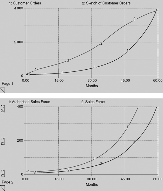
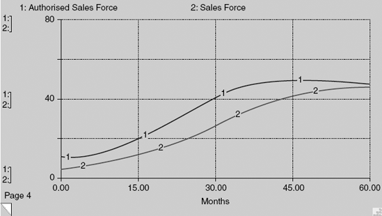
Line 1 in the bottom chart shows the authorised sales force and line 2 shows the actual sales force. In month zero, the firm employs four sales people, but already they are generating enough sales revenue to fund an authorised sales force of 10 people. This gap leads to hiring, expansion of the sales force, additional revenue, a bigger budget and a further increase in the authorised sales force. By month 30, the sales force is 41 people while the authorised force is 80, and by month 45 the sales force is 129 people while the authorised force is 248. There is continual pressure to hire and with an ever larger sales force the firm sells more and more.
Figure 7.21. Sales growth with four per cent increase in product price
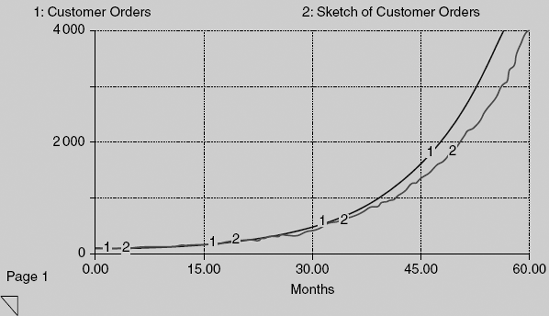
Of course no firm can grow forever, but many firms with successful products enjoy long interludes in which potential demand is far greater than realised demand. Yet even this seemingly ideal world does not always behave in quite the way one might expect. Consider, for example, the effect on sales if the product price were raised from £9 600 to £10 000, an increase of four per cent. To test this price scenario return to the model, double-click on the icon for 'product price' and enter 10000. Then go to page 1 of the graph, sketch your best guess of customer orders and press 'run'. The resulting simulation is shown in Figure 7.21. My sketch of customer orders (line 2) re-traces the trajectory of customer orders in the original simulation. So I am guessing that a four per cent price increase makes no difference to orders because we assumed, during model conceptualisation, that customers are not sensitive to price. Surprisingly, however, simulated customer orders (line 1) are higher than before. Between months 30 and 45, a clear gap opens between the two trajectories. The gap continues to grow, so that orders reach 4 000 per month in only 57 months, three months sooner than before. The reason for the sales increase lies in the reinforcing sales growth loop shown in Figure 7.14 and easily visible on-screen in the model. In this loop, product price does not directly affect the volume of customer orders. However, when price is higher, reported sales revenue is higher in the same proportion – leading to a larger budget for the sales force and eventually to a larger sales force. With higher prices, the firm can afford a larger sales force and it is this greater power of persuasion that boosts customer orders and feeds back to reinforce itself. Note the argument is dynamic – we are saying that a price increase accelerates growth in demand, not that customers prefer high prices.
Figure 7.22. Sales growth with 25 per cent increase in sales force salary
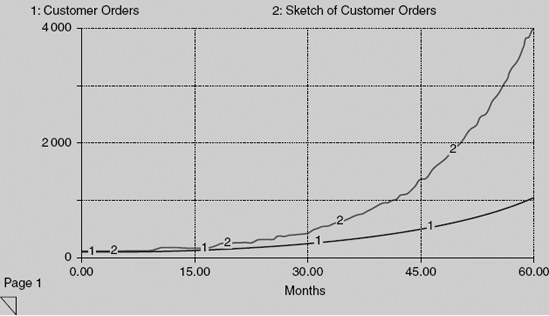
Consider another scenario in which sales force salary is increased from £4 000 to £5 000 per sales person per month, a 25 per cent increase. To test this scenario, return to the model diagram. First, modify the salary and then reset the product price to £9600. Then go to page 1 of the graph, sketch your best guess of customer orders and press 'run'. The resulting simulation is shown in Figure 7.22. Once again my sketch of customer orders follows the trajectory of the original simulation, but this time as a benchmark rather than an expectation. Simulated customer orders grow, but much more slowly than before, reaching only 1000 systems per month after 60 months rather than 4 000. Is that outcome really credible? Why should a slightly more expensive sales force do so much worse? The reason lies in a slight reduction in the strength of reinforcing feedback around the sales growth loop. The growth rate is diminished because any budget increase translates into 25 per cent fewer additional sales people and the compound effect over 60 months (five years) is huge.
7.7.2. Strength of Reinforcing Loop
The growth rate of sales depends on the strength of the reinforcing loop, which in turn depends on the economics of the sales force. If each new salesperson generates a budget surplus, a contribution to the sales budget larger than their salary, then the business will grow. If not the business will decline and the virtuous reinforcing circle will become a spiral of decline. There are four parameters around the sales growth loop that determine the budget surplus according to the following formula: budget surplus = (sales force productivity * product price * fraction of revenue to sales force) − sales force salary. Substituting numerical values from the base case model gives a budget surplus of (10 * 960 * 0.1) − 4000, which is £5 600 per sales person per month.
Further simulation experiments reveal how these factors work individually and in combination. For example, an increase in sales force productivity boosts the surplus and accelerates growth. On the other hand, as we saw above, an increase in sales force salary stunts growth. Specifically, a salary of £9600 per month reduces the budget surplus to zero and results in stagnation. More than £9 600 per month leads to decline. Intuitively, a highly paid sales force is not economic unless funded with a higher product price, a bigger slice of the budget or enhanced productivity. Any plausible combination of the four parameters that creates a healthy budget surplus leads to sustained growth. But if, for any reason, the surplus disappears then growth turns to stagnation and decline - despite the reinforcing loop and the assumption of plentiful customers.
Technically speaking a reinforcing loop generates growth when its 'steady state open-loop gain' has a value greater than one. Gain is a special measure of loop strength and is computed from the numerical values of parameters around the loop. The concept is fully explained in the Appendix of this chapter. When the steady state open-loop gain is less than one, a reinforcing loop generates a spiral of decline. When the gain is exactly equal to one then the result is stagnation. Interestingly, the gain of the sales growth loop involves the same four parameters as the budget surplus and is expressed as follows: gain = (sales force productivity * product price * fraction of revenue to sales force)/sales force salary. A gain of one corresponds to a budget surplus of zero and is the special combination of parameters in which one extra sales person contributes just enough to the sales budget to pay his or her own salary.
7.7.3. Simulation of Sales Growth and Customer Response Loops
The next partial model simulation adds the customer response loop to the sales growth loop in a scenario where production capacity is deliberately held constant. This fixed capacity is much larger than initial customer orders and so initial capacity utilisation is low and there is room for growth. Intuition suggests that in the long run fixed capacity sets a limit to growth in orders. The simulation experiment tests the intuition and shows exactly how the capacity limit is approached.
 Open the model called 'Limits to Growth in Sales' and inspect the diagram and equations. Move the pointer and hover over selected variables to check the starting conditions. The relationships include all the formulations in the previous model plus the extra policy structure and formulations for limits to sales growth presented earlier in the chapter. Note the customer response loop showing the effect of delivery delay on orders. Customer orders arrive at a rate of 35 systems per month, generated by a sales force of four people. Delivery delay recognised (by customers) is initially two months and, as a result, orders are reduced to 87 per cent of what they would otherwise be (the effect of delivery delay on orders is equal to 0.87 initially). Next, press the button labelled 'order fulfilment' to see the capacity formulations. Production capacity is 200 systems per month and the initial order backlog is 80 systems. As intended the factory is far from stretched at the start of the simulation: delivery delay minimum is only 0.4 months (80/200) and capacity utilisation is 0.2 (20 per cent) of the flat-out maximum achievable. With this modest utilisation the order fill rate is 40 systems per month (200 * 0.2), slightly greater than customer orders of 35 systems per month.
Return to sales and press the button labelled 'graph' to find a blank time chart. Before simulating, once again sketch customer orders – the trajectory you expect to see. Then press 'Run' and inspect all four pages of the graph pad. The charts in Figures 7.23 and 7.24 will appear. The top chart in Figure 7.23 shows production capacity, customer orders, and the order fill rate on a scale from zero to 400 over a period of 60 months. Note that production capacity (line 1) remains constant, as expected, at 200 systems per month throughout. Meanwhile, simulated customer orders (line 2) grow exponentially to reach the capacity limit of 200 by month 29, under the influence of the sales growth loop. Orders continue to grow for a further eight months, reaching a peak of 252 orders per month by month 37. Why is this 25 per cent overshoot possible? Surely a company cannot sell more than the factory can produce. In an equilibrium world, such an imbalance of demand and supply is impossible, but in a realistic and dynamic world, orders can exceed factory capacity for extended periods of time. Excess orders simply accumulate in backlog, leading to an increase in delivery delay, as shown in the bottom chart. Here, delivery delay indicated (line 1) begins at two months and remains steady at that value until month 18 as the factory comfortably increases capacity utilisation to accommodate growing customer orders.
Figure 7.23. Limits to sales growth with fixed capacity
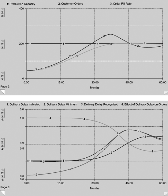
Over the next year-and-a-half to month 36 delivery delay indicated rises steadily to four months. For this entire period, customer orders (top chart, line 2) continue to rise even though customers don't want late deliveries. This apparent contradiction is explained by the lag in customers' perception of delivery delay as shown in the trajectory for delivery delay recognised (bottom chart, line 3). In the interval between months 18 and 36 the trajectory rises from two months to just less than three, even though the reality is that the factory is taking four months to deliver by month 36. Customers only gradually discover the true delivery situation. This inevitable myopia means that customers remain amenable to persuasion by the growing sales force, so orders exceed maximum capacity. By month 45, delivery delay recognised is 4 months and now customers are genuinely dissatisfied with chronic late deliveries. The sales force wins fewer orders and the growth engine is shut down and begins to go into reverse. Between months 36 and 45 customer orders fall from their peak of 250 systems per month back to 200 systems per month, in line with factory capacity. However, even this is not the end of the story. By month 45 delivery delay recognised by the customer (bottom chart, line 3) has reached just over four months and is still rising. The supply situation is highly unsatisfactory. The factory is working flat out and delivery delay indicated has reached a peak of almost six months – three times normal. Orders therefore continue to fall. Between months 45 and 60 orders remain below factory capacity. Delivery delay gradually begins to fall. The pressure on the factory eases slightly and a long-term equilibrium between orders and factory capacity begins to be established. Notice in Figure 7.24 that the sales force growth engine is neutralised. It is no longer economically attractive to hire new sales people and so market growth is halted. Technically speaking, the gain of the sales reinforcing loop has been reduced to one by permanently high delivery delay of greater than four months. In Figure 7.23 the effect of delivery delay (bottom chart, line 4) falls from 1 to 0.4, meaning that sales force productivity is slashed by 60 per cent ((1−0.4) * 100) by chronically high delivery delay.
Figure 7.24. Dynamics of sales force with fixed capacity
In reality, extreme backlog pressure on the factory would lead to capacity expansion, but our partial model shows how a capacity shortage presents itself. The effect is subtle. There is no dramatic signal to announce when the factory is overloaded. Arguably, overload is first apparent in the period between months 18 and 30 when delivery delay indicated increases from two to almost three months, but for all of that time (and bear in mind the interval is a whole year), customer orders continue to rise steadily. One could easily imagine people in the factory (and even in the sales force) concluding that customers are indifferent to delivery delay. The full consequences of late deliveries are not apparent until much later. The first clear sign is the levelling-off of customer orders in month 36, fully 18 months after the first signs of capacity shortage in the factory. The delay in the effect makes a correct attribution of the cause very difficult in practice. It is not necessarily obvious, particularly at the functional level, what corrective action is most appropriate when orders begin to falter. Should the company expand capacity or expand the sales force? Should it reduce or increase product price?
7.7.4. Simulation of the Complete Model with all Three Loops Active – The Base Case
 The complete model can shed light on these questions by probing the coordination of growth in orders, capacity and sales force. In the CD, open the model called 'Growth and Investment' and inspect the diagram and equations. The picture looks just like the previous model showing the reinforcing sales growth loop and the feedback effect of delivery delay on customer orders. Click on 'order fulfilment' to see the formulations for utilisation of capacity and order fill rate. The only visual difference by comparison with the previous model is in production capacity. The stock appears as a 'ghost' meaning that it is defined elsewhere in the model. To view the capacity formulations, first click on the 'Sales' button to return to the opening screen and then click the 'Capacity' button. Here is the policy structure for capital investment described earlier.
Move the pointer and hover over selected variables to check the starting conditions. Production capacity starts at 120 systems per month, lower than before, but comfortably more than the 35 orders per month generated by the initial sales force of four. Capacity being built is −17 systems per month at the outset. At first glance, this negative value may seem curious, but remember the capacity formulations allow for both capacity increase and decrease. If there is pressure to reduce capacity then the pipeline being built will in fact be an amount of capacity being withdrawn or temporarily idled. Pressure to change capacity stems from an assessment of delivery delay within the investment policy. In this case, delivery delay recognised by the factory is initially two months, which is the same as the delivery delay operating goal. Hence, at the start delivery delay condition takes a value of one, meaning that factory managers think the delivery situation is about right and, in their minds at least, there is no need to change capacity. However, delivery delay bias is set at 0.3 meaning that the top management team is reluctant to invest unless the evidence for expansion is really compelling. From their point of view, there is plenty of capacity and room to cut back, even though factory managers would disagree. The capacity expansion fraction takes an initial value of −0.012, calling for a modest monthly capacity reduction of just over one per cent. To be consistent, the initial pipeline of capacity being built is also negative. From these starting conditions the simulation unfolds.
Figure 7.25. Customer orders in the base case of the full model - simulated and sketched
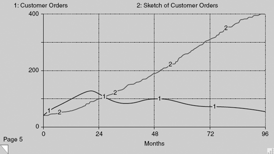
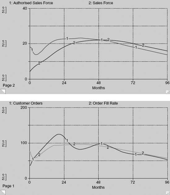
Go to the 'graph pad' and sketch customer orders you expect to see in this more complex and realistic situation with variable manufacturing capacity. Notice that the time horizon is now 96 months (eight years) to allow plenty of time to observe the pattern of market growth. Press the 'Run' button to create a time chart similar to Figure 7.25 showing sketched and simulated customer orders. In my sketch, I expect customer orders to grow slowly and steadily because I know the product is attractive and that both the sales force and capacity can be expanded to sustain growth. However, simulated orders are much different. Following a promising burst of growth to 125 systems per month in the first 20 months, orders stagnate and then decline. After 36 months, the company is selling only 80 systems per month. A turnaround then heralds a year-long recovery in which orders grow to almost 100 systems per month. But the recovery is short-lived and stagnation sets in once again at about month 48 to be followed by inexorable decline. At the end of the simulation, orders fall to merely 50 systems per month and, after eight years of trying, a once-promising market proves to be disappointingly small. Why? The remaining time charts help to explain.
Figure 7.26. Delivery delay and production capacity in the base case of the full model
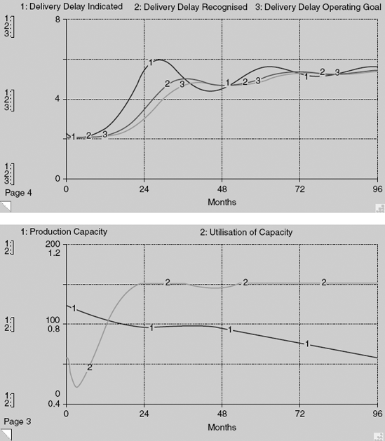
Figure 7.26 shows the behaviour over time of delivery delay and capacity. At the start of the simulation the factory is comfortably able to supply the fledgling market. Delivery delay in the top chart is two months, no matter which of the three different measures is chosen. However, during the first 28 months delivery delay indicated rises to a peak of almost six months as orders grow quickly and the factory becomes increasingly stretched. The situation in the factory is shown in the bottom chart. Utilisation of capacity (line 2) starts at a moderate 60 per cent (0.6), falls briefly and then rises quickly to its maximum value of 100 per cent (1) by month 24, where 100 per cent utilisation means the factory is working flat out, three shifts, seven days a week. In a matter of only two years the factory becomes extremely busy. Meanwhile, orders have more than trebled (Figure 7.25, line 1). So why does capacity fall? Recall that pressure to expand capacity comes from delivery delay relative to the company's operating goal. This pressure is evident in the gap between delivery delay indicated (line 1) and delivery delay operating goal (line 3) that widens for the first 28 months of the simulation. Hence, pressure to expand capacity does indeed rise as expected. The pressure is not enough, however, partly because the operating goal itself rises and partly because of the conservative investment bias of top management. Paradoxically, the company fails to expand capacity because it gets used to late deliveries.
Nevertheless, production capacity in the bottom chart does increase slightly for more than a year between months 24 and 40. However, this modest investment is not enough to reduce delivery delay back to its starting value of two months. As a result, customer orders decline and the pressure on the factory begins to subside. By month 38, delivery delay indicated is equal to the operating goal and top management is no longer convinced of the need for investment. Capacity cuts follow. The company is locked into a self-fulfilling spiral of decline. Reluctance to invest leads to high capacity utilisation and high delivery delay. Chronically high delivery delay eventually depresses customer orders and reduces the pressure to invest, thereby prolonging the capacity shortage. By the end of the simulation, delivery delay indicated (line 1) is more than five months and so too is the delivery delay operating goal (line 3). The company has inadvertently settled for long delivery times.
The consequences of dwindling capacity on the sales force and customers are shown in Figure 7.27. In the top chart, the sales force (line 2) adjusts towards the authorised sales force (line 1). The authorised force itself grows significantly in the interval between months four and 16 (fuelled by sales revenue), but later levels off and begins to decline as the product becomes more difficult to sell. By month 48, the authorised sales force is equal to the sales force and growth is halted. Thereafter, the sales force shrinks as sales people become less productive and no longer contribute enough to the sales budget to pay their own salaries. The gain of the reinforcing sales loop falls below one. Meanwhile in the bottom chart, customer orders (line 1) grow to begin with, reaching a peak of 124 systems per month in month 21. However, the order fill rate (line 2) does not keep pace with rising demand, causing an increase in delivery delay as already seen in Figure 7.26. As a result, customer orders decline sharply in the interval between months 20 and 34, even though the sales force continues to expand. There is a slight recovery when the order fill rate (line 2) briefly exceeds customer orders, thereby improving the supply situation, but eventually customer orders settle into steady decline through a combination of chronic high delivery delay and falling sales force.
Figure 7.27. Sales force, customer orders and order fill rate in the base case of the full model