
7.8. Redesign of the Investment Policy
This pattern of stagnation and decline clearly demonstrates the syndrome of growth and underinvestment mentioned at the start of the chapter. Despite huge market potential, the firm fails to achieve even modest growth. Adequate investment is simply not forthcoming. Yet the policy of capacity expansion makes sense in that it responds to realistic pressure from delivery delay. What kind of policy changes can the firm implement to dramatically improve performance and to realise the market potential?
Critics of the firm might argue it is far too inward looking. Capacity expansion relies heavily on evidence from the factory that delivery delay is too high. Surely it would be better to use a forecast of customer orders and build capacity to match. But remember, the top management team adopts a conservative attitude to investment. They listen to the evidence for expansion and discount it. More interesting than a forecast is to explore the effect of softening this conservative attitude. What if it were replaced with an optimistic attitude to approve more investment than factory managers themselves are calling for? This change calls for a fundamental shift in top management attitude to risk – a willingness to invest in capacity ahead of demand (which is rather like believing an optimistic growth forecast). We can test this change in the model by simply reversing the sign on the delivery delay bias.
7.8.1. Top Management Optimism in Capital Investment
 Return to the capacity diagram of the growth and investment model. Click on 'delivery delay bias' and change the value from 0.3 to −0.3. Review the implications of this parameter change in the equations for delivery delay pressure and capacity expansion fraction. Essentially, delivery delay pressure is higher than it would have been leading to a larger capacity expansion fraction. For example, in the case where delivery condition is one (factory managers think delivery delay is OK) then delivery delay pressure now takes a value 1.3 and top management approve capacity expansion even though factory managers do not think it is essential. Return to the graph pad and before running re-sketch customer orders (line 2) to follow the trajectory of customer orders from the base case. The sketch is now a reference for comparison. Press the 'Run' button and watch the new trajectory of customer orders unfold. The time chart at the top of Figure 7.28 appears. Notice that the number of customer orders (line 1) grows. By month 48 it reaches almost 200 systems per month by comparison with 100 systems per month in the base case. Moreover, orders continue to grow, albeit slowly, reaching 250 systems per month by the end of the simulation. The reason for this gradual growth is apparent in the bottom chart. Just as in the base case delivery delay indicated (line 1) rises as the factory tries to cope with increasing orders, but crucially this rise is less than in the base case because top management approve more investment. With extra capacity, the factory settles on a delivery delay of just over four months (rather than almost five months in the base case) and this service improvement (while far from ideal) is sufficient to sustain modest growth.
Figure 7.28. Customer orders and delivery delay with optimistic investment (sketch shows the base case)
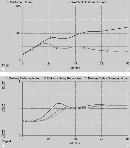
Further analysis can be carried out by investigating the other time charts showing production capacity, utilisation, sales force and authorised sales force. However, this extra work is left as an exercise for the reader. (Note that it will be necessary to re-scale the time charts in order to see the complete 96-month trajectories.) Hence, optimistic capacity expansion pays off, at least in this case. However, the resulting market growth is still far short of potential and has been bought by abandoning a belief in prudent and conservative investment. In practice, such a change of mindset may be difficult to achieve. Some would regard investment optimism as mere speculation, akin to hunch and hope.
7.8.2. High and Unyielding Standards – A Fixed Operating Goal for Delivery Delay
Pressure for capacity expansion exists whenever delivery delay exceeds the operating goal. In many organisations, however, goals drift to fit what was achieved in the past. As the goal drifts then pressure to take corrective action is reduced. But what if the goal were to remain fixed? The idea can be tested in the model by changing the delivery delay weight in the formulation for delivery delay operating goal so that all the weight goes to the management goal and none to delivery delay tradition. In practice, unyielding standards originate from the leadership whose job it is to communicate expected standards of performance and to create an environment or culture where the standards are respected and adhered to.
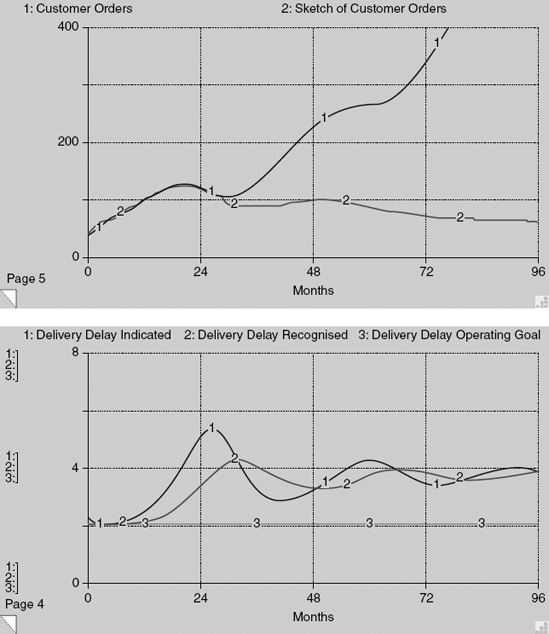
Return to the capacity diagram and click on the icon for 'delivery delay weight'. Change the weight from one to zero and then review the formulation for delivery delay operating goal to confirm that the change sets the operating goal equal to the delivery delay management goal which is itself set at two months. Make sure delivery delay bias is re-set to its original value of 0.3 (rather than −0.3). Go to page 5 of the graph pad that will show the trajectories in Figure 7.28, top chart. (If these trajectories are not showing then first re-run the experiment above to test investment optimism and then repeat the instructions in this paragraph.) Press the 'Run' button and watch the trajectory of customer orders unfold. The time chart at the top of Figure 7.29 appears. For the first 26 months customer orders (line 1) follow the base case (line 2 sketch). Thereafter orders grow quickly, reaching 225 systems per month in month 48 and 400 systems per month in month 76. This sustained growth is possible because pressure for capacity expansion remains high throughout. The bottom chart tells the story. Recall that pressure for capacity expansion is proportional to the gap between delivery delay indicated (line 1) and delivery delay operating goal (line 3). The operating goal is rock steady at two months and so when (in the initial surge of growth) delivery delay indicated rises, the gap between the two trajectories widens and stays wide. As a result much more capacity is added than in the base case, despite the reinstatement of conservative investment. Extra capacity results in lower delivery delay and so the product remains quite attractive to customers. Delivery delay recognised by the customer (line 2) settles at four months. This value is still double the operating goal, but the difference ensures continued pressure for capacity expansion to satisfy the growing volume of customer orders generated by a burgeoning sales force. With this policy change the company begins to realise the huge potential of the market.
Figure 7.29. Customer orders and delivery delay with fixed operating goal (sketch shows the base case)
Unyielding standards can unlock the market, but they are not guaranteed to work. The standards the company strives for must also be appropriate for customers. This mantra may seem obvious but it raises the question of where such standards come from. Often they are deeply held beliefs of the top management team, anchored perhaps in an intuitive understanding of the market. If the intuition is wrong then the market will not materialise. The simulator vividly shows the consequences of such a mismatch. Return to the capacity diagram and set delivery delay management goal to four months. Also check that delivery delay weight is set to zero. Return to the graph and press run. The trajectories shown in Figure 7.30 appear. In the top chart, customer orders (line 1) collapse to only three systems per month in month 24. Over the next 24 months orders stage a recovery to almost 50 systems per month but then level off and decline to end at 25 systems per month. The sketch of customer orders (line 2) re-traces the base case for comparison. Clearly a company that sets the wrong goal for delivery service performs far worse.
Figure 7.30. Customer orders and delivery delay with wrong fixed operating goal (sketch shows the base case)
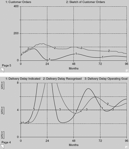
Notice the dramatic behaviour of delivery delay in the bottom chart. Delivery delay indicated (line 1) starts at two months while the operating goal (line 3) is four months. This discrepancy signals surplus production capacity that leads to disinvestment. Capacity is decommissioned and delivery delay rises sharply, going off-scale and reaching a peak value of almost 14 months after 21 simulated months. (Note that off-scale variables can be read by moving the pointer within the axes of the time chart and then clicking and holding the mouse button. A moveable vertical cursor appears. Numbers are displayed below each variable reporting their numerical values.) Delivery delay recognised by the customer (line 2) reaches a peak of 9.5 months in month 26 making it virtually impossible for the sales force to sell the product. Subsequent re-investment reduces delivery delay and revives orders, but because the delivery delay operating goal is set at four months, the amount of investment is inadequate and customer orders continue to languish.