
17.1 PRINCIPLE AND HARDWARE TOPOLOGIES
We have seen in Chapter 3, Section 3.6.1, that we can approximate a sinusoidal waveform with a staircase waveform as shown in Figure 3.21. The angular intervals for changing the waveform from a step to another and the levels for each step can be optimized by harmonic constraints. However, such dual optimization may be difficult to implement in hardware. Alternatively, levels of equal height may be easier to construct and implement within a modular approach.
Let us first imagine that each level is created with a single-phase H-bridge converter, working completely independent of the others with the only purpose of creating stair-like levels in accordance to the control strategy from Figure 17.1 (that is an extension of Figure 3.21). The base topology is shown in Figure 17.2. The operation is very intuitive as each H-bridge inverter can output one polarity or the other of the DC-side voltage by operating IGBTs on the diagonal of the H-bridge [1]. The zero voltage drop can be achieved with a zero-state in control of each module. With the decomposition shown in Figure 3.21, the conduction intervals for each IGBT can be easily depicted.
Obviously, the number of levels can be higher than three. The operation of each converter needs also to secure a constant voltage source for supply. This is assumed here as being carried out with another converter or battery not shown for simplicity.
An alternative for the converter shown in Figure 17.2 is shown in Figure 17.3, where the conventional single-phase H-bridge has been split into two inverter legs, each one contributing eventually to a different alternance of the output voltage (all three inverter legs on the left side of the figure are contributing to the positive alternance, and the three inverter legs on the right side form the negative alternance of the pole voltage). This concept is used by Siemens Corporation within High Voltage DC (HVDC) transmission lines, with multilevel converters rated up to 400 MW, and built with 200 Power Modules per Converter Arm [2].
Additional to the waveform optimization shown in Figure 17.1, another advantage of using this topology in high voltage applications is related to the ratings of the power devices. The converter leg shown in Figure 17.2 features IGBT rated for the individual DC sources, and not for the entire staircase voltage applied to the load. For instance, 1200 V IGBTs can be used in 2400 V RMS load voltage applications with the 3-level converter. The same principle applies for higher level of voltage buses. A 30 kV transmission line can thus have active filtering or voltage control within an 18-level converter, while using medium voltage IGBTs rated at 3000 V.
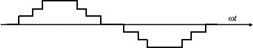
FIGURE 17.1 Multilevel waveform.
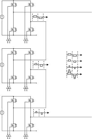
FIGURE 17.2 Three-Level converter built of three single-phase H-bridge modules.
Finally, let us note another advantage of using multilevel converters. As it will be shown later on this chapter, the PWM applied to the control of multilevel converters operates with two adjacent levels, which means that the slopes of the output voltage contain steps of smaller height. Having smaller changes in the output voltages means reduced EMI radiation produced by (dv/dt).
The modular structure of the H-Bridge multilevel converters is advantageous for manufacturing, service, and maintenance. Moreover, the high power applications allow a distributed power supply through multiple lower power DC energy sources, each being usually implemented with another power converter from a high voltage, high power AC line.
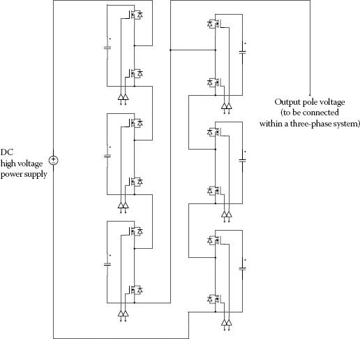
FIGURE 17.3 Another 3-level converter topology built of modules.
This approach of building multilevel converters with H-bridge modules is not very economic for multilevel converters when the power rating is relatively low. In this respect, other topologies with reduced number of components are sometimes considered.
17.1.2 FLYING CAPACITOR MULTILEVEL CONVERTER
The principle underlining this topology has been introduced in [3], and it is based on a layering structure of capacitors (Figure 17.4). Three identical legs can constitute a 3-Phase Multilevel Converter with a load connected in star. The voltage across each capacitor needs to be maintained at equal values and a capacitor voltage coincides with the voltage ratings for the power devices in converter. Moreover, the m-level flying-capacitor multilevel inverter will require m capacitors for building the m-levels in the output voltage and (m − 1) × (m − 2)/2 auxiliary capacitors per phase when the voltage rating of the capacitors is identical to that of the main switches. For instance, the particular case shown in Figure 17.4 for the 4-level converter will require 3 level-building capacitors and (4 − 1)*(4 − 2)/2 = 3 auxiliary capacitors.
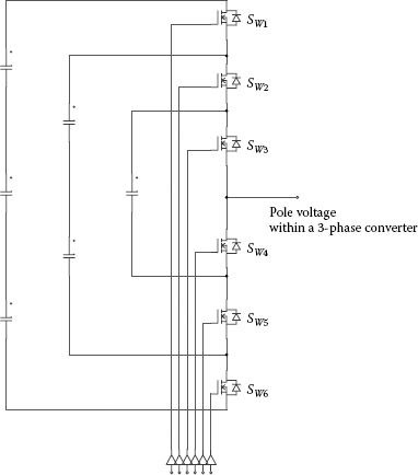
FIGURE 17.4 Flying capacitor multilevel (4-level) converter.
An important advantage of the Flying Capacitor Topology consists in its inherent redundancy. Same levels of voltage can be made up with different capacitor connection. This is illustrated within Table 17.1 true for the 4-level converter shown in Figure 17.4. This degree of freedom represents an important advantage as the voltage across the flying capacitors can be controlled by the proper selection of the switching states.
TABLE 17.1
Possible Generation of Voltage Levels in a 4-Level Flying Capacitor Converter
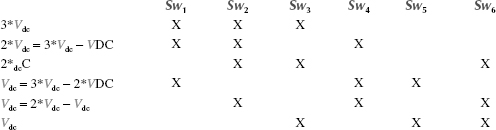
Let us also note that there are always 3 devices turned-ON for each inverter leg (phase). This can be generalized: an m-level multilevel converter has m − 1 devices (usually IGBTs) turned-ON at a given moment, on each converter leg.
The large number of capacitors amount to a large enough capacitance able to ride through short duration outages and deep voltage sags.
On the downside, the control algorithm is fairly complicated. The importance of capacitors in the proper operation of the converter is jeopardizing performance with ageing and the large capacitor value variation with temperature and ambient.
17.1.3 DIODE-CLAMPED MULTILEVEL CONVERTER
The most known and most used multilevel converter structure is shown in Figure 17.5 [4,5].
The intermediary voltage levels to be applied to the load are set-up on a capacitor divider across the high voltage DC supply voltage. The pole voltage is clamped to these intermediary voltage levels with diodes. For the case shown in Figure 17.5, the number of intermediary levels is one, and we need two capacitors to achieve this.
Similar to the previous topologies, each active switching device is required to block only a voltage level of Vdc. The multilevel converters of higher order require the clamping diodes to be chosen for different ratings, for reverse voltage blocking depending on what capacitor divider point are they connected to. Alternatively, the inverter can be designed such that each blocking diode has the same voltage rating as the active switches with n diodes in series for the diodes that need to block n × Vdc. The total number of diodes required for each pole voltage under such design yields (m − 1) × (m − 2). For instance, a 3-level converter requires 2 diodes for each pole voltage (phase).
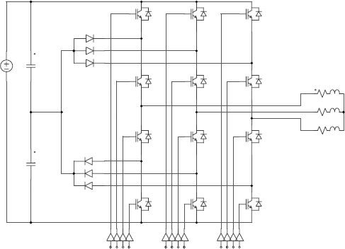
FIGURE 17.5 Diode-clamped 3-level converter.
The required amount of capacitance is lower than that of the previous topology.
The IGBTs that are turned-ON on the same inverter leg, at a given moment, are connected in series and located adjacent to each other. Moreover, the number of devices turned-ON is related to the number of levels within the inverter’s structure. For instance, a 3-level IGBT has two devices ON, a 4-level inverter has always three devices ON, and a 5-level inverter has four devices on the same leg turned ON.
The drawbacks relate to the large number of required diodes, and the somewhat difficult control algorithm for maintaining the voltage constant on the capacitors. For this reason, the use of this topology is limited to 3-level, 4-level, or 5-level converters, in a range of limited power. They were very successful in medium voltage motor drives.
A topology similar to the diode-clamped multilevel converter was presented in [6], with benefits in increasing the apparent switching frequency.
Finally, let us note that the diode-clamped inverter has redundancy in line-line voltage generation and no redundancy in phase voltage. Denoting as above the number of levels with “n,” and the instantaneous voltages on the three output waveforms as (i, j, k), the number of redundancies at a given moment yields
(17.1) |
As discussed for the H-bridge multilevel converters, these redundancies can be used for adjusting the voltages on the DC side capacitors, adjusting the neutral voltage in the output, or adjusting the sharing of the switching events between switches on the same leg.
Another design direction has been around the idea of series-connection of various converter topologies and their operation so that multilevel voltages yield on the load. This principle ranges from simple connection of two conventional bridge converters with phase shift control, to combination of any multilevel converters in order to obtain even more levels of voltages. The roots of this idea reside in multiphase transformers used with controlled rectifiers in early times of semiconductor based processing of electrical energy. We will refer to this class of converters as Combination Converters as they can emerge from a combination of any two previously shown topologies. Several examples are shown in Figure 17.6 with their appropriate waveforms [7 − 9], and this principle can be extended to a combination of any of the previously shown topologies. Note that the two DC-side power supplies do not have any common point, or—in other words—the neutral point is not connected.
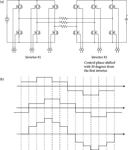
FIGURE 17.6 Simple combination multilevel converter: (a) topology; (b) principle.
17.2 DESIGN AND RATING CONSIDERATIONS
The success of multilevel converter topologies comes from the reduction of voltage seen across each power semiconductor device during operation. This means we can use these topologies in Medium and High Voltage applications with power semiconductor devices rated in a lower class. First, the medium voltage IGBTs (up to 6 kV) are the highest rated monolithic devices and the use of multilevel converters opens up the active filtering possibilities in High Voltage applications (13 kV…50 kV). On another line of thought, the switching performance, voltage drop during conduction, and cost of low voltage IGBTs (rated 1200 V) are better when compared to the medium voltage IGBTs (up to 6 kV). Hence, the use of multilevel converters benefits from lower rating IGBTs to boost the overall system level performance.
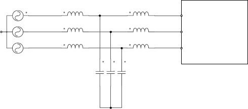
FIGURE 17.7 AC filter.
This Chapter has introduced the multilevel converters through their advantages in better approximating a sinusoidal waveform for an un-modulated operation. This helps reducing the requirements for the passive filters in AC power supplies or in grid-tied applications. This generic advantage is even more significant when PWM is used to control the power stage. Figure 17.7 shows the simplest filter structure possible. Alternatively, the trap filters can be associated to this L-C-L structure for trapping certain frequencies on the filter resonance.
It is also important to note that the operation of these filters in high-voltage applications implies the use of multiple series-connected (split) capacitors. Optimization of the way the capacitors are used within this type of connection becomes very important.
The advantages of multilevel converters are not enough exploited when PWM operation is not utilized. This can be adjusted by synthesizing intermediary voltage level in average terms (as a moving average) by spending short intervals of time in between two adjacent voltage levels. This operation mode with pulse-width modulation is well-known from the conventional bridge-like 6-switch converters.
Since we need to work with adjacent voltage levels only, the PWM algorithms are simplified and easy to understand.
Figure 17.8 explains the PWM operation of a multilevel converter with the help of conventional PWM used for varying a voltage within the DC/DC converters. The goal of an inverter is to generate a sinusoidal like voltage, and this can be achieved with multilevel converters by depicting the portion of sinusoidal waveform that belongs in between two adjacent voltage levels (level k, level k + 1), followed by the adjustment of the average pulse value in accordance to that portion of sinusoidal waveform. Furthermore, generation of PWM within a three-phase system suggests using the symmetries of a three-phase system within the PWM generation. There is a multitude of PWM algorithms reported in literature for multilevel converters and the most used methods are herein explained in detail.
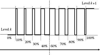
FIGURE 17.8 Principle of PWM applied to multilevel converters.
Let us first consider the generic multilevel converter shown in Figure 17.9. This structure makes abstraction of the actual converter schematic, allowing us to focus on the PWM generation algorithm without spending effort with the actual topology. Later on, we will define the particular aspects of PWM generation for each of the previously shown topologies.
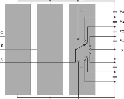
FIGURE 17.9 Schematic of an m-level 3-phase converter.
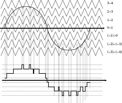
FIGURE 17.10 Sine-triangle PWM explained for a 5-level converter.
Generation of PWM voltage on each phase is illustrated in Figure 17.10 for a 4-level converter. The generic state switch from Figure 17.9 connects to the state depicted from Figure 17.10, based on the actual instantaneous position of the sinusoidal waveforms in respect to the triangular waveforms. The same algorithm is used for the other two phases with the conventional 120° phase shift. Figures 17.11, 17.12, 17.13 show the harmonic spectra when implementing this sinusoidal modulation to a 3-level converter with 10 kHz carrier modulation.
Despite the advantages of this topology with lower rating IGBT devices for a higher output voltage, the Sinusoidal PWM provides a somewhat limited output voltage. To increase the output voltage in a star-connected three-phase load, a third harmonic is injected in the reference signal.
(17.2) |
where m is the modulation index, now up to 2/sqrt(3) = 1.15.
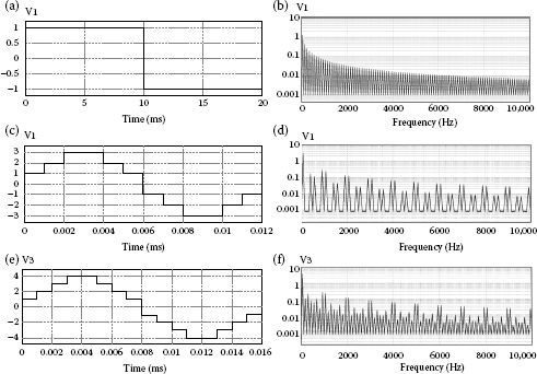
FIGURE 17.11 Harmonic spectra for un-modulated multilevel converters.
An alternative solution for the third harmonic injection, very well suited for analog implementation, is explained in [10]. The added signal is calculated from the three sinusoidal reference signals with
(17.3) |
and it can be seen as half of the distance between positive and negative envelopes of the three-phase waveforms.
If the calculation of the time intervals associated with each state is easy to be understood from Figure 17.10, the actual switching sequence is determined by properly selecting each state to provide the required voltage level.
The most common digital solution is to count the number of triangular waveforms below the reference waveform, and to enable turning-on switches on the same leg as the voltage is increasing.
At operation with a large modulation index of the diode-clamped inverter (Figure 17.12 g,h), the inner switches are switched less often than the outer switches. This shortcoming can be avoided with a proper PWM when using variable switching frequencies [11].
Advanced methods propose to improve the efficiency with
• Different frequencies for some of the carrier triangle waveforms [12];
• Shifting the boundary of the carrier triangle waveforms in order to balance the capacitor voltages [13].
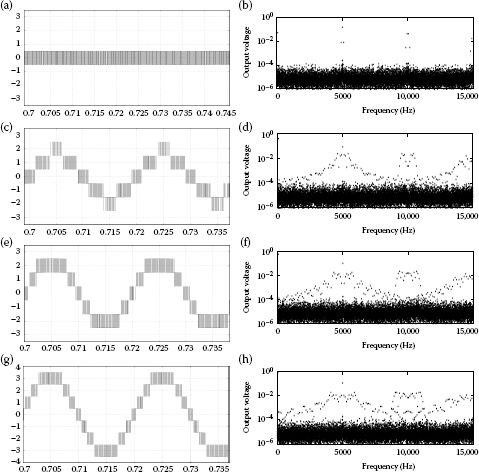
FIGURE 17.12 Harmonic spectra for sinusoidal PWM, applied to a 4-level converter with 5 kHz PWM, at different modulation indices (pole-neutral voltage shown).
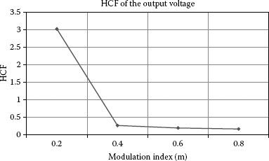
FIGURE 17.13 HCF of the output voltage in %, for the data shown on the previous figure.
17.3.3 SPACE VECTOR MODULATION
The advent in the early 1990 s of the Space Vector Modulation for conventional six-switch inverter has encouraged the use of this method to the analysis and PWM control of multilevel converters [14].
First, the possible vectorial positions within the complex plane have been identified. The multilevel converters are able to produce output voltage similar to conventional 6-switch inverters, at multiple voltage levels. For instance, the diode-clamped 3-level converter of Figure 17.5, can be operated as a conventional 2-level inverter with one capacitor voltage applied to the load through the inner IGBTs or can take advantage of switching both IGBTs on the same DC rail voltage as a series composed switch producing two times capacitor voltage on the load. This means the diagram of all available voltage space vectors will include two hexagons at 1× and 2× capacitor voltage as half of the diagonal (like radius). Moreover, the presence of all 12 switches in circuit allows some other combinations leading to other intermediary vectorial positions. A complete view on several multilevel converters is provided in Figure 17.14.
Design of a SVM method for a multilevel converter consists in identifying several vectorial locations in the neighborhood of the desired vector position, followed up by a vectorial decomposition of the desired vector into the adjacent vectorial positions. It can be observed from Figure 17.14, that any desired vectorial position will be inside a triangle formed in between three nodes. The calculation of the time intervals associated with each state is made by volt-second averaging similar to the conventional 2-level inverter.
(17.4) |
and
Decomposing the vectorial equation on the two orthogonal axes of the complex plane leads to:
(17.5) |
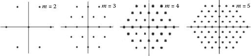
FIGURE 17.14 Vectorial positions in the complex plane of output voltage.
This system has three equations and three unknown variables, with an unique solution [ta0, tb0, tc0]. This mathematical property is very important to defining the PWM control since it also says that there is no need for zero states when controlling a multilevel converter. Since the voltage steps (fast transitions in the waveform) are smaller, it guarantees a better waveform in terms of EMI and harmonic generation.
Similar to the problem exposed in Chapter 3, Section 3.6.1, the angular intervals for changing the waveform can be calculated by optimization criteria for any of the multilevel power converters described herein (Figure 17.15). Similar to Figure 3.20, the following is explaining the principle of waveform decomposition for computer optimization. The Fourier series development helps in the calculation of harmonics through simple addition of the component waveforms.
Considering equal voltage levels, the staircase waveform of Figure 17.15(a) is decomposed in the harmonic series:
(17.6) |
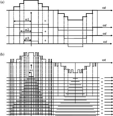
FIGURE 17.15 Decomposition in quasi-rectangular waveforms: (a) conventional staircase waveform; (b) multilevel PWM waveform.
The PWM waveform of Figure 17.15(b) is decomposed in the harmonic series:
(17.7) |
Since the calculation is very similar, we will not replicate it here [15]. Different analytical methods can be applied to solving the set of nonlinear equations derived from imposing different harmonic constraints for harmonic elimination and THD/HCF reduction. They can be implemented in mathematical programs like MathCAD.
A very interesting optimization is proposed in [16,17], where different voltage levels are considered as steps in the waveform. This allows for more degrees of freedom in harmonic optimization.
Transmission of energy on High Voltage DC lines was adopted for transmission of large amounts of energy at long distances. Examples include lines in between the United States and Quebec, or within Russia. The “classic” HVDC link works at 500 kV, under an installed power of 4000 MW [18]. Modern solutions are implemented for 800 kV lines, and a transmission power of 5000 − 7200 MW. The conventional solution consists in line-commutated power converters built of thyristors. These converters are slow in nature, yet reliable, and with a well-known operation. Recent efforts have encouraged the use of IGBT-like devices and power converters switching in the kHz range, with improved performance in the fast control of energy (more dynamics for better power quality). The drawback of this modern solution consists of additional loss in the range of 2–4% [2].
The role of a Flexible AC Transmission System is to support the proper transmission of energy. There are multiple functions implemented with power converters under this name. The most known is the Static Synchronous Compensator (STATCOM), usually implemented with Voltage Source Inverters [18]. All of these functions are used to improve the quality of the power transfer.
High voltage motor drives benefit from the multilevel converter technology with the benefits already mentioned:
• Lower ratings of the power semiconductors;
• Improved EMI radiation due to the lower steps in voltage waveform;
• Lower expectations for the input/output passive filters due to the more advantageous harmonic content when compared to conventional 6-switch bridge-like converters.
Considering these, several products have emerged on the market based on the multilevel converter technology, and are incorporating control software for motor drives applications. These target especially medium voltage, multimega-watt applications, like wind turbines, aviation power systems, and naval propulsion systems.
1. Khomfoi, S. and Tolbert, L. 2011. Chapter 31, Multilevel Power Converters, in Power Electronics Handbook, 3rd Edition. Elsevier, Butterworth-Heinemann, Amsterdam/Boston/Heidelberg/London/New York/Oxford/Paris/San Diego/San Francisco/Singapore/Sydney/Tokyo.
2. Gemmell, B., Dorn, J., Retzmann, D., and Soerangr, D. 2008. Prospects of multilevel VSC technologies for power transmission. IEEE PES Transmission and Distribution Conference and Exhibition, pp.1–16.
3. Meynard, T.A. and Foch, H. 1992. Multi-level conversion: High voltage choppers and voltage-source inverters. IEEE Power Electronics Specialists Conference, pp. 397–403.
4. Nabae, A., Takahashi, I., and Akagi, H. 1981. A new neutral-point clamped PWM inverter. IEEE Trans. Industry Appl. IA-17, 518–523.
5. Baker, R.H. 1981. Bridge Converter Circuit, U.S. Patent 4 270 163.
6. Floricau, D., Gateau, G., and Leredde, A. 2010. New active stacked NPC multilevel converter: Operation and features. IEEE Trans. Industrial Electron. 57(7), 2272–2278.
7. Corzine, K. 2005. Operation and Design of Multilevel Inverters—Report Developed for the Office of Naval Research.
8. Kawabata, T. and Ejioglu, E. 1997. New open-winding configurations for high power inverters. IEEE ISIE, pp. 457–462.
9. Stemmler, H., and Guggenbach, P. 1993. Configurations of high-power voltage source inverter drives. EPE’93, pp. 7–14.
10. Menzies, R.W., Steimer, P., and Steinke, J.K. 1994. Five-level GTO inverters for large induction motor drives. IEEE Trans. Industry Appl. 30(4), 938–944.
11. Tolbert, L.M. and Habetler, T.G. 1999. Novel multilevel inverter carrier-based PWM method. IEEE Trans. Industry Appl. 25(5), 1098–1107.
12. Tolbert, L.M. and Habetler, T.G. 1999. Novel multilevel inverter carrier-based PWM method. IEEE Trans. Industry Appl. 35(5), 1098–1107.
13. Espinoza, J., Moran, L., and Sbarbaro, D. 2003. A systematic controller design approach for neutral-point-clamped three-level inverters. Proceedings of the IEEE Industrial Electronics Conference, pp. 2191–2196.
14. Rodriguez, J., Correa, P., and Moran, L. 2001. A vector control technique for medium voltage multilevel inverters. Proceedings of the IEEE Applied Power Electronics Conference, vol. 1, pp. 173–178.
15. Chiasson, J.N., Tolbert, L.M., McKenzie, K.J., and Du, Z. 2004. A unified approach to solving the harmonic elimination equations in multilevel converters. IEEE Trans. Power Electron. 19(2), 478–490.
16. Du, Z., Tolbert, L.M., Chiasson, J.N., and Li, H. 2005. Low switching frequency active harmonic elimination in multilevel converters with unequal DC voltages. IEEE IAS Annual Meeting Conf. Rec., vol. 1, pp. 92–98, October.
17. Filho, F., Maia, H.Z., Mateus, T.H.A., Ozpineci, B., Tolbert, L.M., and Pinto, J.O.P. 2013. Adaptive selective harmonic minimization based on ANNs for cascade multilevel inverters with varying DC sources. IEEE Trans. Industrial Electron. 60(5), 1955–1962.
18. Retzmann, D. 2009. Tutorial on VSC in Transmission Systems—HVDC and FACTS, Siemens AG.