
Chapter 2
Data Structures
Understanding how data is organized within volatile storage is a critical aspect of memory analysis. Similar to files in file system analysis, data structures provide the template for interpreting the layout of the data. Data structures are the basic building blocks programmers use for implementing software and organizing how the program’s data is stored within memory. It is extremely important for you to have a basic understanding of the common data structures most frequently encountered and how those data structures are manifested within RAM. Leveraging this knowledge helps you to determine the most effective types of analysis techniques, to understand the associated limitations of those techniques, to recognize malicious data modifications, and to make inferences about previous operations that had been performed on the data. This chapter is not intended to provide an exhaustive exploration of data structures, but instead to help review concepts and terminology referred to frequently throughout the remainder of the book.
Basic Data Types
You build data structures using the basic data types that a particular programming language provides. You use the basic data types to specify how a particular set of bits is utilized within a program. By specifying a data type, the programmer dictates the set of values that can be stored and the operations that can be performed on those values. These data types are referred to as the basic or primitive data types because they are not defined in terms of other data types within that language. In some programming languages, basic data types can map directly to the native hardware data types supported by the processor architecture. It is important to emphasize that basic data types frequently vary between programming languages, and their storage sizes can change depending on the underlying hardware.
C Programming Language
This book primarily focuses on basic data types for the C programming language. Given its usefulness for systems programming and its facilities for directly managing memory allocations, C is frequently encountered when analyzing the memory-resident state of modern operating systems. Table 2-1 shows basic data types for the C programming language and their common storage sizes for both 32-bit and 64-bit architectures.
| Type | 32-Bit Storage Size (Bytes) | 64-Bit Storage Size (Bytes) |
char | 1 | 1 |
unsigned char | 1 | 1 |
signed char | 1 | 1 |
int | 4 | 4 |
unsigned int | 4 | 4 |
short | 2 | 2 |
unsigned short | 2 | 2 |
long | 4 | Windows: 4, Linux/Mac: 8 |
unsigned long | 4 | Windows: 4, Linux/Mac: 8 |
long long | 8 | 8 |
unsigned long long | 8 | 8 |
float | 4 | 4 |
double | 8 | 8 |
pointer | 4 | 8 |
The basic types in Table 2-1 are those the C standard defines. They are used extensively for the Windows, Linux, and Mac OS X kernels. Windows also defines many of its own types based on these basic types that you can see throughout the Windows header files and documentation. Table 2-2 describes several of these types.
| Type | 32-Bit Size (Bytes) | 64-Bit Size (Bytes) | Purpose/Native Type |
DWORD | 4 | 4 | Unsigned long |
HMODULE | 4 | 8 | Pointer/handle to a module |
FARPROC | 4 | 8 | Pointer to a function |
LPSTR | 4 | 8 | Pointer to a character string |
LPCWSTR | 4 | 8 | Pointer to a Unicode string |
The compiler determines the actual size of the allocated storage for the basic data types, which is often dependent on the underlying hardware. It is important to keep in mind that most of the basic data types are multiple-byte values, and the endian order also depends on the underlying hardware processing the data. The following sections demonstrate examples of how the C programming language provides mechanisms for combining basic data types to form the composite data types used to implement data structures.
Abstract Data Types
The discussion of specific data structure examples is prefaced by introducing the storage concepts in terms of abstract data types. Abstract data typesprovide models for both the data and the operations performed on the data. These models are independent of any particular programming language and are not concerned with the details of the particular data being stored.
While discussing these abstract data types, we will generically refer to the stored data as an element, which is used to represent an unspecified data type. This element could be either a basic data type or a composite data type. The values of some elements—pointers—may also be used to represent the connections between the elements. Analogous to the discussion of C pointers that store a memory address, the value of these elements is used to reference another element.
By initially discussing these concepts in terms of abstract data types, you can identify why you would use a particular data organization and how the stored data would be manipulated. Finally, we discuss examples of how the C programming language implements abstract data types as data structures and provide examples of how to use them within operating systems. You will frequently encounter implementations of data structures with which you may not be immediately familiar. By leveraging knowledge of how the program uses the data, the characteristics of how the data is stored in memory, and the conventions of the programming language, you can often recognize an abstract data-type pattern that will help give clues as to how the data can be processed.
Arrays
The simplest mechanism for aggregating data is the one-dimensional array. This is a collection of <index, element> pairs, in which the elements are of a homogeneous data type. The data type of the stored elements is then typically referred to as the array type. An important characteristic of an array is that its size is fixed when an instance of the array is created, which subsequently bounds the number of elements that can be stored. You access the elements of an array by specifying an array index that maps to an element’s position within the collection. Figure 2-1 shows an example of a one-dimensional array.
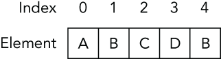
Figure 2-1: One-dimensional array example
In Figure 2-1, you have an example of an array that can hold five elements. This array is used to store characters and subsequently would be referred to as an array of characters. As a common convention you will see throughout the book, the first element of the array is found at index 0. Thus, the value of the element at index 2 is the C character. Assuming the array was given the name grades, we could also refer to this element as grades[2].
Arrays are frequently used because many programming languages offer implementations designed to be extremely efficient for accessing stored data. For example, in the C programming language the storage requirements are a fixed size, and the compiler allocates a contiguous block of memory for storing the elements of the array. You typically reference the location of the array by the memory address of the first element, which is called the array’s base address. You can then access the subsequent elements of the array as an offset from the base address. For example, assuming that an array is stored at base address X and is storing elements of size S, you can calculate the address of the element at index I using the following equation:
Address(I) = X + (I * S)
This characteristic is typically referred to as random access because the time to access an element does not depend on what element you are accessing.
Because arrays are extremely efficient for accessing data, you encounter them frequently during memory analysis. This is especially true when analyzing the operating system’s data structures. In particular, the operating system commonly stores arrays of pointers and other types of fixed-sized elements that you need to access quickly at fixed indices. For example, in Chapter 21 you learn how Linux leverages an array to store the file handles associated with a process. In this case, the array index is the file descriptor number. Also, Chapter 13 shows Microsoft’s MajorFunction table: an array of function pointers that enable an application to communicate with a driver. Each element of the array contains the address of the code (dispatch routine) that executes to satisfy an I/O request. The index for the array maps to a predefined operation code (for example, 0 = read; 1 = write; 2 = delete).
Figure 2-2 provides an example of how the function pointers for a driver’s MajorFunction table are stored in memory on an IA32-based system, assuming that the first entry is stored at base_address.
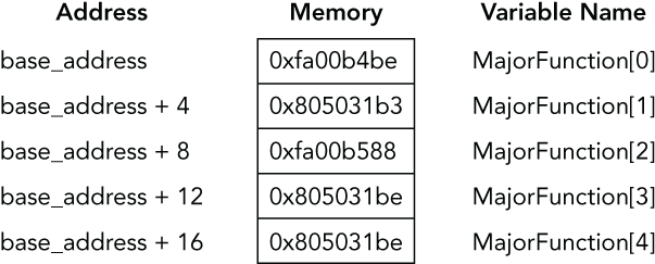
Figure 2-2: Partial array of function pointers taken from a driver’s MajorFunction table
If you know the base address of an array and the size of its elements, you can quickly enumerate the elements stored contiguously in memory. Furthermore, you can access any particular member by using the same calculations the compiler generates. You may also notice patterns in unknown contiguous blocks of memory that resemble an array, which can provide clues about how the data is being used, what is being stored, and how it can be interpreted.
Bitmaps
An array variant used to represent sets is the bitmap, also known as the bit vector or bit array. In this instance, the index represents a fixed number of contiguous integers, and the elements store a boolean value {1,0}. Within memory analysis, bitmaps are typically used to efficiently determine whether a particular object belongs to a set (that is, allocated versus free memory, low versus high priority, and so on). They are stored as an array of bits, known as a map, and each bit represents whether one object is valid or not. Using bitmaps allows for representation of eight objects in one byte, which scales well to large data sets. For example, the Windows kernel uses a bitmap to maintain allocated network ports. Network ports are represented as an unsigned short, which is 2 bytes, and provides ((216)–1) or 65535 possibilities. This large number of ports is represented by a 65535-bit (approximately 8KB) bitmap. Figure 2-3 provides an example of this Windows structure.
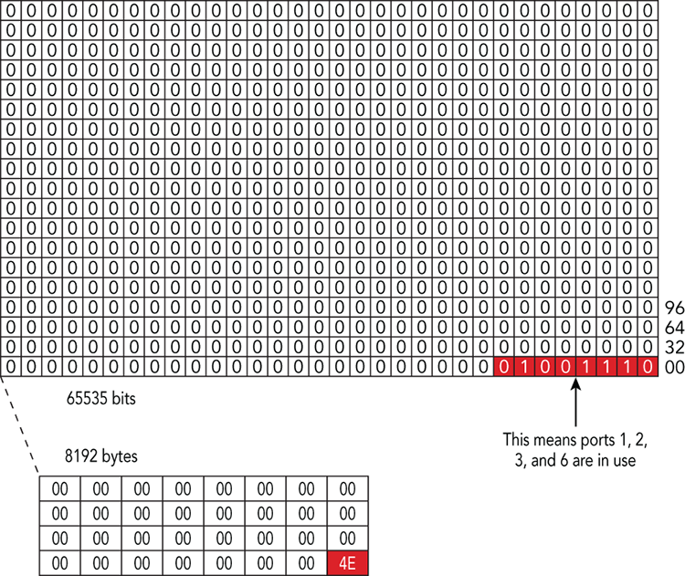
Figure 2-3: An example of a Windows bitmap of in-use network ports
The figure shows both the bit-level and byte-level view of the bitmap. In the byte-level view you can see that the first index has a value of 4e hexadecimal, which translates to 1001110 binary. This binary value indicates that ports 1, 2, 3, and 6 are in use, because those are the positions of the bits that are set.
Records
Another mechanism commonly used for aggregating data is a record (or structure) type. Unlike an array that requires elements to consist of the same data type, a record can be made up of heterogeneous elements. It is composed of a collection of fields, where each field is specified by <name, element> pairs. Each field is also commonly referred to as a member of the record. Because records are static, similar to arrays, the combination of its elements and their order are fixed when an instance of the record is created. Specifying the particular member name, which acts as a key or index, accesses the elements of a record. A collection of elements can be combined within a record to create a new element. Similarly, it is also possible for an element of a record to be an array or record itself.
Figure 2-4 shows an example of a network connection record composed of four members that describe its characteristics: id, port, addr, and hostname. Despite the fact that the members may have a variety of data types and associated sizes, by forming a record you make it possible to store and organize related objects.
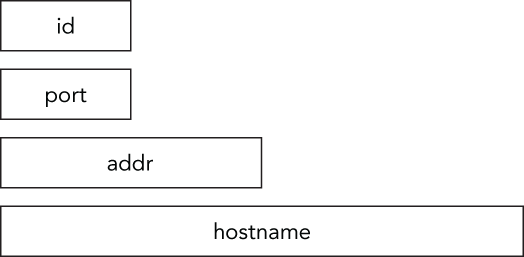
Figure 2-4: Network connection record example
In the C programming language, records are implemented using structures. A structure enables a programmer to specify the name, type, and order of the members. Similar to arrays, the size of C structures is known when an instance is created, structures are stored in a contiguous block of memory, and the elements are accessed using a base plus offset calculation. The offsets from the base of a record vary depending on the size of the data types being stored. The compiler determines the offsets for accessing an element based on the size of the data types that precede it in the structure. For example, you would express the definition of a C structure for the network connection information from Figure 2-4 in the following format:
struct Connection {
       short id;
       short port;
       unsigned long addr;
       char hostname[32];
};
As you can see, the identifier Connection is the structure’s name; and id, port, addr, and hostname are the names of its members. The first field of this structure is named id, which has a length of 2 bytes and is used to store a unique identifier associated with this record. The second field is named port, which also has a length of 2 bytes and is used to store the listening port on the remote machine. The third field is used to store the IP address of the remote machine as binary data in 4 bytes with a field name of addr. The fourth field is called hostname and stores the hostname of the remote machine using 32 bytes. Using information about the data types, the compiler can determine the proper offsets (0, 2, 4, and 8) for accessing each field. Table 2-3 lists the members of Connection and their associated offsets.
| Byte Range | Name | Type | Description |
| 0–1 | id | short | Unique record ID |
| 2–3 | port | short | Remote port |
| 4–7 | addr | unsigned long | Remote address |
| 8–39 | hostname | char[32] | Remote hostname |
The following is an example of how an instance of the data structure would appear in memory, as presented by a tool that reads raw data:
0000000: 0100 0050 ad3d de09 7777 772e 766f 6c61   ...P.>X.www.vola
0000010: 7469 6c69 7479 666f 756e 6461 7469 6f6e  tilityfoundation
0000020: 2e6f 7267 0000 0000                      .org....
C-style structures are some of the most important data structures encountered when performing memory analysis. After you have determined the base address of a particular structure, you can leverage the definition of the structure as a template for extracting and interpreting the elements of the record. One thing that you must keep in mind is that the compiler may add padding to certain fields of the structure stored in memory. The compiler does this to preserve the alignment of fields and enhance CPU performance.
As an example, we can modify the structure type from Table 2-3 to remove the port field. If the program were then recompiled with a compiler configured to align on 32-bit boundaries, we would find the following data in memory:
0000000: 0100 0000 ad3d de09 7777 772e 766f 6c61   ...P.>X.www.vola
0000010: 7469 6c69 7479 666f 756e 6461 7469 6f6e  tilityfoundation
0000020: 2e6f 7267 0000 0000                      .org....
In the output, you can see that despite removing the port field, the remaining fields (id, addr, hostname) are still found at the same offsets (0, 4, 8) as before. You will also notice that the bytes 2–3 (containing 0000), which previously stored the port value, are now used solely for padding.
As you will see in later chapters, the definition of a data structure and the constraints associated with the values that can be stored in a field can also be used as a template for carving possible instances of the structure directly from memory.
Strings
One of the most important storage concepts that you will frequently encounter is the string. The string is often considered a special case of an array, in which the stored elements are constrained to represent character codes taken from a predetermined character encoding. Similar to an array, a string is composed of a collection of <index, element> pairs. Programming languages often provide routines for string manipulation, which may change the mappings between indices and elements. While records and arrays are often treated as static data types, a string can contain a variable length sequence of elements that may not be known when an instance is created. Just as the mappings between indices and elements may change during processing, the size of the string may dynamically change as well. As a result, strings must provide a mechanism for determining the length of the stored collection.
The first implementation we are going to consider is the C-style string. C-style strings provide an implementation that is very similar to how the C programming language implements arrays. In particular, we will focus on C-style strings where the elements are of type char—a C basic data type—and are encoded using the ASCII character encoding. This encoding assigns a 7-bit numerical value (almost always stored in a full byte) to the characters in American English. The major difference between a C-style string and an array is that C-style strings implicitly maintain the string length. This is accomplished by demarcating the end of the string with an embedded string termination character. In the case of C-style strings, the termination character is the ASCII NULL symbol, which is 0x00. You can then calculate the length of the string by determining the number of characters between the string’s starting address and the termination character.
For example, consider the data structure discussed previously for storing network information whose structure type was presented in Table 2-3. The fourth element of the data structure used to store the hostname is a C-style string. Figure 2-5 shows how the string would be stored in memory using the ASCII character encoding. The string begins at byte offset 8 and continues until the termination character, 0x00, at offset 36. Thus you can determine that the string is used to store 28 symbols and the termination character.

Figure 2-5: Hostname represented in ASCII as a C-style string
You may frequently encounter an alternative string implementation when analyzing memory associated with the Microsoft Windows operating system. We will refer to this implementation as the _UNICODE_STRING implementation because that is the name of its supporting data structure. Unlike the C-style string implementation that leverages the ASCII character encoding to store 1-byte elements, the _UNICODE_STRING supports Unicode encoding by allowing elements to be larger than a single byte and, as a result, provides support for language symbols beyond just American English.
Unless otherwise specified, the elements of a _UNICODE_STRING are encoded using the UTF-16 version of Unicode. This means characters are stored as either 2- or 4-byte values. Another difference from the C-style string is that a _UNICODE_STRING does not require a terminating character but instead stores the length explicitly. As previously mentioned, a _UNICODE_STRING is implemented using a structure that stores the length, in bytes, of the string (Length), the maximum number of bytes that can be stored in this particular string (MaximumLength), and a pointer to the starting memory address in which the characters are stored (Buffer). The format of the _UNICODE_STRING data structure is given in Table 2-4.
| Byte Range | Name | Type | Description |
| 0–1 | Length | unsigned short | Current string length |
| 2–3 | MaximumLength | unsigned short | Maximum string length |
| 8–15 | Buffer | * unsigned short | String address |
Strings are an extremely important component of memory analysis, because they are used to store textual data (passwords, process names, filenames, and so on). While investigating an incident, you will commonly search for and extract relevant strings from memory. In these cases, the string elements can provide important clues as to what the data is and how it is being used. In some circumstances, you can leverage where a string is found (relative to other strings) to provide context for an unknown region of memory. For example, if you find strings related to URLs and the temporary Internet files folder, you may have found fragments of the Internet history log file.
Also important for you to understand is that the particular implementation of the strings can pose challenges, depending on the type of memory analysis being performed. For example, because C-style strings implicitly embed a terminating character that designates the end of the stored characters, strings are typically extracted by processing each character until the termination character is reached. Some challenges may arise, if the termination character cannot be found. For example, when analyzing the physical address space of a system that leverages paged virtual memory, you could encounter a string that crosses a page boundary to a page that is no longer memory resident, which would require special processing or heuristics to determine the actual size of the string.
The _UNICODE_STRING implementation can also make physical address space analysis challenging. The _UNICODE_STRING data structure only contains metadata for the string (that is, its starting virtual memory address, size in bytes, and so on). Thus, if you cannot perform virtual address translation, then you cannot locate the actual contents of the string. Likewise, if you find the contents of a string through other means, you may not be able to determine its appropriate length, because the size metadata is stored separately.
Linked Lists
A linked-list is an abstract data type commonly used for storing a collection of elements. Unlike fixed-size arrays and records, a linked-list is intended to provide a flexible structure. The structure can efficiently support dynamic updates and is unbounded with respect to the number of elements that it can store. Another major difference is that a linked-list is not indexed and is designed to provide sequential access instead of random access. A linked-list is intended to be more efficient for programs that need to frequently manipulate the stored collection by adding, removing, or rearranging elements. This added efficiency is accomplished by using links to denote relationships between elements and then updating those links as necessary. The first element of the list is commonly referred to as the head and the last element as the tail. Following the links from the head to the tail and counting the number of elements can determine the number of elements stored in a linked-list.
Singly Linked List
Figure 2-6 demonstrates an example of a singly-linked list of four elements. Each element of the singly linked list is connected by a single link to its neighbor and, as a result, the list can be traversed in only one direction. As shown in Figure 2-6, inserting new elements and deleting elements from the list requires only a couple of operations to update the links.

Figure 2-6: Singly-linked list example
To support the dynamic characteristics of linked lists and minimize storage requirements, C programming language implementations typically allocate and deallocate the memory to store elements as needed. As a result, you cannot assume that the elements will be stored contiguously in memory. Furthermore, the sequential ordering of elements is not implicit with respect to their memory location, as was the case with arrays. Instead, each element of the list is stored separately, and links are maintained to the neighboring elements. In some implementations, the links are stored embedded within the element (internal storage). In other implementations, the nodes of the linked-list contain links to the neighboring nodes and a link to the address in memory where the element is being stored (external storage). In either case, you implement the links between nodes by using pointers that hold the virtual memory address of the neighboring node. Thus, to access an arbitrary element of the list, you must traverse the linked list by following the pointers sequentially through the virtual address space.
Doubly Linked List
It is also possible to create a doubly linked list in which each element stores two pointers: one to its predecessor in the sequence and the other to its successor. Thus, you can traverse a doubly linked list both forward and backward. As you will see in the forthcoming examples, linked-list implementations can also use a variety of mechanisms for denoting the head and tail of the list.
Circular Linked List
An example linked-list implementation used frequently in the Linux kernel is the circular linked list. It is called a circular linked list because the final link stored with the tail refers to the initial node in the list (list head). This is particularly useful for lists in which the ordering is not important. A circular linked list is traversed by starting at an arbitrary list node and stopping when the list traversal returns to that node. Figure 2-7 shows an example of a circular linked list. As discussed in more detail in later chapters, this type of linked list has been used in the Linux kernel for process accounting.

Figure 2-7: Circular linked list example
Embedded Doubly Linked Lists
When analyzing process accounting for Microsoft Windows, you often encounter another linked-list implementation: an embedded doubly linked list. We refer to it as “embedded” because it leverages internal storage to embed a _LIST_ENTRY64 data structure within the element being stored. As shown in the _LIST_ENTRY64 format description in Table 2-5, the data structure contains only two members: a pointer to the successor’s embedded _LIST_ENTRY64 (Flink) and a pointer to the predecessor’s embedded _LIST_ENTRY64 (Blink). Because the links store the addresses of other embedded _LIST_ENTRY64 structures, you calculate the base address of the containing element by subtracting the offset of the embedded _LIST_ENTRY64 structure within that element. Unlike the circular linked list, this implementation uses a separate _LIST_ENTRY64 as a sentinel node, which is used only to demarcate where the list begins and ends. We discuss these and other linked-list implementations in more detail throughout the course of the book.
| Byte Range | Name | Type | Description |
| 0–7 | Flink | * _LIST_ENTRY64 | Pointer to successor |
| 8–15 | Blink | * _LIST_ENTRY64 | Pointer to predecessor |
Lists in Physical and Virtual Memory
When analyzing memory, you frequently encounter a variety of linked-list implementations. For example, you can scan the physical address space looking for data that resembles the elements stored within a particular list. Unfortunately, you cannot determine whether the data you find is actually a current member of the list from physical address space analysis alone. You cannot determine an ordering for the list, nor can you use the stored links to find neighboring elements. On the other hand, physical address space analysis does enable you to potentially find elements that may have been deleted or surreptitiously removed to thwart analysis. Dynamic data structures, such as linked lists, are a frequent target of malicious modifications because they can be easily manipulated by simply updating a few links.
In addition to physical address space analysis, you can leverage virtual memory analysis to translate the virtual address pointers and traverse the links between nodes. Using virtual memory analysis, you can quickly enumerate relationships among list elements and extract important information about list ordering.
Hash Tables
Hash tables are often used in circumstances that require efficient insertions and searches where the data being stored is in <key, element> pairs. For example, hash tables are used throughout operating systems to store information about active processes, network connections, mounted file systems, and cached files. A common implementation encountered during memory analysis involves hash tables composed of arrays of linked lists, otherwise known as chained overflow hash tables. The advantage of this implementation is that it allows the data structure to be more dynamic. A hash function, h(x), is used to convert the key into an array index, and collisions (i.e., values with the same key) are stored within the linked list associated with the hash table entry. Figure 2-8 demonstrates an example of a hash table implemented as an array of linked lists.

Figure 2-8: Hash table with chained-overflow example
In the example, searching for a particular key that results in a collision may require walking a linked list of collisions, but that is ideally much faster than walking through a list of all keys. For example, if a hash table is backed by an array of 16,000 indexes, and the hash table has 64,000 elements, an optimum hash function places 4 elements into each array index. When a search is performed, the hashed key then points to a list with only 4 elements instead of potentially traversing 64,000 elements upon each lookup.
Linux uses a chained overflow hash table (known as the process ID hash table) to associate process IDs with process structures. Chapter 21 explains how memory forensics tools leverage this hash table to find active processes.
Trees
A tree is another dynamic storage concept that you may encounter when analyzing memory. Although arrays, records, strings, and linked lists provide convenient mechanisms for representing the sequential organization of data, a tree provides a more structured organization of data in memory. This added organization can be leveraged to dramatically increase the efficiency of operations performed on the stored data. As shown in later chapters, trees are used in operating systems when performance is critical. This section introduces basic terminology and concepts associated with hierarchical (rooted) trees, the class of trees most frequently encountered when analyzing memory.
Hierarchical Trees
Hierarchical trees are typically discussed in terms of family or genealogical trees. A hierarchical tree is composed of a set of nodes used to store elements and a set of links used to connect the nodes. Each node also has a key used for ordering the nodes. In the case of a hierarchical tree, one node is demarcated as the root, and the links between nodes represent the hierarchical structure through parent-child relationships. Links are used to connect a node (parent) to its children. As an example, a binary tree is a hierarchical tree in which each node is limited to no more than two children. A node that does not have any children (proper descendants) is referred to as a leaf. The only non-leaf (internal node) without a parent is the root. Any node in the tree and all its descendants form a subtree. A sequence of links that are combined to connect two nodes of the tree is referred to as a path between those nodes. A fundamental property of a hierarchical tree is that it does not possess any cycles. As a result, a unique path exists between any two nodes found in the tree. Figure 2-9 shows a simplified representation of a tree.

Figure 2-9: A tree containing six nodes
Figure 2-9 is an example of a binary tree containing six nodes that are used to store integers. In the case of binary trees, the links associated with each node are referred to as the left and right link, respectively. For the sake of simplicity, the key corresponds with the integer being stored, and each node is referenced using the key. The root of the tree is node 4; nodes 2 and 4 are internal nodes; and the leaf nodes are 1, 3, and 5. Combining the sequence of links between nodes 4, 2, and 3 is used to form the unique path from node 4 to node 3. Node 2 and its descendants, nodes 1 and 3, would be considered a subtree rooted at 2.
Tree Traversal
One of the most important operations to be performed on a tree, especially during memory analysis, is tree traversal, which is the process of visiting the nodes of a tree to extract a systematic ordering. Unlike the linked list abstract data type in which you traverse nodes by following the link to its neighbor, each node of a tree can potentially maintain links to multiple children. Thus an ordering is used to determine how the edges to the children should be processed. The different techniques are classified based on the order in which the nodes are visited. The three most frequently encountered orderings are preorder, inorder, and postorder. Each of the following descriptions is performed recursively at each node encountered. Using preorder traversal, you first visit the current node and then visit the subtrees from left to right. Inorder traversal involves visiting the left subtree, then the current node, and finally the remaining subtrees from left to right. During postorder traversal, you visit each subtree from left to right and then visit the current node. The following shows the preorder, inorder, and postorder orderings of the nodes.
___________________________

Preorder:  4, 2, 1, 3, 6, 5
Inorder:   1, 2, 3, 4, 5, 6
Postorder: 1, 3, 2, 5, 6, 4
___________________________
C-programming implementations of trees have many of the same characteristics as linked lists. The major differences are the number and types of links maintained between nodes and how those links are ordered. As in the linked list implementations, we will focus on trees in which the memory for the nodes of the tree is dynamically allocated and deallocated as needed. We will also primarily focus on explicit implementations that use internal storage to embed the links within the stored elements. These links are implemented as direct edges in which each node maintains pointers to the virtual memory addresses of related nodes.
Analyzing Trees in Memory
Analyzing trees in memory also shares similar challenges faced during the analysis of linked lists. For example, physical memory analysis offers the potential to find instances of stored or previously stored elements scattered throughout memory, but does not have the context to discern relationships between those elements. On the other hand, you can leverage virtual memory analysis to traverse the tree to extract node relationships and stored elements. In the case of an ordered tree, if you know the traversal order or can discern it from the field names, you can extract the ordered list of elements. By combining the overall structure of the tree with the ordering criteria, you may even be able to discern information about how the elements were inserted or removed from the tree as it evolved over time.
This book highlights many different variants of trees and how they are used within operating systems. For example, the Windows memory manager uses a virtual address descriptor (VAD) tree to provide efficient lookups of the memory ranges used by a process. The VAD tree is an example of a self-balancing binary tree that uses the memory address range as the key. Intuitively, this means that nodes containing lower memory address ranges are found in a node’s left subtree, and nodes containing higher ranges are found in the right subtree. As you will see in Chapter 7, using these pointers and an inorder traversal method, you can extract an ordered list of the memory ranges that describes the status of the process’s virtual address space.
Summary
Data structures play a critical role in memory analysis. At the most fundamental level, they help us make sense of the otherwise arbitrary bytes in a physical memory dump. By understanding relationships among the data (i.e., nodes within a tree, elements of a list, characters of a string), you can begin to build a more accurate and complete representation of the evidence. Furthermore, knowledge of an operating system’s specific implementation of an abstract data structure is paramount to learning why certain attacks (that manipulate the structure(s)) are successful and how memory analysis tools can help you detect such attacks.