7. Multiple Regression in Marketing-Mix Models

The A’s know most major-league teams use batting average (hits over real opportunities) as the prevailing metric for determining the worth of a hitter. Traditional wisdom says, “You hit more, you win more.” So the players who have more hits per at bat¹ are generally the most sought after and are paid the most money. But by examining the outcome of decades of baseball games, the A’s find a variable they believe to be more predictive of success. It is not only hits that help a baseball team win; walks count too. Getting on base and not making outs is more closely correlated with winning games than hits alone.

The team’s management takes the analysis of the data and uses it to buy undervalued players—players who don’t necessarily have the highest batting averages but who do have high on-base percentages. For a small-market team such as the A’s, which has less money to spend on players than other franchises, this strategy changes the game.

Moneyball is about baseball, but the idea also works in the context of business marketing. Although management often makes assumptions, by actually analyzing the data, a business can better understand how to succeed. And if a business can find an important variable before others begin using it, management can build its strategy around that variable to gain an advantage.

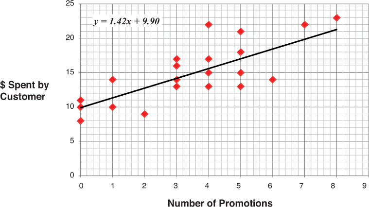
Consider the following common marketing-mix example for a hypothetical company, No More Germs, which sells toothpaste. To determine the relationship between the number of promotions the company does and the number of units it sells, the company plots its known data on an x–y plane (Figure 7-1). On the x-axis, the company plots the number of promotions (such as price reductions) it could have in a month. On the y-axis, No More Germs plots the number of purchases made by customers for each level of promotions.

Source: All figures created by case writer unless otherwise specified.

Figure 7-1 Illustration of single-variable regression

In this example, No More Germs has data covering a time period of 29 weeks, promotions ranging between 0 and 9, and corresponding sales from 10 to 23. A linear, single-variable regression analysis can be run on this data with the aid of computer software.² The results will help No More Germs examine the relationship between the number of promotions and the number of sales to customers by producing a function that describes the relationship. The objective is to draw a line that at each point represents the number of sales that are likely for any given number of promotions. In this case, the x variable—or independent variable—is the number of promotions. The y variable—or dependent variable (known as such because it depends on x)—is units sold.

The function produced by the regression is intended to cover as many of the known data points as possible and/or reduce the distance between the line and the points as much as possible. This allows the data analyst to accurately predict sales that are likely, given the number of promotions in other sample sets of data (in this case, if data from other weeks is used). The equation from the regression analysis for the best-fit straight line for No More Germs is y = 1.42x + 9.9.

The most critical outputs of the regression for the marketing manager are two coefficients: the intercept (9.9) and the slope (1.42) of the line. The intercept represents the number of sales that are likely when promotions are 0, which is equal to 9.9 in this example. This is the point where the line crosses the y-axis. The slope of the line describes the relationship between sales (y, or the dependent variable) and promotions (x, or the independent variable) by stating the ratio of the change in y to a unit change in x. In the example, the number of sales changes 1.42 per one-unit increase in promotions (Figure 7-2). The slope (often referred to as “rise over run”) is, therefore, 1.42 ÷ 1, or 1.42.

Figure 7-2 Illustration of slope in a single-variable regression

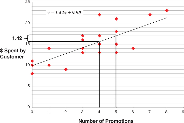
Three things can be determined immediately by looking at the slope of the line: (1) If the number is positive, the relationship between the two variables is positive, meaning as the independent variable increases, so does the dependent variable; (2) if the slope of the line is 0, no changes are observed in the dependent variable as the independent variable changes (in other words, the variables are not correlated); and (3) if the slope of the line is negative, a change in the independent variable will produce the opposite effect in the dependent variable (in this case, No More Germs’ sales would decrease if promotions increased).

Remember that although in this case the relationship between promotions and sales is obvious, in most cases a regression analysis is used to show a relationship between variables that are not as clearly related. For example, what if No More Germs wanted to know what kind of effect web advertising had on sales of its products? The company’s marketing manager might not know how effective web ads are compared with print ads, for example, and the regression would assist him or her in deciding where to put the company’s advertising dollars.

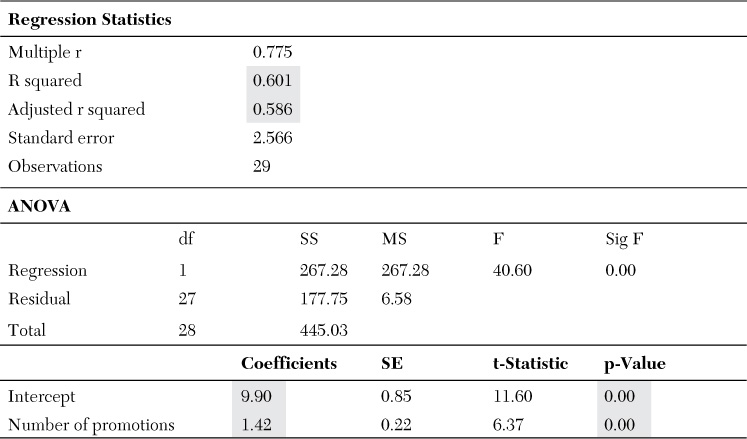
The output of No More Germs’ sample regression (which is typical of these reports) is shown in Table 7-1. Although the analysis yields multiple statistics, the most critical for marketing analysts (in addition to the coefficients of the equation) are r squared and p-value. In this example, r squared is 60%, meaning the line described by this function is appropriate for explaining 60% of the data points. This indicates how accurate the function is within the current sample of data. (Note: A typical marketing-focused regression would have an r squared of about 20% to 30%, as there are numerous factors that affect sales—such as competition, weather, and so on—that would be unknown before running the analysis.)

Table 7-1 Illustration of Output from Single-Variable Regression Analysis

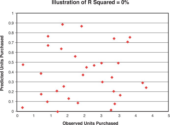
To better understand the meaning of r squared, imagine your regression output indicates an r squared of 0. The resulting plot will look like a disorderly circle of data (Figure 7-3).

Figure 7-3 Illustration of r squared = 0%

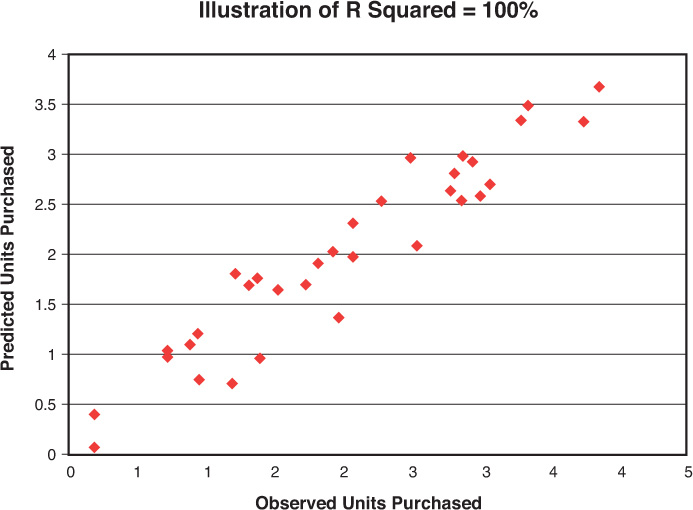
A line cannot be produced that will explain any of the data. Now imagine r squared is 100%. In this case, all of the data points (dots) will be on a line (Figure 7-4). The line accounts for all of the points in the data set. All regression analyses will result in lines with accuracy somewhere in between these extremes.

Figure 7-4 Illustration of r squared = 100%

P-value describes the significance of the findings given the sample size. But what does significant mean? In this population sample, 29 observations are made. Because this is a regression analysis of a small sample, you want to know whether you will still see the resulting coefficients if you include another 29 observations or another 29,000 observations. Will the slope of the line be 1.42, or will it be 0 or negative? Here, the p-value indicates there is a 0% chance the coefficients will change beyond the standard error given the addition of more data points or different samples. Most important, it indicates a 0% chance the slope will become negative, indicating the opposite relationship between the variables than what is indicated by the regression. In other words, regardless of how many times the data is sampled, the relationship will hold.

In addition to these critical outputs of a regression analysis, it might be beneficial to be familiar with one other value. In this example, t-stat is a reflection of p-value; however, depending on the regression or model used, the name of this value may change (for example, chi-square). P-value, on the other hand, will always be referred to in the same way. Particularly for marketing managers, who in most cases will need to be smart consumers of regression outputs but will not have to run the analyses themselves, p-value will provide adequate information about the significance of the findings.

The data shown in Table 7-2 reflects an analysis of three variables: price paid, whether the unit was on feature (highlighted in a mailer or other promotion but not necessarily at a reduced price), and whether the unit was on a store display (on an endcap or stand-alone cardboard cutout). In this case, you know the true effect of each of these variables on the outcome because you created the model. This is evidenced by the fact that you have an r squared of 99% (with the 1% error inserted randomly in the true model you created).

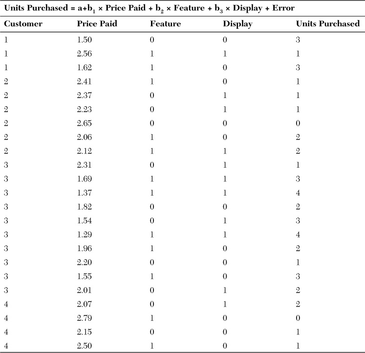
Feature and Display:

1 = Yes

0 = No

Table 7-2 Hypothetical Data on Sales of No More Germs Toothpaste

Because this is a hypothetical situation, the data is known to coincide with the true model (Table 7-3), in which the intercept is 6.22, the price coefficient is –2.28 (meaning the slope is downward and, as price increases, sales decrease), the feature coefficient is 0.38, and the display coefficient is 0.22 (meaning the slope is upward and, as feature and display increase, sales increase). Also, because this is the true model, r squared is 0.99, indicating an extremely low chance of error.

Table 7-3 Model Estimates Using Hypothetical Data

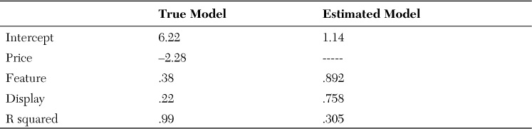
But imagine you are a marketing manager, and you don’t have access to the true model. (In fact, no one can know the true model in any real-world situation.) Looking only at the data, you must approximate the true model as closely as possible. Imagine now that you don’t think price is important in your model, and consider only feature and display. As shown in Table 7-3, the resulting coefficients describing the effect those variables have on units purchased are higher than in the true model.

Because you would not have access to the true model in a real-world situation, what would these results influence you as a manager to do? You would expect that feature and display would be more effective than they in fact are and invest more heavily in those marketing strategies. As shown in the true model, however, price has a great effect on units purchased, and the effects of feature and display are therefore overstated in the estimated model.

To correct such a bias, intuition comes into play. First, a good marketing manager should know from experience that price has a significant effect on units purchased. A good marketing manager should also know that when items are on feature and display, they tend to come with a reduced price. In other words, price and feature/display tend to be negatively correlated.

This is what is known as an omitted-variable bias because the estimated model has not taken into account a variable that has a significant effect on what is being measured. Although such biases may not always be as obvious as in this example, they are common in multivariable regression analyses, and this is the main point of differentiation when moving away from single-variable analyses (which are, by nature, oversimplified and, at least in terms of marketing, fail to fully explain most real-world situations).

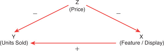
To ensure a bias is not detrimental to the findings of a regression analysis, you must examine the direction of the bias. In this case, the bias is positive because feature and display have a higher coefficient in the estimated model than in the true model. But how do you know the direction of the bias if you do not know the true model? Again, some intuition and experience are necessary. You know price and sales have a negative correlation. You know price and feature and price and display also have a negative correlation. The direction of the bias when price is the omitted variable is the product of the sign of the correlation between price and units purchased and the sign of the correlation between price and feature and display. The product of a negative and a negative is a positive, so in this case, the bias is positive (Table 7-4).

Table 7-4 Correlation Between Independent and Dependent Variables

Another way to think about omitted variables is shown in Figure 7-5. Here, x and y are shown with respect to some omitted variable, z. By examining this relationship, the marketing manager can determine the direction of the bias created by omitting that variable.

Figure 7-5 Illustration of omitted variable bias

Note that an omitted variable is only a problem when it affects both whatever is included in the model and the dependent variable. If it is not correlated with other independent variables in the model, removing it will reduce r squared, but it will not affect the coefficient of the variables included in the model. In the current example, the variation in units is being assigned to feature and display, when in fact it should be assigned to price. If the changes in one variable did not affect another, whatever variation in the dependent variable was being captured would still reflect reality. For example, weather can have a profound effect on sales (for example, a hurricane keeping buyers in Florida from making it to stores for an extended period), but hurricanes need not necessarily affect the feature or display plans for a brand. If weather and feature and display plans are not correlated, then inclusion of weather is not necessary to obtain accurate estimates of feature or display.

In this example, you have what is known as an optimistic model, which can be a concern for marketing managers. When presenting such results to decision makers, the findings will be overstated because a significant variable (price) was omitted. Although you cannot include everything in your model, knowing whether the results are conservative or optimistic is beneficial. Typically, a conservative model (one that has a negative bias) is best. Investing in a marketing channel shown to be effective by a conservative model may still represent lost opportunity if the amount of the investment is low, but it will not represent an outright mistake in resource allocation.

When do you know if you have the true model? You never know, but examining the four Ps (product, price, place, and promotion) is a good place to start. The results of a regression analysis are only hypotheses, and they should be tested in field experiments to ensure their validity.

But how do you know when it makes economic sense to invest in the findings of a regression? As a marketing manager, you must ask yourself if the benefit of a marketing intervention (such as the size of the coefficient) justifies the expense. This is what is known as economic significance.

Consider the single-variable-regression example in which you examined promotions versus purchases. The benefit provided from one promotion was found to be an increase in number of sales of 1.42. This was found to be a statistically significant finding. To determine economic significance, you must weigh this benefit against the cost of doing a promotion, taking into account the gross profit from the sale of a single unit.

Assume that the gross profit per unit is $5 and the cost of a promotion is $0.50. Therefore, profit = (units purchased × gross profit) – (cost of promotion × number of promotions), or:

Profit = 1.42 × 5 – 0.50 × 1 = 7.1 – 0.5 = 6.6

In this example, the company will make $6.60 per promotion. But if the cost of the promotion increases or the company makes less gross profit per unit, the economic significance of the promotion could quickly be lost. In other words, even if your regression findings are significant, you must first use a profit/loss function before taking action.

The value of a regression model is only as good as the variables selected to be in the model. Strong managerial intuition is required to identify variables (such as price, feature, and display, among others) that are most closely related to sales. For the best results, managers should also have some insight into how these variables actually relate in the real world to determine whether the results of a regression might be conservative or overly optimistic. This intuition is the artistic or creative side of analytics and is necessary to move a regression beyond a statistical exercise and turn it into something valuable for a business.

2. For more information on how to perform a regression using computer software, please visit Darden Marketing Analytics at http://dmanalytics.org/.