
CHAPTER
SIX
BOND PRICING, YIELD MEASURES, AND TOTAL RETURN
FRANK J. FABOZZI, PH.D., CFA, CPA
Professor of Finance
EDHEC Business School
In this chapter the pricing of fixed income securities and the various measures of computing return (or yield) from holding a fixed income security will be explained and illustrated. The chapter is organized as follows: In the first section, we apply the present-value analysis to explain how a bond’s price is determined. Then we turn to yield measures, first focusing on conventional yield measures for a fixed-rate bond (yield-to-maturity and yield-to-call in the case of a callable bond) and a floating-rate bond. After highlighting the deficiencies of the conventional yield measures, a better measure of return—total return—is then presented.
BOND PRICING
The price of any financial instrument is equal to the present value of the expected cash-flow. The interest rate or discount rate used to compute the present value depends on the yield offered on comparable securities in the market. In this chapter we shall explain how to compute the price of an option-free bond (i.e, a bond that is not callable, putable, or convertible). The pricing of bonds with embedded options is explained in Chapter 40.
Determining the Cash-Flow
The first step in determining the price of a bond is to determine its cash-flow. The cash-flow of an option-free bond consists of (1) periodic coupon interest payments to the maturity date and (2) the par (or maturity) value at maturity. Although the periodic coupon payments can be made over any time interval (weekly, monthly, quarterly, semiannually, or annually), most bonds issued in the United States pay coupon interest semiannually. In our illustrations, we shall assume that the coupon interest is paid semiannually. Also, to simplify the analysis, we shall assume that the next coupon payment for the bond will be made exactly six months from now. Later in this section we explain how to price a bond when the next coupon payment is less than six months from now.
In practice, determining the cash-flow of a bond is not simple, even if we ignore the possibility of default. The only case in which the cash-flow is known with certainty is for fixed-rate, option-free bonds. For callable bonds, the cash-flow depends on whether the issuer elects to call the issue. In the case of a putable bond, it depends on whether the bondholder elects to put the issue. In either case, the date that the option will be exercised is not known. Thus the cash-flow is uncertain. For mortgage-backed and asset-backed securities, the cash-flow depends on prepayments. The amount and timing of future prepayments are not known, and therefore, the cash-flow is uncertain. When the coupon rate is floating rather than fixed, the cash-flow depends on the future value of the reference rate. The techniques discussed in Part 5 have been developed to cope with the uncertainty of cash-flows. In this chapter, the basic elements of bond pricing where the cash-flow is assumed to be known are presented.
The cash-flow for an option-free bond consists of an annuity (i.e., the fixed coupon interest paid every 6 months) and the par or maturity value. For example, a 20-year bond with a 9% (4.5% per 6 months) coupon rate and a par or maturity value of $1,000 has the following cash-flows:
Semiannual coupon interest = $1,000 × 0.045
= $45
Maturity value = $1,000
Therefore, there are 40 semiannual cash-flows of $45, and a $1,000 cash-flow 40 six-month periods from now.
Notice the treatment of the par value. It is not treated as if it will be received 20 years from now. Instead, it is treated on a consistent basis with the coupon payments, which are semiannual.
Determining the Required Yield
The interest rate that an investor wants from investing in a bond is called the required yield. The required yield is determined by investigating the yields offered on comparable bonds in the market. By comparable, we mean option-free bonds of the same credit quality and the same maturity.1
The required yield typically is specified as an annual interest rate. When the cash-flows are semiannual, the convention is to use one-half the annual interest rate as the periodic interest rate with which to discount the cash-flows. A periodic interest rate that is one-half the annual yield will produce an effective annual yield that is greater than the annual interest rate.
Although one yield is used to calculate the present value of all cash-flows, there are theoretical arguments for using a different yield to discount the cash-flow for each period. Essentially, the theoretical argument is that each cash-flow can be viewed as a zero-coupon bond, and therefore, the cash-flow of a bond can be viewed as a package of zero-coupon bonds. The appropriate yield for each cash-flow then would be based on the theoretical rate on a zero-coupon bond with a maturity equal to the time that the cash-flow will be received. For purposes of this chapter, however, we shall use only one yield to discount all cash-flows. In later chapters, this issue is reexamined.
Determining the Price
Given the cash-flows of a bond and the required yield, we have all the necessary data to price the bond. The price of a bond is equal to the present value of the cash-flows, and it can be determined by adding (1) the present value of the semiannual coupon payments and (2) the present value of the par or maturity value.
Because the semiannual coupon payments are equivalent to an ordinary annuity, the present value of the coupon payments and maturity value can be calculated from the following formula:2
where
c = semiannual coupon payment ($)
n = number of periods (number of years times 2)
i = periodic interest rate (required yield divided by 2) (in decimal)
M = maturity value
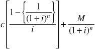
Illustration 1. Compute the price of a 9% coupon bond with 20 years to maturity and a par value of $1,000 if the required yield is 12%.
The cash-flows for this bond are as follows: (1) 40 semiannual coupon payments of $45 and (2) $1,000 40 six-month periods from now. The semiannual or periodic interest rate is 6%.
The present value of the 40 semiannual coupon payments of $45 discounted at 6% is $677.08, as shown below:
The present value of the par or maturity value 40 six-month periods from now discounted at 6% is $97.22, as shown below:
The price of the bond is then equal to the sum of the two present values:
Illustration 2. Compute the price of the bond in Illustration 1 assuming that the required yield is 7%.
The cash-flows are unchanged, but the periodic interest rate is now 3.5% (7%/2).
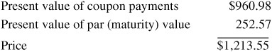
The present value of the 40 semiannual coupon payments of $45 discounted at 3.5% is $960.98, as shown below:
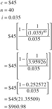
The present value of the par or maturity value of $1,000 40 six-month periods from now discounted at 3.5% is $252.57, as shown below:

The price of the bond is then equal to the sum of the two present values:
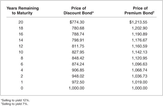
Relationship between Required Yield and Price at a Given Time
The price of an option-free bond changes in the direction opposite to the change in the required yield. The reason is that the price of the bond is the present value of the cash-flows. As the required yield increases, the present value of the cash-flows decreases; hence the price decreases. The opposite is true when the required yield decreases: The present value of the cash-flows increases, and therefore, the price of the bond increases.
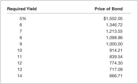
We can see this by comparing the price of the 20-year, 9% coupon bond that we priced in Illustrations 1 and 2. When the required yield is 12%, the price of the bond is $774.30. If, instead, the required yield is 7%, the price of the bond is $1,213.55. Exhibit 6–1 shows the price of the 20-year, 9% coupon bond for required yields from 5% to 14%.
EXHIBIT 6–1
Price/Yield Relationship for a 20-Year, 9% Coupon Bond
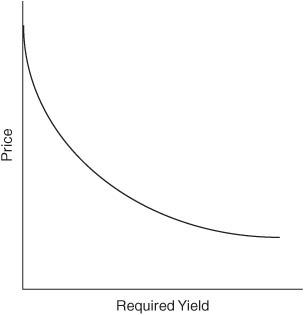
If we graphed the price/yield relationship for any option-free bond, we would find that it has the “bowed” shape shown in Exhibit 6–2. This shape is referred to as convex.3 The convexity of the price/yield relationship has important implications for the investment properties of a bond. We’ve devoted Chapter 7 to examining this relationship more closely.
EXHIBIT 6–2
Price/Yield Relationship
The Relationship among Coupon Rate, Required Yield, and Price
For a bond issue at a given point in time, the coupon rate and the term-to-maturity are fixed. Consequently, as yields in the marketplace change, the only variable that an investor can change to compensate for the new yield required in the market is the price of the bond. As we saw in the preceding section, as the required yield increases (decreases), the price of the bond decreases (increases).
Generally, when a bond is issued, the coupon rate is set at approximately the prevailing yield in the market.4 The price of the bond then will be approximately equal to its par value. For example, in Exhibit 6–1, we see that when the required yield is equal to the coupon rate, the price of the bond is its par value. Consequently, we have the following properties:
When the coupon rate equals the required yield, the price equals the par value.
When the price equals the par value, the coupon rate equals the required yield.
When yields in the marketplace rise above the coupon rate at a given time, the price of the bond has to adjust so that the investor can realize some additional interest. This adjustment is accomplished by having the bond’s price fall below the par value. The difference between the par value and the price is a capital gain and represents a form of interest to the investor to compensate for the coupon rate being lower than the required yield. When a bond sells below its par value, it is said to be selling at a discount. We can see this in Exhibit 6–1. When the required yield is greater than the coupon rate of 9%, the price of the bond is always less than the par value. Consequently, we have the following properties:
When the coupon rate is less than the required yield, the price is less than the par value.
When the price is less than the par value, the coupon rate is less than the required yield.
Finally, when the required yield in the market is below the coupon rate, the price of the bond must be above its par value. This occurs because investors who could purchase the bond at par would be getting a coupon rate in excess of what the market requires. As a result, investors would bid up the price of the bond because its yield is attractive. It will be bid up to a price that offers the required yield in the market. A bond whose price is above its par value is said to be selling at a premium. Exhibit 6–1 shows that for a required yield less than the coupon rate of 9%, the price of the bond is greater than its par value. Consequently, we have the following properties:
When the coupon rate is greater than the required yield, the price is greater than the par value.
When the price is greater than the par value, the coupon rate is greater than the required yield.
Time Path of a Bond
If the required yield is unchanged between the time the bond is purchased and the maturity date, what will happen to the price of the bond? For a bond selling at par value, the coupon rate is equal to the required yield. As the bond moves closer to maturity, the bond will continue to sell at par value. Thus, for a bond selling at par, its price will remain at par as the bond moves toward the maturity date.
The price of a bond will not remain constant for a bond selling at a premium or a discount. For all discount bonds, the following is true: As the bond moves toward maturity, its price will increase if the required yield does not change. This can be seen in Exhibit 6–3, which shows the price of the 20-year, 9% coupon bond as it moves toward maturity, assuming that the required yield remains at 12%. For a bond selling at a premium, the price of the bond declines as it moves toward maturity. This can also be seen in Exhibit 6–3, which shows the time path of the 20-year, 9% coupon bond selling to yield 7%.
EXHIBIT 6–3
Time Paths of 20-Year, 9% Coupon Discount and Premium Bonds
Reasons for the Change in the Price of a Bond
The price of a bond will change because of one or more of the following reasons:
• A change in the level of interest rates in the economy. For example, if interest rates in the economy increase (fall) because of Fed policy, the price of a bond will decrease (increase).
• A change in the price of the bond selling at a price other than par as it moves toward maturity without any change in the required yield. As we demonstrated, over time a discount bond’s price increases if yields do not change; a premium bond’s price declines over time if yields do not change.
• For non-Treasury bonds, a change in the required yield due to changes in the spread to Treasuries. If the Treasury rate does not change but the spread to Treasuries changes (narrows or widens), non-Treasury bond prices will change.
• A change in the perceived credit quality of the issuer. Assuming that interest rates in the economy and yield spreads between non-Treasuries and Treasuries do not change, the price of a non-Treasury bond will increase (decrease) if its perceived credit quality has improved (deteriorated).
• For bonds with embedded options (callable bonds, putable bonds, and convertible bonds), the price of the bond will change as the factors that affect the value of the embedded options change.
Pricing a Zero-Coupon Bond
So far we have determined the price of coupon-bearing bonds. Some bonds do not make any periodic coupon payments. Instead, the investor realizes interest by the difference between the maturity value and the purchase price.
The pricing of a zero-coupon bond is no different from the pricing of a coupon bond: Its price is the present value of the expected cash-flows. In the case of a zero-coupon bond, the only cash-flow is the maturity value. Therefore, the price of a zero-coupon bond is simply the present value of the maturity value. The number of periods used to discount the maturity value is double the number of years to maturity. This treatment is consistent with the manner in which the maturity value of a coupon bond is handled.
Illustration 3. The price of a zero-coupon bond that matures in 10 years and has a maturity value of $1,000 if the required yield is 8.6% is equal to the present value of $1,000 20 periods from now discounted at 4.3%. That is,
![]()
Determining the Price When the Settlement Date Falls between Coupon Periods
In our illustrations we assumed that the next coupon payment is six months away. This means that settlement occurs on the day after a coupon date. Typically, an investor will purchase a bond between coupon dates so that the next coupon payment is less than six months away. To compute the price, we have to answer the following three questions:
• How many days are there until the next coupon payment?
• How should we determine the present value of cash-flows received over fractional periods?
• How much must the buyer compensate the seller for the coupon interest earned by the seller for the fraction of the period that the bond was held?
The first question is the day-count question. The second is the compounding question. The last question asks how accrued interest is determined. Below we address these questions.
Day Count
Market conventions for each type of bond dictate the answer to the first question: The number of days until the next coupon payment.
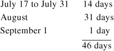
For Treasury coupon securities, a nonleap year is assumed to have 365 days. The number of days between settlement and the next coupon payment is therefore the actual number of days between the two dates. The day count convention for a coupon-bearing Treasury security is said to be “actual/actual,” which means the actual number of days in a month and the actual number of days in the coupon period. For example, consider a Treasury bond whose last coupon payment was on March 1; the next coupon would be six months later on September 1. Suppose that this bond is purchased with a settlement date of July 17. The actual number of days between July 17 (the settlement date) and September 1 (the date of the next coupon payment) is 46 days (the actual number of days in the coupon period is 184), as shown below:
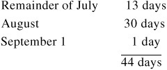
In contrast to the actual/actual day count convention for coupon-bearing Treasury securities, for corporate and municipal bonds and agency securities, the day count convention is “30/360.” That is, each month is assumed to have 30 days and each year 360 days. For example, suppose that the security in our previous example is not a coupon-bearing Treasury security but instead either a coupon-bearing corporate bond, municipal bond, or agency security. The number of days between July 17 and September 1 is shown below:
Compounding
Once the number of days between the settlement date and the next coupon date is determined, the present value formula must be modified because the cash-flows will not be received six months (one full period) from now. The Street convention is to compute the price is as follows:
1. Determine the number of days in the coupon period.
2. Compute the following ratio:
![]()
For a corporate bond, a municipal bond, and an agency security, the number of days in the coupon period will be 180 because a year is assumed to have 360 days. For a coupon-bearing Treasury security, the number of days is the actual number of days. The number of days in the coupon period is called the basis.
3. For a bond with n coupon payments remaining to maturity, the price is
![]()
p = price ($)
c = semiannual coupon payment ($)
M = maturity value
n = number of coupon payments remaining
i = periodic interest rate (required yield divided by 2) (in decimal)
The period (exponent) in the formula for determining the present value can be expressed generally as t −1 + w. For example, for the first cash-flow, the period is 1 −1 + w, or simply w. For the second cash-flow, it is 2 −1 w, or simply 1 + w. If the bond has 20 coupon payments remaining, the last period is 20 −1 + w, or simply 19 + w.
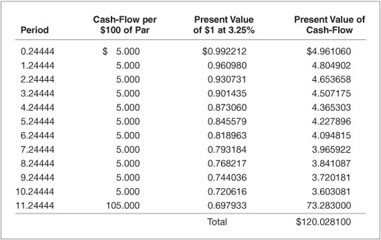
Illustration 4. Suppose that a corporate bond with a coupon rate of 10% maturing March 1, 2012 is purchased with a settlement date of July 17, 2006. What would the price of this bond be if it is priced to yield 6.5%?
The next coupon payment will be made on September 1, 2006. Because the bond is a corporate bond, based on a 30/360 day-count convention, there are 44 days between the settlement date and the next coupon date. The number of days in the coupon period is 180. Therefore,
![]()
The number of coupon payments remaining, n, is 12. The semiannual interest rate is 3.25% (6.5%/2).
The calculation based on the formula for the price is given in Exhibit 6–4. The price of this corporate bond would be $120.0281 per $100 par value. The price calculated in this way is called the full price or dirty price because it reflects the portion of the coupon interest that the buyer will receive but that the seller has earned.
EXHIBIT 6–4
Price Calculation When a Bond Is Purchased between Coupon Payments
Accrued Interest and the Clean Price
The buyer must compensate the seller for the portion of the next coupon interest payment the seller has earned but will not receive from the issuer because the issuer will send the next coupon payment to the buyer. This amount is called accrued interest and depends on the number of days from the last coupon payment to the settlement date.5 The accrued interest is computed as follows:
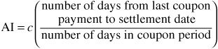
AI = accrued interest ($)
c = semiannual coupon payment ($)
Illustration 5. Let’s continue with the hypothetical corporate bond in Illustration 4. Because the number of days between settlement (July 17, 2006) and the next coupon payment (September 1, 2006) is 44 days and the number of days in the coupon period is 180, the number of days from the last coupon payment date (March 1, 2006) to the settlement date is 136 (180 – 44). The accrued interest per $100 of par value is
![]()
The full or dirty price includes the accrued interest that the seller is entitled to receive. For example, in the calculation of the full price in Exhibit 6–4, the next coupon payment of $5 is included as part of the cash-flow. The clean price or flat price is the full price of the bond minus the accrued interest.
The price that the buyer pays the seller is the full price. It is important to note that in calculation of the full price, the next coupon payment is a discounted value, but in calculation of accrued interest, it is an undiscounted value. Because of this market practice, if a bond is selling at par and the settlement date is not a coupon date, the yield will be slightly less than the coupon rate. Only when the settlement date and coupon date coincide is the yield equal to the coupon rate for a bond selling at par.
In the U.S. market, the convention is to quote a bond’s clean or flat price. The buyer, however, pays the seller the full price. In some non-U.S. markets, the full price is quoted.
CONVENTIONAL YIELD MEASURES
In the preceding section we explained how to compute the price of a bond given the required yield. In this section we’ll show how various yield measures for a bond are calculated given its price. First let’s look at the sources of potential return from holding a bond.
An investor who purchases a bond can expect to receive a dollar return from one or more of the following sources:
• The coupon interest payments made by the issuer
• Any capital gain (or capital loss—negative dollar return) when the bond matures, is called, or is sold
• Income from reinvestment of the coupon interest payments
This last source of dollar return is referred to as interest-on-interest.
Three yield measures are commonly cited by market participants to measure the potential return from investing in a bond—current yield, yield-to-maturity, and yield-to-call. These yield measures are expressed as a percent return rather than as a dollar return. However, any yield measure should consider each of the three potential sources of return just cited. Below we discuss these three yield measures and assess whether they consider the three sources of potential return.
Current Yield
The current yield relates the annual coupon interest to the market price. The formula for the current yield is
![]()
Illustration 6. The current yield for an 18-year, 6% coupon bond selling for $700.89 per $1,000 par value is 8.56%, as shown below:
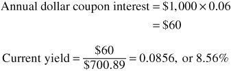
The current yield considers only the coupon interest and no other source of return that will affect an investor’s return. For example, in Illustration 6, no consideration is given to the capital gain that the investor will realize when the bond matures. No recognition is given to a capital loss that the investor will realize when a bond selling at a premium matures. In addition, interest-on-interest from reinvesting coupon payments is ignored.
Yield-to-Maturity
The yield or internal rate of return on any investment is the interest rate that will make the present value of the cash-flows equal to the price (or initial investment).6 The yield-to-maturity is computed in the same way as the yield; the cash-flows are those which the investor would realize by holding the bond to maturity. For a semiannual-pay bond, doubling the interest rate or discount rate gives the yield-to-maturity.
The calculation of a yield involves a trial-and-error procedure. Practitioners usually use calculators or software to obtain a bond’s yield-to-maturity. The following illustration shows how to compute the yield-to-maturity for a bond.
Illustration 7. In Illustration 6 we computed the current yield for an 18-year, 6% coupon bond selling for $700.89. The maturity value for this bond is $1,000. The yield-to-maturity for this bond is 9.5%, as shown in Exhibit 6–5. Cash-flows for the bond are
EXHIBIT 6–5
Computation of Yield-to-Maturity for an 18-Year, 6% Coupon Bond Selling at $700.89

• 36 coupon payments of $30 every six months
• $1,000 36 six-month periods from now
Different interest rates must be tried until one is found that makes the present value of the cash-flows equal to the price of $700.89. Because the coupon rate on the bond is 6% and the bond is selling at a discount, the yield must be greater than 6%. Exhibit 6–5 shows the present value of the cash-flows of the bond for semiannual interest rates from 3.25% to 4.75% (corresponding to annual interest rates from 6.5% to 9.50%). As can be seen, when a 4.75% interest rate is used, the present value of the cash-flows is $700.89. Therefore, the yield-to-maturity is 9.50% (4.75% × 2).
The yield-to-maturity considers the coupon income and any capital gain or loss that the investor will realize by holding the bond to maturity. The yield-to- maturity also considers the timing of the cash-flows. It does consider interest-on-interest; however, it assumes that the coupon payments can be reinvested at an interest rate equal to the yield-to-maturity. Thus, if the yield-to-maturity for a bond is 9.5%, to earn that yield, the coupon payments must be reinvested at an interest rate equal to 9.5%. The following example clearly demonstrates this.
Suppose that an investor has $700.89 and places the funds in a certificate of deposit (CD) that pays 4.75% every six months for 18 years, or 9.5% per year. At the end of 18 years, the $700.89 investment will grow to $3,726. Instead, suppose that the investor buys a 6%, 18-year bond selling for $700.89. This is the same as the price of our bond in Illustration 7. The yield-to-maturity for this bond is 9.5%. The investor would expect that at the end of 18 years, the total dollars from the investment will be $3,726.
Let’s look at what he will receive. There will be 36 semiannual interest payments of $30, which will total $1,080. When the bond matures, the investor will receive $1,000. Thus the total dollars that he will receive is $2,080 if he holds the bond to maturity, but this is $1,646 less than the $3,726 necessary to produce a yield of 9.5% (4.75% semiannually). How is this deficiency supposed to be made up? If the investor reinvests the coupon payments at a semiannual interest rate of 4.75% (or a 9.5% annual rate), it is a simple exercise to demonstrate that the interest earned on the coupon payments will be $1,646. Consequently, of the $3,025 total dollar return ($3,726 – $700.89) necessary to produce a yield of 9.5%, about 54% ($1,646 divided by $3,025) must be generated by reinvesting the coupon payments.
Clearly, the investor will realize the yield-to-maturity stated at the time of purchase only if (1) the coupon payments can be reinvested at the yield-to-maturity and (2) if the bond is held to maturity. With respect to the first assumption, the risk that an investor faces is that future reinvestment rates will be less than the yield-to-maturity at the time the bond is purchased. This risk is referred to as reinvestment risk. If the bond is not held to maturity, the price at which the bond may have to be sold is less than its purchase price, resulting in a return that is less than the yield-to-maturity. The risk that a bond will have to be sold at a loss because interest rates rise is referred to as interest-rate risk.
Reinvestment Risk
There are two characteristics of a bond that determine the degree of reinvestment risk. First, for a given yield-to-maturity and a given coupon rate, the longer the maturity, the more the bond’s total dollar return is dependent on the interest-on-interest to realize the yield-to-maturity at the time of purchase. That is, the greater the reinvestment risk. The implication is that the yield-to-maturity measure for long-term coupon bonds tells little about the potential yield that an investor may realize if the bond is held to maturity. In high-interest-rate environments, the interest-on-interest component for long-term bonds may be as high as 80% of the bond’s potential total dollar return.
The second characteristic that determines the degree of reinvestment risk is the coupon rate. For a given maturity and a given yield-to-maturity, the higher the coupon rate, the more dependent the bond’s total dollar return will be on the reinvestment of the coupon payments in order to produce the yield-to-maturity at the time of purchase. This means that holding maturity and yield-to-maturity constant, premium bonds will be more dependent on interest-on-interest than bonds selling at par. For zero-coupon bonds, none of the bond’s total dollar return is dependent on interest-on-interest; a zero-coupon bond carries no reinvestment risk if held to maturity.
Interest-Rate Risk
As we explained in the preceding section, a bond’s price moves in the direction opposite to the change in interest rates. As interest rates rise (fall), the price of a bond will fall (rise). For an investor who plans to hold a bond to maturity, the change in the bond’s price before maturity is of no concern; however, for an investor who may have to sell the bond prior to the maturity date, an increase in interest rates after the bond is purchased will mean the realization of a capital loss. Not all bonds have the same degree of interest-rate risk. In Chapter 7, the characteristics of a bond that determine its interest-rate risk are discussed.
Given the assumptions underlying yield-to-maturity, we can now demonstrate that yield-to-maturity has limited value in assessing the potential return of bonds. Suppose that an investor who has a five-year investment horizon is considering the following four option-free bonds:
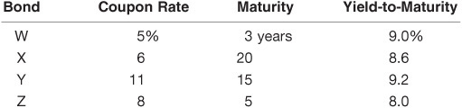
Assuming that all four bonds are of the same credit quality, which one is the most attractive to this investor? An investor who selects bond Y because it offers the highest yield-to-maturity is failing to recognize that the bond must be sold after five years, and the selling price of the bond will depend on the yield required in the market for 10-year, 11% coupon bonds at that time. Hence there could be a capital gain or capital loss that will make the return higher or lower than the yield-to-maturity promised now. Moreover, the higher coupon rate on bond Y relative to the other three bonds means that more of this bond’s return will be dependent on the reinvestment of coupon interest payments.
Bond W offers the second highest yield-to-maturity. On the surface, it seems to be particularly attractive because it eliminates the problem faced by purchasing bond Y of realizing a possible capital loss when the bond must be sold before the maturity date. In addition, the reinvestment risk seems to be less than for the other three bonds because the coupon rate is the lowest. However, the investor would not be eliminating the reinvestment risk because after three years she must reinvest the proceeds received at maturity for two more years. The return that the investor will realize will depend on interest rates three years from now, when the investor must roll over the proceeds received from the maturing bond.
Which is the best bond? The yield-to-maturity doesn’t seem to help us identify the best bond. The answer depends on the expectations of the investor. Specifically, it depends on the interest rate at which the coupon interest payments can be reinvested until the end of the investor’s investment horizon. Also, for bonds with a maturity longer than the investment horizon, it depends on the investor’s expectations about interest rates at the end of the investment horizon. Consequently, any of these bonds can be the best investment vehicle based on some reinvestment rate and some future interest rate at the end of the investment horizon. In the next section we present an alternative return measure for assessing the potential performance of a bond.
Yield-to-Maturity for a Zero-Coupon Bond
When there is only one cash-flow, it is much easier to compute the yield on an investment. A zero-coupon bond is characterized by a single cash-flow resulting from an investment. Consequently, the following formula can be applied to compute the yield-to-maturity for a zero-coupon bond:
y = (future value per dollar invested)1/n −1

Once again, doubling y gives the yield-to-maturity. Remember that the number of periods used in the formula is double the number of years.
Illustration 8. The yield-to-maturity for a zero-coupon bond selling for $274.78 with a maturity value of $1,000, maturing in 15 years, is 8.8%, as computed below:
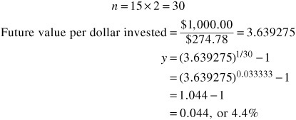
Doubling 4.4% gives the yield-to-maturity of 8.8%.
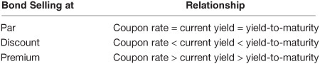
Relationship among Coupon Rate, Current Yield, and Yield-to-Maturity
The following relationship should be recognized between the coupon rate, current yield, and yield-to-maturity:
Problem with the Annualizing Procedure
Multiplying a semiannual interest rate by 2 will give an underestimate of the effective annual yield. The proper way to annualize the semiannual yield is by applying the following formula:
Effective annual yield = (1 + periodic interest rate)k −1
where
k = number of payments per year
For a semiannual-pay bond, the formula can be modified as follows:
Effective annual yield = (1 + semiannual interest rate)2 −1
Effective annual yield = (1 + y)2 −1
For example, in Illustration 7, the semiannual interest rate is 4.75%, and the effective annual yield is 9.73%, as shown below:
Effective annual yield=(1.0475)2 −1
=1.0973 −1
=0.0973, or 9.73%
Although the proper way for annualizing a semiannual interest rate is given in the preceding formula, the convention adopted in the bond market is to double the semiannual interest rate. The yield-to-maturity computed in this manner—doubling the semiannual yield—is called a bond-equivalent yield. In fact, this convention is carried over to yield calculations for other types of fixed income securities.
Yield-to-Call
For a callable bond, investors also compute another yield (or internal rate of return) measure, the yield-to-call. The cash-flows for computing the yield-to-call are those which would result if the issue were called on some assumed call date. Two commonly used call dates are the first call date and the first par call date. The yield-to-call is the interest rate that will make the present value of the cash-flows if the bond is held to the assumed call date equal to the price of the bond (i.e., the full price).
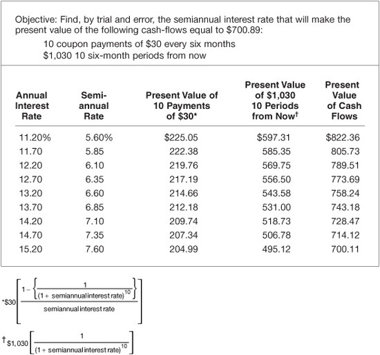
Illustration 9. In Illustrations 6 and 7, we computed the current yield and yield-to-maturity for an 18-year, 6% coupon bond selling for $700.89. Suppose that this bond is first callable in five years at $1,030. The cash-flows for this bond if it is called in five years are
• 10 coupon payments of $30 every six months
• $1,030 in 10 six-month periods from now
The interest rate we seek is one that will make the present value of the cash-flows equal to $700.89. From Exhibit 6–6, it can be seen that when the interest rate is 7.6%, the present value of the cash-flows is $700.11, which is close enough to $700.89 for our purposes. Therefore, the yield-to-call on a bond-equivalent basis is 15.2% (double the periodic interest rate of 7.6%).
EXHIBIT 6–6
Computation of Yield-to-Call for an 18-Year, 6% Coupon Bond Callable in 5 Years at $1,030, Selling at $700.89
According to the conventional approach, conservative investors will compute the yield-to-call and yield-to-maturity for a callable bond selling at a premium, selecting the lower of the two as a measure of potential return. It is the smaller of the two yield measures that investors would use to evaluate the yield for a bond. Some investors calculate not just the yield to the first call date and yield to first par call date but the yield to all possible call dates. Because most bonds can be called at any time after the first call date, the approach has been to compute the yield to every coupon anniversary date following the first call date. Then all calculated yields-to-call and the yield-to-maturity are compared. The lowest of these yields is called the yield-to-worst. The conventional approach would have us believe that this yield is the appropriate one a conservative investor should use.
Let’s take a closer look at the yield-to-call as a measure of the potential return of a callable bond. The yield-to-call does consider all three sources of potential return from owning a bond. However, as in the case of the yield-to-maturity, it assumes that all cash-flows can be reinvested at the computed yield—in this case, the yield-to-call—until the assumed call date. As we noted earlier in this chapter, this assumption may be inappropriate. Moreover, the yield-to-call assumes that (1) the investor will hold the bond to the assumed call date and (2) the issuer will call the bond on that date.
The assumptions underlying the yield-to-call are often unrealistic. They do not take into account how an investor will reinvest the proceeds if the issue is called. For example, consider two bonds, M and N. Suppose that the yield-to-maturity for bond M, a five-year option-free bond, is 10%, whereas for bond N the yield-to-call, assuming that the bond will be called in three years, is 10.5%. Which bond is better for an investor with a five-year investment horizon? It’s not possible to tell from the yields cited. If the investor intends to hold the bond for five years and the issuer calls the bond after three years, the total dollars that will be available at the end of five years will depend on the interest rate that can be earned from reinvesting funds from the call date to the end of the investment horizon.
More will be said about the analysis of callable bonds in Chapter 40.
Yield (Internal Rate of Return) for a Portfolio
The yield for a portfolio of bonds is not simply the average or weighted average of the yield-to-maturity of the individual bond issues. It is computed by determining the cash-flows for the portfolio and then finding the interest rate that will make the present value of the cash-flows equal to the market value of the portfolio.7 As with any yield measure, it suffers from the same assumptions.
Illustration 10. Consider the following three-bond portfolio:8

The portfolio’s total market value is $57,259,000. The cash-flow for each bond in the portfolio and for the whole portfolio is as follows:
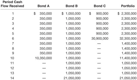
To determine the yield (internal rate of return) for this three-bond portfolio, the interest rate that makes the present value of the cash-flows shown in the last column of the table above equal to $57,259,000 (the total market value of the portfolio) must be found. If an interest rate of 4.77% is used, the present value of the cash-flows will equal $57,259,000. Doubling 4.77% gives 9.54%, which is the yield on the portfolio on a bond-equivalent basis.
Yield Measure for Floating-Rate Securities
The coupon rate for a floating-rate security changes periodically based on some reference rate (such as LIBOR).9 Because the value for the reference rate in the future is not known, it is not possible to determine the cash-flows. This means that a yield-to-maturity cannot be calculated.
A conventional measure used to estimate the potential return for a floating-rate security is the security’s discount margin. This measure estimates the average spread or margin over the reference rate that the investor can expect to earn over the life of the security. The procedure for calculating the discount margin is as follows:
1. Determine the cash-flows assuming that the reference rate does not change over the life of the security.
2. Select a margin (spread).
3. Discount the cash-flows found in step 1 by the current value of the reference rate plus the margin selected in step 2.
4. Compare the present value of the cash-flows as calculated in step 3 to the price. If the present value is equal to the security’s price, the discount margin is the margin assumed in step 2. If the present value is not equal to the security’s price, go back to step 2 and try a different margin.
For a security selling at par, the discount margin is simply the spread over the reference rate.
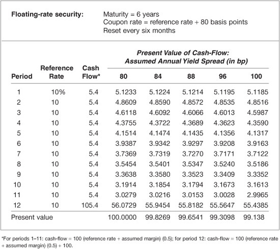
Illustration 11. To illustrate the calculation, suppose that a six-year floating-rate security selling for 99.3098 pays a rate based on some reference rate index plus 80 basis points. The coupon rate is reset every six months. Assume that the current value for the reference rate is 10%. Exhibit 6–7 shows the calculation of the discount margin for this security. The second column shows the current discounted value for the reference rate (10%). The third column sets forth the cash-flows for the security. The cash-flow for the first 11 periods is equal to one-half the current value for the reference rate (5%) plus the semiannual spread of 40 basis points multiplied by 100. In the twelfth six-month period, the cash-flow is 5.4 plus the maturity value of 100. The top row of the last five columns shows the assumed margin. The rows below the assumed margin show the present value of each cash-flow. The last row gives the total present value of the cash-flows. For the five assumed yield spreads, the present value is equal to the price of the floating-rate security (99.3098) when the assumed margin is 96 basis points. Therefore, the discount margin on a semiannual basis is 48 basis points and 96 basis points on an annual basis. (Notice that the discount margin is 80 basis points, the same as the spread over the reference rate, when the security is selling at par.)
EXHIBIT 6–7
Calculation of the Discount Margin for a Floating-Rate Security
There are two drawbacks of the discount margin as a measure of the potential return from investing in a floating-rate security. First, this measure assumes that the reference rate will not change over the life of the security. Second, if the floating-rate security has a cap or floor, this is not taken into consideration. Techniques described in Chapter 40 can allow interest rate volatility to be considered and can handle caps or floors.
TOTAL RETURN ANALYSIS
If conventional yield measures such as the yield-to-maturity and yield-to-call offer little insight into the potential return of a bond, what measure of return can be used? The proper measure is one that considers all three sources of potential dollar return over the investment horizon. This requires that an investor first project the total future dollars over an investment horizon. The return is then the interest rate that will make the bond’s price (full price) grow to the projected total future dollars at the end of the investment horizon. The yield computed in this way is known as the total return, also referred to as the horizon return. In this section we explain this measure and demonstrate how it can be applied in assessing the potential return from investing in a bond.
Calculating the Total Return
The total return requires that the investor specify
• An investment horizon
• A reinvestment rate
• A selling price for the bond at the end of the investment horizon (which depends on the assumed yield at which the bond will sell at the end of the investment horizon)
More formally, the steps for computing a total return over some investment horizon are as follows.
Step 1: Compute the total coupon payments plus the interest-on-interest based on an assumed reinvestment rate. The reinvestment rate is one-half the annual interest rate that the investor believes can be earned on the reinvestment of coupon interest payments.
The total coupon payments plus interest-on-interest can be calculated using the formula for the future value of an annuity (see the Appendix to this book) as shown:
Coupon plus interest-on-interest
= semiannual coupon 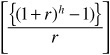
h = length of the investment horizon (in semiannual periods)
r = assumed semiannual reinvestment rate
Step 2: Determine the projected sale price at the end of the investment horizon. The projected sale price will depend on the projected yield on comparable bonds at the end of the investment horizon.
Step 3: Add the values computed in steps 1 and 2. The sum is the total future dollars that will be received from the investment given the assumed reinvestment rate and projected required yield at the end of the investment horizon.
Step 4: To obtain the semiannual total return, use the following formula:
![]()
Step 5: Because coupon interest is assumed to be paid semiannually, double the interest rate found in step 4. The resulting interest rate is the total return expressed on a bond-equivalent basis. Alternatively, the total return can be expressed on an effective annual interest rate basis by using the following formula:
(1 + semiannual total return)2 −1
Illustration 12. Suppose that an investor with a three-year investment horizon is considering purchasing a 20-year, 8% coupon bond for $828.40. The yield-to-maturity for this bond is 10%. The investor expects that he can reinvest the coupon interest payments at an annual interest rate of 6% and that at the end of the investment horizon the 17-year bond will be selling to offer a yield-to-maturity of 7%. The total return for this bond is computed in Exhibit 6–8.
EXHIBIT 6–8
Illustration of Total Return Calculation
Assumptions:
Bond = 8% 20-year bond selling for $828.40 (yield-to-maturity is 10%)
Annual reinvestment rate = 6%
Investment horizon = 3 years
Yield for 17-year bonds at end of investment horizon = 7%
Step 1: Compute the total coupon payments plus the interest-on-interest assuming an annual reinvestment rate of 6%, or 3% every six months. The coupon payments are $40 every six months for three years or six periods (the investment horizon). The total coupon interest plus interest-on-interest is
![]()
Step 2: The projected sale price at the end of 3 years, assuming that the required yield-to-maturity for 17-year bonds is 7%, is found by determining the present value of 34 coupon payments of $40 plus the present value of the maturity value of $1,000, discounted at 3.5%. The price can be shown to be $1,098.51.
Step 3: Adding the amount in steps 1 and 2 gives total future dollars of $1,357.25.
Step 4: Compute the following:
Step 5: Doubling 8.58% gives a total return of 17.16% on a bond-equivalent basis. On an effective annual interest-rate basis, the total return is

Objections to the total return analysis cited by some portfolio managers are that it requires them to make assumptions about reinvestment rates and future yields and forces a portfolio manager to think in terms of an investment horizon. Unfortunately, some portfolio managers find comfort in meaningless measures such as the yield-to-maturity because it is not necessary to incorporate any expectations. As explained below, the total return framework enables the portfolio manager to analyze the performance of a bond based on different interest-rate scenarios for reinvestment rates and future market yields. By investigating multiple scenarios, the portfolio manager can see how sensitive the bond’s performance is to each scenario. There is no need to assume that the reinvestment rate will be constant for the entire investment horizon.
For portfolio managers who want to use the market’s expectations of short-term reinvestment rates and the yield on the bond at the end of the investment horizon, implied forward rates can be calculated from the yield-curve. Implied forward rates are explained in Chapters 8 and 36, and are calculated based on arbitrage arguments. A total return computed using implied forward rates is called an arbitrage-free total return.
Scenario Analysis
Because the total return depends on the reinvestment rate and the yield at the end of the investment horizon, portfolio managers assess performance over a wide range of scenarios for these two variables. This approach is referred to as scenario analysis.
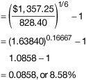
Illustration 13. Suppose that a portfolio manager is considering the purchase of bond A, a 20-year, 9% option-free bond selling at $109.896 per $100 of par value. The yield-to-maturity for this bond is 8%. Assume also that the portfolio manager’s investment horizon is three years and that the portfolio manager believes that the reinvestment rate can vary from 3% to 6.5% and that the yield at the end of the investment horizon can vary from 5% to 12%.
The top panel of Exhibit 6–9 shows the total future dollars at the end of three years under various scenarios. The bottom panel shows the total return (based on the effective annualizing of the six-month total return). The portfolio manager knows that the maximum and minimum total return for the scenarios analyzed will be 16.72% and –1.05%, respectively, and the scenarios under which each will be realized. If the portfolio manager faces three-year liabilities guaranteeing, say, 6%, the major consideration is scenarios that will produce a three-year total return of less than 6%. These scenarios can be determined from Exhibit 6–9.
EXHIBIT 6–9
Scenario Analysis for Bond A

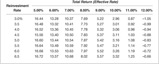
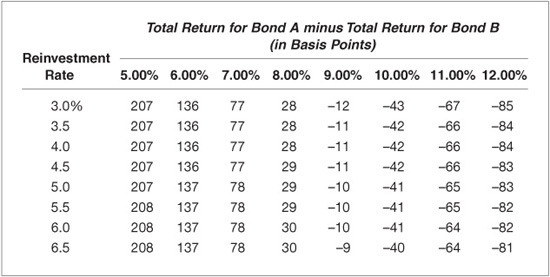
Illustration 14. Suppose that the same portfolio manager owns bond B, a 14-year option-free bond with a coupon rate of 7.25% and a current price of $94.553 per $100 par value. The yield-to-maturity is 7.9%. Exhibit 6–10 reports the total future dollars and total return over a three-year investment horizon under the same scenarios as Exhibit 6–9. A portfolio manager considering swapping from bond B to bond A would compare the relative performance of the two bonds as reported in Exhibits 6–9 and 6–10. Exhibit 6–11 shows the difference between the performance of the two bonds in basis points. This comparative analysis assumes that the two bonds are of the same investment quality and ignores the financial accounting and tax consequences associated with the disposal of bond B to acquire bond A.
EXHIBIT 6–10
Scenario Analysis for Bond B
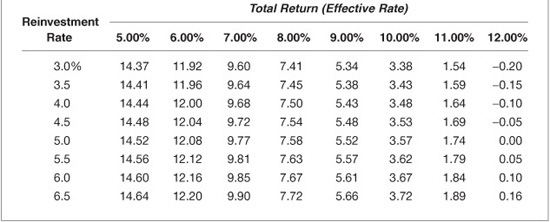
EXHIBIT 6–11
Scenario Analysis Showing the Relative Performance of Bonds A and B
Evaluating Potential Bond Swaps
Portfolio managers commonly swap an existing bond in a portfolio for another bond. Bond swaps can be categorized as pure yield pickup swaps, substitution swaps, intermarket-spread swaps, or rate-anticipation swaps. Total return analysis can be used to assess the potential return from a swap.
• Pure yield pickup swap. Switching from one bond to another that has a higher yield is called a pure yield pickup swap. The swap may be undertaken to achieve either higher current coupon income or higher yield-to-maturity or both. No expectation is made about changes in interest rates, yield spreads, or credit quality.
• Rate-anticipation swap. A portfolio manager who has expectations about the future direction of interest rates will use bond swaps to position the portfolio to take advantage of the anticipated interest-rate move. These are known as rate-anticipation swaps. If rates are expected to fall, for example, bonds with a greater price volatility will be swapped for existing bonds in the portfolio with lower price volatility (to take advantage of the larger change in price that will result if interest rates do in fact decline). The opposite will be done if rates are expected to rise.
• Intermarket-spread swap. These swaps are undertaken when the portfolio manager believes that the current yield spread between two bonds in the market is out of line with its historical yield spread and that the yield spread will realign by the end of the investment horizon. Yield spreads between bonds exist for the following reasons: (1) there is a difference in the credit quality of bonds (e.g., between Treasury bonds and double-A-rated public utility bonds of the same maturity), or (2) there are differences in the features of corporate bonds that make them more or less attractive to investors (for example, callable and noncallable bonds, and putable and nonputable bonds).
• Substitution swap. In a substitution swap, a portfolio manager swaps one bond for another bond that is thought to be identical in terms of coupon, maturity, price sensitivity to interest-rate changes, and credit quality, but that offers a higher yield. This swap depends on a capital market imperfection. Such situations sometimes exist in the bond market because of temporary market imbalances. The risk that the portfolio manager faces is that the bond purchased may not be identical to the bond for which it is exchanged. For example, if credit quality is not the same, the bond purchased may be offering a higher yield because of higher credit risk rather than because of a market imbalance.
Comparing Municipal and Corporate Bonds
The conventional methodology for comparing the relative performance of a tax-exempt municipal bond and a taxable corporate bond is to compute the taxable equivalent yield. The taxable equivalent yield is the yield that must be earned on a taxable bond in order to produce the same yield as a tax-exempt municipal bond. The formula is
![]()
For example, suppose that an investor in the 35% marginal tax bracket is considering a 10-year municipal bond with a yield-to-maturity of 4.5%. The taxable equivalent yield is
![]()
If the yield-to-maturity offered on a comparable-quality corporate bond with 10 years to maturity is more than 6.92%, those who use this approach would recommend that the corporate bond be purchased. If, instead, a yield-to-maturity of less than 6.92% on a comparable corporate bond is offered, the investor should invest in the municipal bond.
What’s wrong with this approach? The tax-exempt yield of the municipal bond and the taxable equivalent yield suffer from the same limitations we discussed with respect to yield-to-maturity. Consider the difference in reinvestment opportunities for a corporate and a municipal bond. For the former, coupon payments will be taxed; therefore, the amount to be reinvested is not the entire coupon payment but an amount net of taxes. In contrast, because the coupon payments are free from taxes for a municipal bond, the entire coupon can be reinvested.
The total return framework can accommodate this situation by allowing us to explicitly incorporate the reinvestment opportunities. There is another advantage to the total return framework as compared with the conventional taxable equivalent yield approach. Changes in tax rates (because the investor expects either her tax rate to change or the tax structure to change) can be incorporated into the total return framework.
KEY POINTS
• The price of a bond is equal to the present value of the expected cash flow.
• For bonds with embedded options, the cash-flow is difficult to estimate.
• The required yield used to discount the cash-flow is determined by the yield offered on comparable securities.
• The two most popular yield measures cited in the bond market are the yield-to-maturity and yield-to-call. Both yield measures consider the coupon interest and any capital gain (or loss) at the maturity date or call date in the case of the yield-to-call.
• The coupon interest and capital gain (or loss), however, are only two of the three components of the potential dollar return from owning a bond until it matures or is called. The other component is the reinvestment of coupon income, commonly referred to as the interest-on-interest component. This component can be as large as 80% of a bond’s total dollar return.
• The yield-to-maturity assumes that the coupon payments can be reinvested at the calculated yield-to-maturity.
• The yield-to-call assumes that the coupon payments can be reinvested at the calculated yield-to-call.
• A better measure of the potential return from holding a bond over a predetermined investment horizon is the total return measure. This measure considers all three sources of potential dollar return and can be used to analyze bond swaps and bond performance.