CHAPTER
FIFTY-FIVE
MANAGING THE SPREAD RISK OF CREDIT PORTFOLIOS USING THE DURATION TIMES SPREAD MEASURE

ARIK BEN DOR, PH.D.

Director, Barclays Capital

LEV DYNKIN, PH.D.

Managing Director, Barclays Capital

JAY HYMAN, PH.D.

Managing Director, Barclays Capital

The standard presentation of the asset allocation in a portfolio or a benchmark is in terms of percentage of market value. It is widely recognized that this is not sufficient for fixed income portfolios, where differences in duration can cause two portfolios with the same allocation of market weights to have extremely different exposures to macro-level risks. As a result, fixed income portfolio managers have become accustomed to expressing their allocations in terms of contributions to duration—the product of the percentage of portfolio market value represented by a given market cell and the average duration of securities comprising that cell. This represents the sensitivity of the portfolio to a parallel shift in yields across all securities within this market cell. For credit portfolios, the corresponding measure would be contributions to spread duration, measuring the sensitivity to a parallel shift in spreads. Determining the set of active spread duration bets (the differences between the exposures of the portfolio and the benchmark) from various market cells and/or issuers is one of the primary decisions taken by credit portfolio managers.

Yet all spread durations were not created equal. Just as one could create a portfolio that matches the benchmark exactly by market weights, but clearly takes more credit risk (e.g., by investing in the longest duration credits within each cell), one could match the benchmark exactly by spread duration contributions and still take more credit risk—by choosing the credits with the widest spreads within each cell. These credits presumably trade wider than their peer groups for a reason; that is, the market consensus has determined that they are more risky—and are often referred to as “high-beta” credits, because their spreads tend to react more strongly than the rest of the market to any systematic shock.

Based on this idea, and following an extensive analysis of corporate bonds’ spread behavior, we have advocated since 2005 a new measure of risk sensitivity that utilizes spreads as a fundamental part of the credit portfolio management process. To reflect the view that higher spread credits represent greater exposures to sector-specific risks, we represent sector exposures by contributions to duration times spread (DTS), computed as the product of market weight, spread duration, and spread. The shift from spread duration exposures to DTS exposures as the measure of market risk embraces a different paradigm for credit-spread movement—in the form of relative spread changes rather than parallel shifts in spread.

The paradigm shift resulting from the DTS concept has many implications for portfolio managers, both in terms of the way they manage exposures to industry and quality factors (systematic risk) and in terms of their approach to issuer exposures (non-systematic risk). First, modeling spread changes in relative rather than absolute terms generates improved forward-looking estimates of excess return volatility. Second, for computing the hedge ratios needed to form market-neutral credit trades, DTS is superior to “empirical betas” as a measure of market sensitivity. Third, for index replication, matching sector-quality allocations of a credit index in terms of contributions to DTS leads to improved tracking compared with matching the contributions to spread duration. This same way of viewing macro exposures can help to more accurately express active portfolio weights as well. Fourth, DTS-based issuer limits can be considered as an alternative to more standard caps on issuer market weight when imposing portfolio diversification constraints. Finally, the incorporation of the DTS approach into the design of multifactor risk models can help make such models more robust, more compact, and more accurate. In this chapter, we will explore each of these applications in turn, after a brief overview of the large body of evidence supporting the DTS concept.

THE NEED FOR A NEW MEASURE OF CREDIT SPREAD EXPOSURE

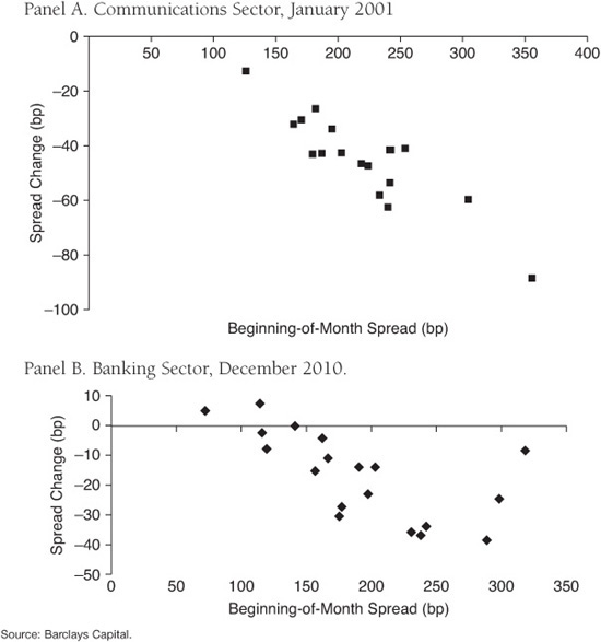
Two examples of market conditions when spread duration contributions do not suffice are shown in Exhibit 55–1. During the dot.com crisis, a relief rally in January 2001 led to a temporary tightening of spreads throughout the communications sector. However, that rally was not characterized by a purely parallel shift; rather, issuers with wider spreads tightened by more. Panel A displays the changes in spreads experienced in that month by the key issuers that made up the communications sector of the Barclays Capital Corporate Index.¹ Panel B shows the spread tightening in the key issuers in the banking sector during the month of December 2010; a similar effect is seen in this industry-wide rally.

EXHIBIT 55–1
Spread Changes of Key Issuers in the Communications and Banking Sectors of the Barclays Capital U.S. Corporate Index

Motivated by market events of this type, we conducted an extensive analysis of corporate bonds’ spread behavior and developed a new measure of spread risk sensitivity. As higher spread credits have greater exposures to sector-specific risks, we represent sector exposures by contributions to duration times spread (DTS), computed as the product of market weight, spread duration, and spread. An overweight of 5% to a market cell implemented by purchasing bonds with a spread of 80 bp and spread duration of three years will be considered to be equivalent to an overweight of 3% using bonds with an average spread of 50 bp and spread duration of eight years (0.05 × 0.80 × 3 = 0.03 × 0.50 × 8 = 0.12).

How does this make sense? As mentioned, a portfolio’s contribution to spread duration within a given market cell is its sensitivity to a parallel shift in spreads across all bonds in that cell. What is the intuition behind this new measure?

In fact, the intuition is very simple. Let us look at a simple expression for the return of a given bond due strictly to change in spread R_spread. Let D denote the spread duration of the bond and s its spread; the spread change return is then given by

It is quite easy to see that this equation is equivalent to

That is, just as spread duration is the sensitivity to an absolute change in spread (e.g., spreads widen by 5 bp), DTS is the sensitivity to a relative change in spread (e.g., spreads increase by 5% of their current levels). Note that this notion of relative spread change provides for a formal expression of the rough idea discussed above—that credits with wider spreads are riskier since they tend to experience greater spread changes in absolute terms.

Based on the absolute spread change approach in Eq. (55–1), the volatility of excess returns can be approximated by

while in the relative spread change approach of Eq. (55–2), excess return volatility follows

Given that the two representations above are equivalent, why should one of them be preferable to another? The key advantage of the DTS approach of Eq. (55–4) is that relative spread volatilities are much more stable than absolute spread volatilities. We found extensive empirical evidence that the volatility of absolute spread changes of U.S. corporate bonds (both systematic and idiosyncratic) is linearly proportional to spread level, irrespective of sector, maturity, credit quality or time period.² This implies that the second approach, based on relative spread changes, should generate more accurate projections of spread volatility.

SPREAD VOLATILITY AND DTS

The relation between the volatility of systematic spread changes and the average beginning-of-month spread level is plotted in Exhibit 55–2. The analysis was carried out using a large sample with more than 560,000 monthly observations on all constituents of the Barclays Capital Corporate and High-Yield Indices rated B or higher between September 1989 and January 2005.³ Bonds in each of the three main sectors (financials, industrials, and utilities) were divided into three equally populated duration buckets (short, medium, and long). Bonds in each duration bucket were then partitioned into prespecified cells based on spread. Spread cell breakpoints varied across sector and duration to ensure that each spread cell was well populated monthly.⁴ This procedure resulted in 66 distinct time series data sets; each consisted of a fairly homogeneous set of bonds with monthly data for their spreads and spread changes. The systematic spread change in a given cell each month was represented simply as the average spread change across all bonds that comprised that cell. We then calculated the time series volatility of these systematic spread changes and the average spread over time for each cell.

EXHIBIT 55–2
Time Series Volatility of Systematic Spread Changes vs. Spread Level

The results indicate an almost perfect linear relationship between spread volatility and the level of spread that can formally be expressed as:

Estimating a simple regression based on Eq. (55–5) provides an excellent fit to the data (R² in excess of 90%) with the slope coefficient θ equal to 9.1% using all observations and 9.4% if the three circled outliers are excluded.⁵ Furthermore, for a given level of spread, the differences across sectors and maturity buckets are fairly small. Hence, the historical volatility of systematic spread movements can be expressed quite compactly, with only minor dependence on sector or maturity, in terms of a relative spread change volatility of about 9% to 10% per month. That is, spread volatility for a market segment trading at 50 bp should be about 4.5–5.0 bp/month, whereas that of a market segment at 200 bp should be about 18–20 bp/month.

We also studied whether idiosyncratic spread volatility is similarly related to the level of spreads. We computed the standard deviation of the differences between all individual bonds’ spread changes and the average spread change of their respective cell, pooled across all bonds and months. This pooled measure of idiosyncratic spread volatility per market cell was then plotted against the median spread of the cell. We again found a very strong linear relationship between spread and idiosyncratic spread volatility, with a slope similar to that estimated for systematic volatility.

To corroborate these findings, we also investigated the relation between excess return volatility and DTS. If the volatility of systematic spread changes is proportional to the level of spread, then Eq. (55–4) implies that a portfolio’s excess return volatility should increase linearly with its DTS, with the slope equal to the volatility of relative spread changes. In addition, excess return volatility for portfolios with similar DTS should be approximately equal even if their spreads or spread durations differ.

To examine these predictions, bonds were assigned into DTS quintiles, which in turn were further subdivided into six equally populated buckets based on spread. The average excess returns and median DTS were calculated monthly for each bucket separately. These statistics were then used to compute the excess return volatility and average DTS for all time-series.

The results of this analysis are presented in Exhibit 55–3, which plots the time series volatility of excess returns for each of the quintile-bucket combinations against its average DTS. First, it is clear that excess return volatility increases with the level of DTS and that a straight line through the origin provides an excellent fit. This is indeed confirmed by a regression of the excess return volatility against the average DTS, which finds a fit of 98% and an insignificant intercept. Furthermore, the estimate of the slope coefficient (8.8%) is in line with the volatility of relative spread changes found in Exhibit 55–2 as expected. Second, observations representing the same DTS quintile exhibit very similar excess return volatilities despite large difference in their spreads and durations.⁶

EXHIBIT 55–3
Excess Return Volatility VS. DTS

In 2009, we re-examined whether the key findings underlying the DTS concept remained valid through the credit crisis of 2007–2009.⁷ We showed that the fundamental relationship between the level of spread and subsequent volatility persisted in a linear fashion across all sectors and credit ratings, although the proportionality factor increased from 10% to about 15%. While this implies that a long-term calibrated DTS model would not have fully captured spread risk during the crisis months, we demonstrated that it was far more effective than any other spread duration–based measure. The explicit use of spread in the DTS framework as a barometer of risk proved to be of paramount importance in managing credit portfolios during that volatile period.

The concept of spread proportionality and DTS are not limited only to U.S. corporate bonds. From a theoretical standpoint, we showed that structural credit risk models such as the Merton model imply a near-linear relationship between spread level and volatility.⁸ Subsequent empirical studies indeed found that the applicability of DTS extends to other spread asset classes with a significant default risk. For example, we investigated the dynamics of CDS spreads⁹ in both the U.S. dollar and euro markets using a different estimation approach, sample period and data frequency than those used in the original study of U.S. corporate bonds. Despite these differences in data and technique, we found clear evidence of a linear relation between spread volatility and spread level with a very similar slope.¹⁰ Similar results were documented for European corporate and sovereign bonds and emerging market sovereign debt denominated in U.S. dollars.¹¹

RISK PROJECTION: PREDICTING SPREAD VOLATILITY

Perhaps the most important requirement for managing a credit portfolio successfully is the ability to measure its risk accurately. A key benefit of DTS in the context of generating volatility forecasts is its use of current spread levels to quickly adapt to changing market conditions. In contrast, estimates based on past realized spread volatility can take longer to adapt, depending on the time window used for calibration. The selected time period is inherently subjective, and may not perfectly reflect the current state of the market.

The credit crisis of 2007–2009 provides an excellent opportunity to examine the differences between forecasts based on DTS and traditional measures relying on historical realized spread changes for at least two reasons. First, the magnitude of the crisis was unprecedented. Spreads of U.S. investment-grade bonds widened to an all-time high of more than 6%, from lows of around 1% in the benign 2003–2006 period. Similarly, spreads of high-yield bonds rose to more than 18% and credit default index swap (CDX) spreads increased by a factor of five. Not only the magnitude, but also the extraordinary speed at which spreads widened, caught many investors off guard, with risk estimates calibrated to the sustained “volatility drought” of the previous few years severely underestimating the spread risk of corporate bonds. Second, since the concept of DTS was first introduced in 2005, the crisis period presented a true out-of-sample test of its effectiveness.

Exhibit 55–4 shows the monthly spread changes of the Barclays Capital U.S. Corporate Index normalized by several projections of spread volatility from January 2006, well before the first signs of the crisis were observed, through March 2010, when markets were already in recovery mode. The first forecast of volatility, based on DTS, is the product of the spread level at the beginning of the month and the (approximate) relative spread volatility (10%/month) estimated in our original study, based on the analysis shown in Exhibit 55–2. The plot also includes two estimates using the realized volatility over a trailing 36-month window or during the entire history (since September 1989) available as of the start of each month.

EXHIBIT 55–4
Comparison of Volatility Forecasts Based on DTS and Historical Absolute Spread Changes

The exhibit illustrates that the forecast based on the trailing 36 months would have fit the low volatility level during the pre-crisis period quite well, but was susceptible to large sudden shocks such as in July 2007 and November 2007, which resulted in 5.1 and 6.3 standard deviation realizations, respectively. Although the estimator gradually adjusted to the change in market conditions, it continued to understate the level of risk more than a year after the crisis began, with an 8.4 standard deviation realization in September 2008.

In contrast, the “long-term” forecast was better prepared at the beginning of the crisis since it incorporated information from previous extreme market events such as the 1998 and 2002 crisis periods. While its forecast of volatility for July 2007, for example, was higher than that of the “short-term” estimator, it generated grossly underestimated risk projections toward the end of 2008. Because adjustment to changing market conditions is slow, the spread change in September 2008 would have corresponded to an 11.6 standard deviation event, using the forecast generated by the long-term volatility measure. Similarly, the estimator underestimated the magnitude of the spread tightening beginning in early 2009 as market conditions started to improve.

The DTS volatility estimates over the period were consistently superior to both forecasts using realized volatilities. The DTS-based forecasts quickly (albeit not perfectly) reflected both the increased level of risk since the crisis erupted and the reversal in market conditions in 2009, with most spread change realizations corresponding to less than two standard deviations. A notable exception was September 2008. Despite the already heightened level of spreads, the combined effect of Lehman Brothers’ and Washington Mutual’s defaults and the bailout of AIG in that month resulted in a 4.5 standard deviation event. However, as discussed, the forecasts using realized absolute spread volatility underestimated the risk by a factor of between two and three times more than the DTS-based forecast.

The credit crisis that began in 2007 affected not only corporate but also sovereign issuers. The deteriorating economic conditions in several of the euro area economies with high deficits and/or debt ratios subsequently raised solvency concerns among many investors. As a result, spreads of countries such as Portugal, Ireland, Italy, Greece, and Spain widened significantly in 2010 relative to German treasuries, to the point where the risk contribution of sovereign spreads in investment-grade bond indices grew larger than that of corporate bonds.¹² Many market participants had to suddenly re-evaluate their risk management practices. It was apparent that past volatilities of absolute spread changes could no longer serve as a basis for forward-looking risk projections in this market, as sovereign spreads had mostly been very tight and stable since the inception of the Euro in 1999. The DTS paradigm, keying on rising spread levels, does not require a long period of increased spread volatility to warrant an increase in forward-looking risk estimates. Furthermore, as mentioned earlier, theory suggests that DTS should apply to all securities with a credit component irrespective of the issuing entity, and earlier results indeed confirmed it is applicable to emerging market countries. Therefore, it is interesting to see to what extent using the DTS paradigm to project the spread risk of Euro sovereign issuers could have helped investors in this asset class.

Exhibit 55–5 compares the daily spread volatility of several Euro countries over two distinct periods, which roughly span the time period of the crisis. Volatility between August 2008 and July 2009 is represented on the horizontal axis, whereas the vertical axis reflects the volatility in the period from August 2009 to July 2010. The time partition was selected such that both periods have about the same length but correspond to different stages of the sovereign debt crisis. Each observation represents either the absolute or relative spread volatility of a particular country. Observations along the diagonal line indicate that the volatilities are the same over the two time periods.

EXHIBIT 55–5
Absolute and Relative Volatility of Daily Spread Changes for Selected European Sovereign Issuers

Two clear patterns can be observed in the plot. First, most of the observations representing absolute spread volatilities are located quite far above the line, pointing to a marked increase in volatility in the second period of the sample. In contrast, relative spread volatilities are quite stable, with almost all observations located near the straight line crossing the origin, which represents equal volatilities (absolute or proportional) in both periods. This is because the pick-up in volatility in the second period was accompanied by a similar increase in spreads. In particular, the daily volatility of absolute spread changes for Greece increased by a factor of almost 10 (from 5.9 to 51.6 bp), whereas in relative terms it only increased from 4.3% to 6.8%.

Second, the daily volatilities¹³ of relative spread changes in various countries are quite tightly clustered, ranging from 4.5% to a bit over 8%, whereas the range of absolute volatilities is much wider, ranging from 1.6 to more than 17 bp for Portugal and even higher for Greece. Furthermore, spread proportionality seems to capture well not only the spread dynamics of the countries that were in the center of the crisis (Portugal, Greece, Spain, Ireland, and Italy), but also countries that were less affected such as Belgium and France. While the exhibit suggests that absolute spread volatility also remained essentially unchanged for these two countries, using relative spreads offers the advantage of similar volatilities across all sovereign issuers.

Exhibits 55–4 and 55–5 provide an illustration of the advantage of the DTS approach compared with the risk estimated based on absolute spread changes. The DTS approach does not require a subjective selection of an historical calibration period, and allows for a rapid incorporation of market conditions as reflected in the level of spreads. This feature can be especially valuable in situations where market volatilities exceed any historical precedent, as illustrated in these two exhibits for the credit and sovereign crises of 2007–2010. It is also important to note that DTS-based risk forecasts can immediately adapt to changing conditions. Whereas models based on realized monthly volatility will only be updated at the end of a month, DTS estimates can be updated as soon as spread changes are marked—intra-month or even intra-day.

HEDGING: PREDICTING SENSITIVITIES TO MARKET SPREAD CHANGES

Another natural application of DTS is hedging. Consider an investor whose basic goal is to express a view favoring one issuer over another while taking as little directional market risk as possible. The primary driver of the performance of such a strategy should be the investor’s skill at forming views on issuers, while any systematic risk is to be minimized. The success or failure in isolating issuer-specific risk lies in his ability to forecast the market beta of each security over the return horizon.

Say we are considering a trade as of December 31, and plan to hold it in position for three months. The betas we would like to use for this hedge are the as-yet unknown ones that we will find ex post as we later review the returns realized from January through March. What is the best forecast we can make given the data we have at our disposal? An obvious approach would be to use DTS. Since the DTS contribution of a position measures its systematic spread exposure, DTS neutrality should be the best way to hedge the market exposure of an issuer-specific trade that goes long one issuer and short another.

To examine this question, we conducted a study that compared two different methods for forecasting the market betas of individual CDS over a given period using only data available at the beginning of the period.¹⁴ The first relied on the ratio of the DTS (in this case, risky PV01 times spread) of the individual CDS to that of the market as of the beginning of the period. The second approach was one commonly used by investors, based on the empirical beta of the individual CDS to the market from the prior period. We divided the dataset, which contained roughly three years of weekly data, into nonoverlapping periods of equal length, either 26 weeks or 52 weeks each. For each period but the first, the beta of each security was estimated using the two methods: either by using the spread as of the start of the period, or by using the security’s beta from the prior period. We then regressed the realized beta during the period on each of these two candidate predictors. Since there were 84 issuers in each period, the regressions had 5 × 84 observations when a 26-week estimation period was used and 2 × 84 observations when a 52-week estimation period was used. The results of these regressions are shown in Exhibit 55–6.

EXHIBIT 55–6
Predictors of Market Beta Based on Start-of-Period DTS Ratios or Prior-Period empirical Betas

Several things are apparent from Exhibit 55–6. First, we see that the DTS ratio provides a better prediction of next-period beta, with R-squared values approximately twice as high as those using the prior-period empirical betas. Second, the regression results tell a very different story for the two models. When using the DTS ratio, the intercept is not statistically significant, and the coefficient is very close to one; that is, the DTS ratio as of the start of the period is an unbiased estimate of market beta in the coming period. For the empirical betas, this is not the case. The intercept plays nearly an equal role as the prior period beta, both in terms of the coefficients and the t-statistics. This means that if we want to forecast the next-period beta based on the empirical beta observed in the prior period, an unbiased forecast would be to assume that the beta will be halfway between the prior observation and 1. That is, betas are mean-reverting. This observation dovetails nicely with the established literature on empirical betas in equity markets. For example, Grinold and Kahn make the following observations regarding equity betas:

A stock with a high historical beta in one period will most likely have a lower (but still higher than 1.0) beta in the subsequent period. Similarly, a stock with a low beta in one period will most likely have a higher (but less than 1.0) beta in the following period. In addition, forecasts of betas based on the fundamental attributes of the company, rather than its returns over the past, say, 60 months, turn out to be much better forecasts of future betas.¹⁵

Rosenberg provides empirical evidence supporting this statement and shows how the predicted betas from Barra’s E1 risk model do a much better job of forecasting next-period betas than just using historical betas.¹⁶ His results indicate that a simple regression of the beta in one period on the historical beta from the prior period yield a coefficient of 0.58.

These results can perhaps help add another perspective to the DTS concept in general. Upon their first exposure to the DTS approach, some investors have noticed a striking similarity to the more familiar concept of beta-adjusted spread durations. Both of these approaches recognize that a systematic change in spreads throughout an industry does not tend to result in a parallel shift, but that some issuers will move by more than others. The difference between the two methods is that in one approach, the forward-looking market beta is estimated based on its past market beta, while in the other it is estimated based on its current spread level. Based on the head-on comparison of the two estimation methods shown in Exhibit 55–6, we can bring the two approaches into agreement. A portfolio’s DTS exposure to a sector can now be seen to be equivalent to its beta-adjusted spread duration exposure, with the estimation of the betas provided by the market in the form of spreads.

After exploring the use of DTS to estimate hedge ratios of individual issuers relative to the market, we applied this approach to hedging paired long/short trades in CDS of two issuers from the same industry.¹⁷ Selecting a pair of issuers x and y from a given industry at random, we would go long one unit of x (by selling protection) and hedge the systematic sector exposure by going short some amount of issuer y (by buying protection). A hedging strategy that used DTS ratios to determine the amount of issuer y to use was compared with one based on empirical betas. The details of this analysis are somewhat involved, and beyond the scope of this chapter, but they once again established the superiority of DTS-based hedge ratios over those based on empirical betas. The DTS-hedged trades were found to have lower P&L volatilities, more stable hedge ratios, and a smaller percentage of variance from systematic changes in sector spreads. Empirical betas proved to be more difficult to estimate, and prone to instability.

The DTS approach to hedge formation has several clear advantages. First, the calculation of the hedge ratio is simple and unambiguous and spares the investor some difficult decisions about how beta should be estimated (what frequency data? how long a window? Should recent data count more than older data?). Second, the DTS ratio has shown itself to be both a good predictor of market beta at the individual issuer level and a reliable mechanism for neutralizing the market exposure of long/short trades. Finally, when dealing with long/short trades in swaps of matched maturities, the DTS-neutral trade will be carry-neutral as well,¹⁸ neatly avoiding the possibility of forming a portfolio with negative carry.

Although we restricted our investigation to the hedging of individual issuers and paired long/short trades in CDS, the results are applicable to a much broader portfolio context. Even portfolio managers who are able to take long/short positions in CDS do not necessarily hedge each trade on its own. Rather, long and short positions are established according to the manager’s views, and the aggregate exposures of the portfolio are hedged to achieve the desired systematic exposures, either passive to the index or to actively reflect the manager’s macro views. We believe that the right way to manage spread risk, consistent with the hedging mechanism used here, is to measure industry exposures in terms of net DTS contributions. To maintain a neutral exposure, one would attempt to zero out the exposures in each industry. If a portfolio incorporates active industry exposures, the calculation of the overall risk should include correlations among relative spread movements in each sector. This approach is illustrated in the last section, which discusses how a risk model for spread asset classes can be constructed around the notion of DTS.

REPLICATION: CREATING INDEX TRACKING PORTFOLIOS

Portfolio managers often need to build portfolios that closely track the returns of the selected benchmark. Constructing a portfolio of cash instruments to replicate a target index can be accomplished using various methods, but the most commonly used approach is based on stratified sampling. It relies on partitioning the index into cells, which represent the manager’s view of common risk factors affecting a given market (e.g., for credit, these might be sector and rating). Bonds are then selected from each “cell” based on certain criteria and weighted such that they match various characteristics of the cell, for example contribution to spread duration. The advantage of this approach is its simplicity and flexibility; its disadvantage is that it ignores the correlations among cells.¹⁹

In this section, we provide an illustration of the stratified sampling method using the Barclays Capital U.S. Corporate Index, and matching only a single characteristic at a time: DTS or spread duration. Our intention is not to design the “optimal” replicating portfolio, but rather to focus on the relative efficacy of one characteristic relative to the other.

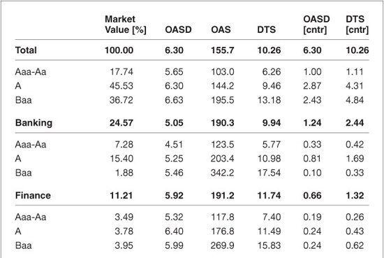
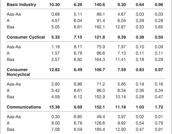
To construct the two replicating portfolios, we first partition the index into 24 cells (eight sector × three credit ratings).²⁰ We then select 10 bonds to represent each cell in the portfolio.²¹ This same set of 10 bonds is used in both variants of the replicating portfolio, to reduce noise from issuer selection and focus attention on the differences in systematic risk exposures. The key difference is in how we weight the bonds within each cell: in the DTS-based portfolio, we match the DTS exposure of the index in each cell, while in the spread-duration-based portfolio we match the index spread duration exposure.²² For example, Exhibit 55–7 shows a market structure report of the Barclays Capital U.S. Corporate Index along the sector/quality partition used for this replication exercise. For each cell of the partition, the report characterizes the exposure of the index to that market segment in three different ways: by market weight, contribution to option-adjusted spread duration (OASD), and contribution to DTS. The spread-duration–based replicating portfolio is constructed such that it matches the contributions to OASD in each of the index sectors (the second column from the right); the DTS-based replication matches the DTS contributions in the rightmost column.

EXHIBIT 55–7
Sector/Quality Profile of Barclays Capital U.S. Corporate Bond Index, as of 12/31/2010

A key part of any index replication attempt is selecting the bonds that form the replicating portfolio. In a real-life portfolio management setting, security selection plays an important role in determining performance and several different criteria can be employed in the security selection process, depending on the portfolio setting. If minimizing tracking error is the primary goal, then the security weights within each cell should focus on the primary issuer exposures of the benchmark. Additionally, managers may aim to maximize liquidity, or to add value by choosing securities that they believe will outperform. Ideally, though, as long as the portfolio has matched the benchmark allocations on the macro level, it should track well in the event of any major industry rally or decline. The key is to match the right set of macro exposures.

For the purposes of this study, our interest is not in the issuer selection mechanism, but in checking which set of macro exposures is most important to match. The selection mechanism therefore does not need to be optimal in any sense (e.g., minimizing tracking error volatility or maximizing performance). Rather, we would like to test our replication methods using several different issuer selection mechanisms, to ensure that differences between the two replicating portfolios (DTS-matched and spread duration matched) are independent of the specific bonds that were selected. One approach is simulation, in which bonds in each cell would be randomly selected, the replication results recorded, and the analysis repeated multiple times. Another approach, which we use instead, is to specify explicit selection criteria based on bond characteristics. While this approach leads to a single replicating portfolio (per criterion), it more closely mimics a realistic process of constructing replicating portfolios for index tracking purposes.

We analyze five potential bond selection criteria. The first criterion, based on market value, selects 10 of the largest bonds in each cell. Hence, it results in the most investible and liquid portfolios (as larger size is generally associated with increased liquidity). The remaining four criteria are designed primarily to maximize our ability to distinguish between the two replication strategies. The second and third criteria rely on spread and select the bonds with the highest (lowest) level of spread. This represents a replication strategy that tries to maximize carry (minimize risk). The last two criteria use an algorithm designed to maximize the dispersion in either spread duration or DTS among the bonds selected within each cell. Selecting bonds with the maximum potential dispersion in the characteristics used to match the index should magnify the mismatch between the portfolio and the benchmark in terms of the exposures not being forced to match. This in turn would facilitate the comparison between the replication results of the two sensitivity measures.

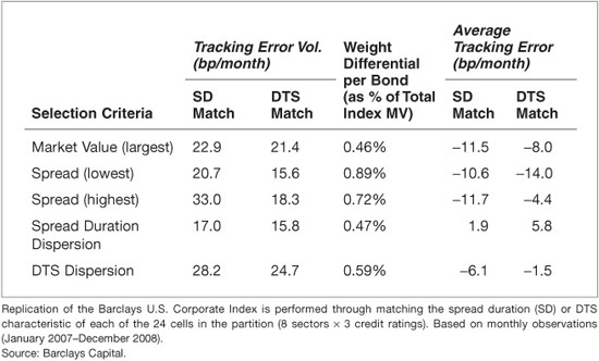
Exhibit 55–8 presents the tracking error volatilities (TEV) of the replicating portfolios during the 24-month period beginning in January 2007, for the various bond selection criteria. Irrespective of the selection criteria, matching each cell’s DTS achieves lower tracking error volatility than matching its spread duration, although the improvement varies widely, from 1.2 bp/month to almost 15 bp/month. Looking at the difference in weight given to each bond under the two matching schemes (reported in the third column) suggests that the reduction in TEV is generally more meaningful as the weight differential increases (i.e., as the replicating portfolios are less similar to each other).²³

For example, if the selection criterion is market value, the average (absolute) difference in the weight of each selected bond under the two replication schemes (in proportion to the total index market value) is 0.46%, and the TEV declines from 22.9 bp/month for matching spread-duration exposures to 21.4 bp/month when matching DTS exposures. If the maximum-spread criterion is used instead, the weight differential rises to 0.72%, and the decline in TEV when matching DTS rather than spread duration exposures is 14.7 bp/month.

It is important to mention that the superior tracking achieved by matching the index DTS does not come at the expense of performance. The last two columns in Exhibit 55–8 display the average tracking errors of the replicating portfolios. The results indicate that while our simple replication exercise tends to underperform the index for any bond selection criteria, the DTS-based approach gives better average tracking errors (with one exception) than the spread duration-based one.

EXHIBIT 55–8
Index Replication Using Stratified Sampling

The use of DTS exposures to replicate an index by stratified sampling is far from a theoretical exercise. This approach has been used to form a highly liquid portfolio of bonds to track the Barclays Capital U.S. Investment-Grade Credit Index.²⁴ A purely rules-driven sampling methodology ensures transparency. The replication methodology uses a partition of five sectors by five duration categories, with each cell represented by two bonds. The bonds are selected based on a proprietary measure of liquidity, and are weighted such that the index DTS exposure in each cell is matched. Historical backtesting of this strategy indicates that it tracks the index much more closely than an alternative strategy based on liquid derivatives including Treasury futures, swaps, and CDX.

EXPRESSING MACRO VIEWS IN ACTIVE PORTFOLIOS

Attention to the DTS exposures of a portfolio is essential for active portfolio managers as well as passive ones. In many financial institutions, the management of a portfolio is a team effort with distinct tasks for different players. Often, one group forms a set of macro views and expresses them as a set of overweights and underweights to various market segments that the portfolio should adopt relative to the benchmark. A second group may be charged with the implementation of this plan in terms of individual securities, often following the issuer selection advice of yet a third group. Yet, in order to achieve the most accurate implementation of the macro views, they must be expressed in terms of the type of exposures that best reflect the way the market moves. Referring back to the index profile shown in Exhibit 55–7, we saw that the passive credit investor will most effectively replicate the macro exposures of the index by matching the DTS contributions in the far right column, not the market value weights or the contributions to OASD. Similarly, the active investor should express the desired overweights and underweights relative to the benchmark in terms of contributions to DTS.

PORTFOLIO CONSTRUCTION: OPTIMAL DIVERSIFICATION OF ISSUER RISK

In the management of all but the most passive credit portfolios, the sizing of credit exposures must find the right balance between two opposing needs. To control risk, it is important to avoid taking a position in any given issuer that is overly concentrated. Conversely, to generate alpha based on analyst recommendations, it is important that the recommended names have sufficient weight in the portfolio to drive outperformance; overemphasis on diversification can dilute the value of issuer selection. As a result, investors often seek guidance on what the “correct” level of diversification should be for a given portfolio.

In the traditional approach to portfolio diversification, a plan sponsor imposes constraints on the portfolio that specify the maximum percentage of the portfolio, by market weight, that may be invested in any single issuer. This issuer limit may be dependent on credit quality, allowing larger concentrations in higher-rated issuers. In the past, we have formulated an approach to optimally determine these quality-dependent limits, based on an empirical study of the performance impact of downgrades.²⁵ This analysis determined that the ratio of allowed position sizes should be based on the relative risks in different quality groups. If the sole concern is downgrade risk, then the ratio indicated based on credit market data gathered from 1988 through 2001 was approximately 9:4:1. This means that if we take the allowed portfolio weight in a Baa-rated issuer as our unit size, a position in a security rated A may be four times as large and positions in Aa-Aaa issuers may be nine times as large. If “natural” spread volatility, which occurs in the absence of a ratings transition, is included in the risk measure as well, the discrepancy between the different ratings categories is lessened, and the ratio becomes 4:3:1. A recent update of this model found that the experience during the 2007–2009 crisis was not supportive of large concentrations even in higher-rated issuers. The same model, updated to include data through the end of 2010, found that the optimal position size ratios were 2.8 : 1.6 : 1 based purely on downgrade risk and 2.6 : 1.6 : 1 when including the effect of all nonsystematic risk, both from downgrades and natural spread volatility.

How can we apply the DTS model to this problem? A first step to this end would be to retain the framework of ratings-dependent caps on issuer market-weight, but compute the position size ratios based on the ratios of average DTS levels in each credit quality group. This approach gives ratios that change over time as spreads widen and tighten, responding quickly to changing market conditions rather than needing to wait for an ex post analysis of realized losses. For example, as of December 2001, the position size ratio from the DTS method was 4.3 : 1.7 : 1, similar to the result from the empirical approach including the risk of both downgrades and natural spread volatility. As market volatility (and spread) ground lower in the following years, these ratios increased, peaking in March 2005 at 6.6 : 3.0 : 1. However, when spreads skyrocketed in 2008, the ratio of position sizes declined, reaching as low as 1.4 : 1.1 : 1 in September 2008, as all credit qualities were deemed highly risky. As of December 2010, the DTS-based ratio of 2.1 : 1.4 : 1 agreed well with that from the updated empirical study.²⁶

However, the DTS paradigm shift suggests a completely different approach to controlling portfolio concentrations, not just a simple recalibration. Rather than imposing a limit on the portfolio market weight in a given issuer (with the size possibly dependent on quality), a limit on the DTS contribution of any issuer should be imposed regardless of credit quality. This would have the effect of allowing a portfolio to have large concentrations in low-spread issuers while enforcing stricter diversification constraints on high-spread issuers. While this idea is attractive in principle, its implementation encounters several practical problems, as we shall discuss.

This DTS-based approach is in some ways quite similar to the traditional approach, in which issuer caps are specified in terms of market weights that differ based on credit quality; yet there are some crucial differences. In both schemes, the fundamental principle is to allow greater concentrations to issuers perceived to be less risky, and require more diversification where risk is greater. The fundamental difference between the two methods is the source of the risk assessment: the quality assigned by the ratings agencies or the spread assigned by the market. There are advantages to each.

Market weight limits based on credit ratings are very well suited for specifying the investment policy for a particular mandate. A permitted position is easy to identify and not subject to debate. Furthermore, as ratings change rather slowly, the guidelines are stable, and the manager is not forced to churn the portfolio as markets move.

Conversely, spreads can react more quickly to market events. As a particular issuer deteriorates in credit quality, the spread-based indicator will typically register that risk has increased much faster than the ratings-based indicator. Nevertheless, while this may be a clear advantage as far as measuring risk, it is not so clear that it is desirable to require managers to transact on price gyrations; the cost of such a policy could be prohibitive. A strict cap on DTS exposure would have the disadvantage of making the limits dependent on pricing, and could lead to inefficient forced selling.

Consider, for example, a strict implementation of a policy that limits DTS contributions. Say we restrict the maximum DTS contribution to any issuer to be 3.0, and that the manager establishes a 0.5% position in issuer XYZ with a spread of 100 bp and a duration of 5 years, for a DTS contribution of 100 × 5 × 0.5% = 2.5. If the spread widens out to above 120 bp, the manager would then be required to sell off some of the position to stay within the limits. This simple example highlights a number of difficulties with this arrangement. First, pricing uncertainty can make it unclear whether a given position is within the guidelines or not. Second, the need to adjust positions as spreads change represents both an undue hardship for managers and an increase in transaction costs for investors.

Another difficulty with a policy based exclusively on DTS contributions is that it can potentially allow very large exposures to short-dated corporates. While the risk of such a position may not be large in terms of spread volatility or excess return volatility, it is clearly undesirable from a tail-risk point of view. A prudent approach to tail risk is to limit the overall portfolio exposure to any single event.

Nevertheless, it is hard to ignore the evidence that credit ratings do not always present the full picture. The broad-brush treatment that allows the same position size for all A-rated issuers, even while large differences in spreads exist across this peer group, clearly leaves room for improvement. There is no question that incorporating information on issuer DTS contributions gives an improvement in our ability to estimate issuer risk. The difficulty is in setting up rules or guidelines that can incorporate this information without requiring unreasonably high turnover. With some ingenuity, it might be possible to reap the benefits of DTS-based risk controls without imposing too much of an operational burden. For example, one could establish a two-tiered constraint with different thresholds for new and existing positions. For instance, in the above example, if the DTS contribution limits were set at 3.0 for new purchases and 4.0 for existing positions, the XYZ position would remain within the guidelines unless the spread widened out from 100 to beyond 160. Presumably, the requirement to reevaluate the exposure to an issuer after a spread move of this magnitude would not be perceived as overly intrusive.

A more difficult challenge for a system of limits on issuer DTS contributions would be a generic rise in corporate spreads, as was seen in 2008. In this crisis environment, it is likely that virtually every issuer in the credit portfolio would exceed the previously established caps on issuer exposures. Would we want to force managers to massively rebalance the portfolio into a market with no liquidity?

In general, forced selling is undesirable, and should be avoided whenever possible. We have conducted empirical studies of the performance impact on corporate bond indices of the forced selling of bonds downgraded to below investment-grade.²⁷ These studies show that investors would be better served by holding on to “fallen angels” well beyond the downgrade, as on average they tend to eventually recoup the overly large losses that they experience as IG managers are forced to sell all at once. How might these results apply to a policy of selling upon a spread widening, even without any change in ratings? This is not at all clear. One might argue that this could help reduce the losses from eventual downgrades; or, conversely, that this would just serve to lock in losses in many bonds that will recover immediately and never suffer a downgrade. Generally, a momentum strategy like this one will do well in trending markets and poorly in choppy markets.

Even when DTS limits are in place, one would probably want to include a hard limit on market value weights, to make sure that no truly large concentrations exist in the portfolio, even in very short-dated or low-spread securities.

In short, we would recommend that for specifying hard limits on issuer exposures within a portfolio mandate, plan sponsors should retain the time-honored tradition of market-weight limits. However, we also believe that managers should track and control the DTS exposures to issuers, and ensure that no single exposure grows too large. Rather than implementing this rule via a hard cutoff beyond which sales would be mandated, managers should have a roughly defined upper limit for issuer DTS exposures, and use their judgment in managing these exposures according to market conditions.

MODELING: CALIBRATING CREDIT-RISK FACTORS

Many portfolio managers rely on multifactor risk models to help them measure and control portfolio risk, either in absolute terms or relative to a benchmark. The DTS approach is ideally suited to estimate spread risk in such models. For example, a risk model might contain modules for measuring exposures to three different types of adverse credit events: systematic changes in spreads, either market-wide or across a particular sector; issuer-specific spread changes; and defaults. The use of DTS can improve the modeling of the first two of these three types of credit risk.

Exposures to systematic changes in credit-spreads in a particular market segment can be measured as the sum of the DTS contributions of all portfolio investments within that segment. The risk factor that relates to these exposures is a relative shift in spreads across the sector; for example, that all financial spreads increase by 10% of their current levels. The alternative to this, in a model not based on DTS, would be to assume that the risk factor is a parallel shift in spreads across a sector (e.g., all financials widen by 10 bp), and that the exposures are therefore contributions to spread duration. Thus, in the DTS-based model, the key risk factor volatility for a particular sector would be its estimated volatility of relative spread changes, as shown in Eq. (55–4) earlier in this chapter, while the alternative model would estimate the volatility of absolute spread changes as per Eq. (55–3).

The DTS-based approach offers three distinct advantages. First, it offers a better assessment of the relative risks of different portfolios. If two portfolios have the same market weight and average spread duration in a given sector, but portfolio A implements this allocation with higher-spread assets than portfolio B, only the DTS-based model will correctly show that portfolio A has a greater exposure to a widening across this sector than does portfolio B. Second, the DTS-based approach improves the accuracy of the risk projection by reducing the uncertainty in the estimation of risk factor volatilities. As we have seen, relative spread volatilities are much more stable than absolute spread volatilities. Therefore, even if we do continually update our estimates of relative spread volatilities within each sector, we find that they change much more slowly than the corresponding estimates of absolute spread volatility and that they are less sensitive to the choice of the time window used in this estimation process.

The third advantage offered by DTS is perhaps more subtle, but opens the door to the most profound change in the structure of the model. Up to this point, we have discussed the exposure to “a given segment of the market” in the abstract, without specifying exactly how the market is to be partitioned. However, choosing the partition along which to measure systematic exposures is one of the most critical elements of risk model design, involving careful tradeoffs among various goals. It is desirable to limit the model to a small number of intuitive factors, both to maximize the clarity and practical applicability of the risk reports produced and ensure that a sufficient number of bonds are available to accurately calibrate each risk factor. Conversely, it is important to include enough factors to achieve sufficient explanatory power. For example, a single risk factor that measures portfolio exposure to U.S. corporates would measure the effect on the portfolio of a potential rally or decline across the corporate bond universe, but not the effect of a relative widening of financials versus industrials. We would like to partition the universe finely enough to capture all major sector rotation effects.

When constructing a model of systematic spread risk for U.S. corporates prior to the introduction of the DTS model, we partitioned this universe into a sector/quality grid, using nine industry groups and three levels of credit ratings for a total of 27 risk factors.²⁸ The partitioning by quality was made absolutely necessary by the assumption that the systematic spread movement in a given market cell tends to take the form of a parallel shift in spreads. When we calibrated such a model to market data, we found that the volatility of absolute spread changes for Baa financials was much greater than that of Aa financials. Although the risk factors representing these two cells might be highly correlated, the substantial difference in volatilities precluded us from combining these cells.

If we instead assume that the spread change across an industry is a relative shift, we find that we no longer need to segregate our model by credit quality. The fact that Baa financials tend to have greater risk than Aa financials is reflected in the higher spreads. This will show up in the risk model as a larger exposure to the same risk factor based on relative spread volatility, rather than as an exposure to a different risk factor with greater (absolute spread) volatility. This puts the risk model designer at a great advantage with regard to the tradeoff between compactness and explanatory power. The model can be designed with roughly the same explanatory power as before using a much smaller number of risk factors, or we can use a finer industry breakdown to create a model with a similar number of factors but greater explanatory power. We have chosen the latter approach in our modeling efforts, increasing the level of sector detail to recognize 27 distinct industry groups.²⁹

KEY POINTS

• Spread volatilities—both systematic and nonsystematic—tend to be proportional to spreads. This empirical observation, with theoretical backing, has many applications to credit portfolio management.

• Forecasts of spread volatility that combine long-term historical estimates of relative spread volatility with current spread levels are more accurate than historical estimates of absolute spread volatility, and are quicker to adapt to changing market conditions.

• Estimates of market beta based on DTS ratios form better projections of future market beta than those based on past observations of empirical market beta.

• Matching index exposures to DTS is a better way to form index-replicating portfolios than matching exposures to market weight or contributions to spread duration. For active managers, credit sector overweights and underweights should be specified and implemented in terms of DTS exposures.

• Measuring and controlling DTS exposures to individual issuers can be viewed as an alternative or a supplement to issuer limits based on market weights and credit qualities.

• Portfolio risk models for fixed income can improve model accuracy and robustness by incorporating the DTS approach to project the risk entailed in both systematic sector overweights and in portfolio concentrations in individual issuers.