CHAPTER
SIXTY-THREE
THE VALUATION OF INTEREST-RATE SWAPS AND SWAPTIONS

GERALD W. BUETOW, JR., PH.D., CFA

Chief Investment Officer
Innealta Capital

BRIAN J. HENDERSON, PH.D., CFA

Assistant Professor of Finance
The George Washington University

An interest-rate swap is an agreement involving two parties who agree to exchange payments at future dates. The cash-flow amounts exchanged in the future are determined by an agreed-upon interest rate and the size, or notional principal, of the agreement. In the most basic interest-rate swap, commonly referred to as a “plain vanilla interest-rate swap,” one party agrees to make variable payments that “float” with a short-term rate while the other party makes fixed-rate payments at an agreed-upon fixed-rate.

Swaps are important tools for risk managers, offering a cost-effective means to altering interest rate exposure. This useful tool for controlling interest rates may be customized in a variety of ways. For example, in an amortizing swap the notional principal declines over time. In an accreting swap, the notional principal increases over time. Other swaps, named forward-start swaps, are swap agreements that commence at a specified date in the future. Another variation of the swap agreement is the basis swap that involves the exchange of payments referencing two different interest rates, such as three-month LIBOR and the three-month Treasury bill.

In this chapter, our focus is on more complex swap structures. We assume the reader is familiar with plain vanilla swaps and the traditional valuation method involving the use of implied forward rates from LIBOR futures contracts to value a swap agreement to compute the swap fixed-rate (SFR). In addition to swaps, we cover the valuation of swaptions. A swaption gives its owner the right to enter into a swap agreement at a future time.

Unlike plain vanilla interest-rate swaps, swaptions have cash flows that depend on an interest rate at a future point in time. This feature requires a versatile approach to valuation. The lattice approach to valuation proves useful due to two important features. First, the interest-rate model driving the lattice approach is fit to no-arbitrage conditions, meaning that the pricing fits the arbitrage values for cash flows using forward rates. Second, the interest-rate models behind the interest-rate lattice incorporate an assumed interest-rate volatility, enabling this approach to handle option-like features.

The balance of the chapter proceeds as follows. We begin by illustrating the lattice approach to valuation with a plain vanilla interest-rate swap. Next, we demonstrate the versatility of the lattice approach through the valuation of forward-start swaps. The chapter proceeds by presenting and pricing swaptions with a focus on the pricing impact of the important parameters (time-to-expiration, strike rate, and volatility). Next, the chapter presents basis swaps and concludes.

SWAP VALUATION USING THE LATTICE APPROACH

The traditional approach to valuing swaps involves obtaining a no-arbitrage value for the swap cash flows by discounting at the implied forward rates. The implied forward rates come from market prices of Eurodollar futures contracts. Unfortunately the traditional approach is not equipped for valuing cash flows that vary depending on interest rates in the future. For this purpose, the lattice model is a useful tool for valuing interest rate derivative instruments such as swaps and swaptions. In contrast to the traditional approach to valuing swaps, the lattice model incorporates the volatility of interest rates to consider how interest rates may change in the future, providing a flexible valuation framework easily adapted to exotic (non–plain vanilla) instruments.

In general, the lattice approach to valuation begins with the construction of the interest-rate lattice.¹ The values on the interest-rate lattice represent possible interest rates in future periods, describing potential evolutions of interest rates through time. After constructing the interest-rate lattice, the swap cash flows are computed at each “node” on the lattice, resulting in the swap cash-flow lattice. The interest rates from the lattice are then used to compute the present value of the possible future cash flows. This process is referred to as backwardation: working backward through the tree to discount the expected future cash flows to a present value.

Constructing the interest-rate lattice begins with an interest-rate model to describe the dynamics of interest rates through time. Although many interest-rate models are used by practitioners, the most common models are one-factor models that describe the evolution of the short rate (one period interest rate) through time. The term one factor simply means that the short rate is the only interest rate being modeled and it solely determines the term structure. An interest-rate model makes important assumptions about the relationship between short-term interest rates and interest-rate volatility, typically measured as the standard deviation.² The examples in this chapter employ a version of the Kalotay, Williams, and Fabozzi interest-rate model.³

After selecting an interest-rate model to describe the possible evolution of the interest rate through time, it is useful to express that model in a lattice comprising discrete time periods. Each node on the binomial tree represents a possible short rate over that discrete time step. The interest rate may evolve to the next time step by taking two possible values. There are other models allowing for more than two possible rates in each subsequent period; for example, the trinomial model allows for three rates. To avoid complication, we illustrate the lattice valuation procedure using the binomial model. The important feature of the interest-rate models is that they satisfy the “no-arbitrage” condition, meaning the interest rates they produce match the implied spot rates from bond prices. Additionally, interest-rate models incorporate an assumption regarding interest-rate volatility. The volatility of interest rates is a critical component when valuing interest rate contingent claims since the cash flows to the claim are determined by interest rates in the future. We will see later that the volatility assumption has direct effects on the value of swaptions.

To illustrate the lattice model approach to valuation, we begin by pricing a 5-year plain vanilla interest-rate swap with a swap fixed-rate (SFR) of 3%. To simplify the presentation, and without loss of generality, we consider the swap to have semiannual payments instead of quarterly payments.

Exhibit 63–1 presents the interest-rate lattice that will be used in the valuation process. The model is a one-factor model and describes the possible paths of the short rate (one-period interest rate) through time. The current short rate is 0.3850%, and according to the model, the short rate for the next time period will be either 0.7950% or 0.6902%, where each of these values is equally likely. The interest-rate tree has 10 semiannual time periods, covering the five-year tenor of the swap agreement.

EXHIBIT 63–1
Interest-Rate Tree

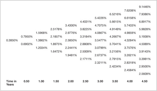
The next step in the valuation process is to compute the cash-flow at each node. The swap payments occur in arrears, but are determined at the start of the period. For instance, the first swap payment is determined today, at t = 0, and is based on the current short rate of interest. Referring to Exhibit 63–1, the current rate is 0.3850%. At the end of the first period, the swap counterparty making the fixed-rate payment will make a payment of:

Fixed-Rate Payment = SFR × NP × (Days in Period / 360)

where NP is the notional principal and Days in Period is the number of days in the payment period.

To simplify the presentation, we assume semiannual cash flows and that the fraction of the year is 0.5. The other swap counterparty, the floating-rate payer, makes a payment that is equal to:

Floating-Rate Payment = Floating-Rate × NP × (Days in Period / 360)

Since the swap cash flows are typically netted, the swap cash-flow at the end of the period will be:

Net Cash-Flow = (Floating-Rate – SFR) × NP × (Days in Period / 360)

Note that when the periodic floating-rate is greater than the SFR, the floating-rate payer makes the net cash-flow payment to the fixed-rate payer. Conversely, when the periodic floating-rate is less than the SFR, the fixed-rate payer makes payment of the net cash flow amount to the floating-rate payer. Exhibit 63–2 presents the net cash flows at each node on the lattice in Exhibit 63–1 for the five-year semiannual swap agreement with a SFR of 3% and notional principal of $100. To illustrate the computation, refer to the node on the upper right hand side of the interest-rate lattice in Exhibit 63–1 where the short rate is 9.1446% at time 4.5 years. At that node, the short rate is 9.1446%. Recall the cash-flow is determined at the start of the period but paid in arrears. Thus, the short rate at time 4.5 years determines the cash-flow at t = 5 years. The net cash-flow from the swap is:

EXHIBIT 63–2
Cash Flow Lattice Illustration; 5-Year Plain-Vanilla Swap, Semiannual Settlement, $100 Notional Principal, SFR = 3%

Net Cash-Flow = (Floating-Rate – SFR) × NP × (Days in Period / 360)

= (9.1446% – 3.0%) × 100 × 0.5 = 3.0723.

The procedure repeats for each node on the tree. Recall that the cash flows to the swap occur in arrears (at the end of the period) but are determined at the beginning of the period based on the interest rate at that time.

At this point in the valuation process, we have used the interest-rate lattice to compute the swap cash flows at each node on the lattice. To arrive at a value for the interest-rate swap, the next step is to construct another lattice referred to as the cumulative swap valuation lattice. Each node of the cumulative swap valuation lattice is the present value of the swap cash flows from all nodes on the cash-flow lattice occurring after that time (see Exhibit 63–2) discounted using the rates on the binomial lattice (see Exhibit 63–1). To illustrate the process, refer to the shaded region in the top right portion of Exhibit 63–3. The cumulative swap valuation at the nodes where t = 4.5 are the present values of the cash flows at t = 5. Note the time reference here – cash flows (t = 5) verse present value of cash flows (t = 4.5). Since the swap agreement matures at t = 5 years, there are no subsequent cash flows to consider. Thus, the values in the shaded region at t = 4.5 years are computed as the present values of the t = 5 cash flows (see Exhibit 63–3) discounted at the rates in Exhibit 63–1:

EXHIBIT 63–3
Cumulative Swap Valuation Lattice; 5-Year Plain-Vanilla Swap, Semiannual Settlement, $100 Notional Principal, SFR = 3%

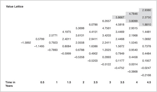
3.0723 / (1 + 9.1446% / 2) = 2.9380

2.4693 / (1 + 7.9386% / 2) = 2.3750

1.9458 / (1 + 6.8917% / 2) = 1.8810.

Working backward to the next time step (t = 4) requires discounting the values at t = 4.5 plus the arrears cash-flow that take place at t = 4.5. At each node, there are two possible values at the next time step and they are equally likely to occur. To illustrate, the values at the shaded t = 4 nodes in Exhibit 63–3 are determined as:

(0.5 × 2.9380 + 0.5 × 2.3750 + 2.3104) / (1 + 7.6208% / 2) = 4.7846

(0.5 × 2.3750 + 0.5 × 1.8810 + 1.8079) / (1 + 6.6158% / 2) = 3.8099.

After computing the cumulative swap values at t = 4, backwardation continues by computing the values at t = 3.5 years. To illustrate, the shaded value in Exhibit 63–3 at t = 3.5 is computed as the present value of the nodes at t = 4 plus the arrears cash-flow received at t = 4:

(0.5 × 4.7846 + 0.5 × 3.8099 + 1.7608) / (1 + 6.5216% /2) = 5.8667.

The process continues through each node, arriving finally at the present value of the swap. Referring to Exhibit 63–3, the present value of the swap with $100 notional principal, 3% swap fixed-rate, and 5-year tenor is −1.5892. Recall that we computed the cash flows from the perspective of the fixed-rate payer, meaning that the cash-flow is negative (an outflow) when the floating-rate is less than the swap fixed-rate. Thus, the negative value indicates that the present value of the fixed-rate payments (3% SFR) is greater than the present value of receiving the floating-rate payments. At the time the counterparties enter into a plain vanilla swap, the present value is zero, meaning the SFR can be determined in the lattice model by iterating on the SFR until the present value at t = 0 of the cumulative swap valuation line equals zero. In this example, a SFR of 2.6650% results in the initial value of the swap equaling zero, illustrating why the swap value is negative to the fixedrate payer in the example where the SFR is 3%. Interest rates must have declined since the inception of the SFR 3% plain vanilla swap.

It is important to note that the value of the plain vanilla swap obtained through the lattice model is identical to the value obtained through the traditional valuation method. This equivalence is due to the fact that the interest-rate model is derived through no-arbitrage conditions based on forward rates determined by market data. The key advantage to the lattice approach will be clear in later sections when we value interest-rate swaptions and need to account for volatility in the possible paths of future interest rates.

Now that we have introduced the binomial lattice, we proceed by introducing more complicated swap structures and swaptions.

FORWARD-START SWAPS

A forward start swap is a swap agreement commencing at some specified date in the future. An example is a two-year swap that begins three years from today. We refer to a forward start swap by the date at which the swap begins and the maturity date of the swap using the notation (y_start, y_end). Thus, the two-year swap beginning three years from today is denoted (3,5). In addition to the start date and maturity date, the forward start swap agreement also specifies the swap fixed-rate and the notional principal. The swap fixed-rate for a forward start swap is referred to as the forward swap fixed-rate.

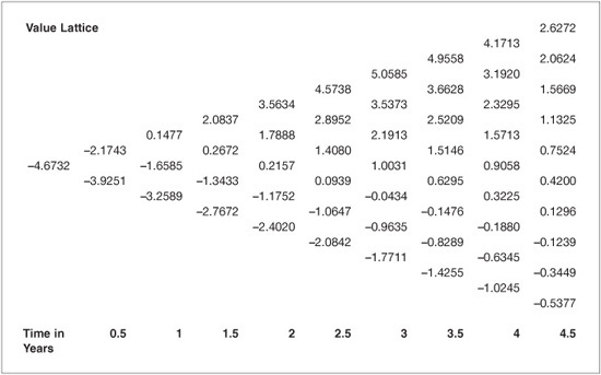
To illustrate the valuation of a forward start swap, we will use the interest-rate lattice presented in Exhibit 63–1 to value the two-year swap that begins three years from today with a fixed-rate of 3.250% and notional principal of 100. The process begins by calculating the swap cash flows at each node on the interest-rate lattice and then constructing the cumulative valuation lattice through the process outlined in the previous section. Exhibit 63–4 presents the cumulative valuation lattice for this swap. Note that the swap begins three years from today and the possible values at time t = 3 years are highlighted in the lattice.

EXHIBIT 63–4
Cumulative Swap Valuation Lattice for (3,5) Forward-Start Swaps, SFR = 3.250%

The cumulative value lattice produces seven possible values for the forward start swap at t = 3 years, and these values can be used to determine the value of the swap agreement. At this point, the missing link is the probability of each of the possible lattice values. The probability of reaching any node in the tree is determined by the number of paths through the lattice that arrive at that node. In the binomial lattice, where there are two possible movements for the rate in the next period, the following formula can be used to calculate the number of paths arriving at any given node:

where n is the number of periods and j is the number of down-states. Exhibit 63–5 presents the number of paths arriving at each node. By referring to the paths at time 3 in the tree, we illustrate the computation using the above formula. Since time on the tree at t = 3 corresponds to the sixth semiannual time step, n = 6. At the very top node, there are no down nodes so j = 0. Evaluating the formula, we find that the number of paths arriving at the top node is 6!/(0!(6!)) = 1 path, which makes sense since the one and only path arriving at the top node consists solely of up-movements. At the node that is second from the top at t = 3, the time periods are still 6 but at this node there is one down-step so j = 1. Evaluating the formula, there are 6!/(1!(5!)) = 6 possible paths arriving at this node.

EXHIBIT 63–5
The Number of Paths Arriving at Each Lattice Node

To finish the demonstration, we compute the number of nodes at the third node from the top at t = 3. At this node, n = 6 and there are two down nodes so j = 2. Applying the formula, the number of paths arriving at the third node are 6!/(2!(4!)) = 15 paths.

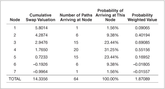
Across the six nodes at t = 3, there are a total of 64 possible paths. The probability of arriving at each node is simply the number of paths to that node divided by the number of possible paths arriving at all nodes at this time. The value of the forward start swap is determined by weighting each of the cumulative swap valuation nodes corresponding to the forward start swap start date by the probability of arriving at that node. This calculation is illustrated in Exhibit 63–6, which presents the seven nodes at t = 3 and the corresponding cumulative swap valuation from the t = 3 node in Exhibit 63–5. The probability of arriving at each node is computed as the number of paths arriving at that node divided by the total number of paths arriving at any node at this time. The product of the cumulative swap valuation and the probability result in the probability weighted value. Summing the probability weighted values results in the forward start swap value. In this case, the value for 100 notional principal of the (3,5) forward start swap with a 3.250% forward start fixed-rate is 1.87089. Note that this is the value to the fixed-rate payer. Recall that we computed the cash flows at each node as the rate on the interest-rate lattice minus the swap fixed-rate. Thus, the positive value indicates that the value of the floating-rate payments exceeds the value of the fixed-rate payments, implying a positive value to the fixed-rate payer. The value to this swap for the floating-rate swap payer is the negative of this amount, −1.87089. The SFR that would produce an FSS value of zero is 4.233% and is computed in the same manner as the iterative routine used to compute the SFR of a zero value plain vanilla swap.

EXHIBIT 63–6
Calculation of the Probability Weighted Value for Year 3

Once we understand the process, we can value forward-start swaps with the same SFR that begin at each node on the lattice and end at five years. That is to say we may compute the values of the otherwise identical (0,5), (0.5,5), (1,5), (1.5,5), (2,5), (2.5,5), (3.5,5), (4,5), and (4.5,5) swaps. Exhibit 63–7 illustrates the computation of forward start swap values at each time period on the lattice.

EXHIBIT 63–7
Probability Weighted Cumulative Valuation Swap Values (SFR = 3.250%, 100 Notional Principal, Maturing in Five Years) and Value of Forward-Start Swaps

VALUING SWAPTIONS

A swaption is an option contract on an interest-rate swap. The owner of a swaption has the right to initiate a swap agreement on or by a specified future date. The swaption specifies several important features of the swap, including the tenor of the swap and the swap fixed-rate. The swap fixed-rate is the strike rate for the option. Unlike a forward start swap, where both counterparties have the obligation to participate in the swap, the swaption owner has the right, but not the obligation, to enter into the swap. We will demonstrate the valuation procedure for swaptions using the interest-rate lattice and discuss how the important parameters affect the swaption valuation.

A payer’s swaption (a pay fixed swaption) gives the owner the right to enter into an interest-rate swap as the fixed-rate payer and receive floating-rate payments. Swaptions may be either European or American style. The difference is that the owner of a European style swaption may exercise their right to enter into the swap at the expiration of the swaption, while the owner of an American style swaption may exercise that right any time up to the expiration date. For our purposes, we will consider European style swaptions.

A receiver’s swaption (receive fixed swaption) givers the owner the right to enter into an interest-rate swap as the floating-rate payer and fixed-rate receiver. As an example, consider a swaption with a fixed-rate of 3.650%, option expiration date of two years, and the swap tenor is three years. The buyer of this swaption has the right at the end of two years to enter into a swap in which they make floating-rate payments and receive fixed-rate payments of 3.650%. We introduce the notation (y_expiration, y_tenor) for swaptions to refer to the expiration date of the swaption and the tenor of the swap. Thus, the receiver’s swap is a (2,3) swaption.

To illustrate swaption pricing, we will price several payers’ swaps with a strike rate of 3.650%. The lattice approach is helpful to value swaptions, and the valuation example uses the interest-rate lattice from Exhibit 63–1. After constructing the interest-rate lattice, the next step in the valuation process is to construct the pay fixed cash-flow lattice for a plain vanilla swap with a notional principal of $100, based on a swap fixed-rate of 3.650%. Recall that at each node on the lattice, the cash-flow is determined by the swap fixed-rate, the notional principal, the corresponding node on the interest-rate lattice:

Cash-Flow _i,j = (F_i,j−1 − SFR) × NP_j × 0.5

where F_i,j−1 is the floating-rate at node (i,j-1), indicating the arrears cash-flow at time j. Exhibit 63–8 presents the cash-flow lattice for the plain vanilla swap with a strike rate of 3.650%. To illustrate the computation of the cash flows, refer to the top-right node on the tree. Note that this cash-flow occurs at time t = 5, but is determined by the rate at t = 4.5. The corresponding rate from the interest-rate lattice is 9.1446%, so the cash-flow at this node is:

EXHIBIT 63–8
Pay Fixed Cash Flow Lattice for Plain Vanilla Swap (Strike Rate = 3.65%)

Cash-Flow_1,5 = (9.1446% − 3.650%) × 100 × 0.5 = 2.7473

After constructing the cash-flow lattice in Exhibit 63–8, the next step in the swaption valuation process is to construct the cumulative swap valuation lattice for the plain vanilla pay-fixed swaption. Exhibit 63–9 presents the cumulative valuation lattice. The cumulative swap valuation lattice can then be used to value pay fixed swaptions.

EXHIBIT 63–9
Cumulative Swap Valuation Lattices, 5-Year, Semiannual, Plain Vanilla Swap and Strike Rate of 3.65%

To illustrate the swaption valuation, we price the (3,2) pay fixed swaption, as illustrated in Exhibit 63–10. The option expires in year 3 and the values corresponding to expiration are referred to as the expiration values. The expiration value at each node (here t = 3) come from the values in the cumulative valuation lattice (see Exhibit 63–9). Recall that the swaption gives the owner the right, but not the obligation to enter into the pay fixed swap. The owner will only exercise this right when the value of the two-year swap commencing at t = 3 is positive. Thus, the expiration values for the swaption are the maximum of zero or the value at the corresponding node on the cumulative valuation lattice. To illustrate, at the bottom node on the tree at t = 3, the cumulative valuation for the pay-fixed swap is −0.7711. Intuitively, this makes sense since the bottom nodes correspond to low interest rates that adversely affect the fixed-rate payer.

EXHIBIT 63–10
(3,2) Pay Fixed Swaption, Strike Rate 3.65%

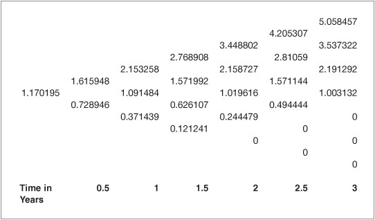
After determining the expiration values for the swaption, the remaining portion of the lattice is populated using backward induction. The corresponding rates from the interest-rate lattice determine the discount factors. To illustrate the process, the top value at year 2.5 in Exhibit 63–10 is computed as:

0.5 (5.058457 + 3.537322) / (1 + 4.4031% / 2) = 4.205307

Repeating this process throughout the lattice in Exhibit 63–10 results in a value of $1.170195 for the (3,2) pay fixed swaption per $100 of notional principal. It is worth noting that the lattice valuation process requires as inputs the interest-rate lattice and the swaps valuation lattice. Once these have been determined, it is straightforward to price any variation of the swaption having the same fixed-rate. The lattice valuation framework is very flexible and handles easily any adjustments such as varying the notional principal (amortizing or accreting). This flexibility makes the lattice approach to valuation attractive.

VALUING BASIS SWAPS AND NON-LIBOR-BASED SWAPS

To this point, we have focused on the valuation of swap structures involving the exchange of floating and fixed-rate payments in which the floating leg of the swap is based off LIBOR. Next, we generalize our discussion to include swaps in which both legs of the swap float and to swap structures based on interest rates other than LIBOR.

A basis swap is a swap agreement in which both legs of the swap are based on different rates. For example, the spread between the 90-day Treasury bill rate and the three-month LIBOR is referred to as the TED spread. In a LIBOR TED swap, one counterparty makes payments based on LIBOR and receives payments based on the 90-day Treasury bill rate plus a spread. This is referred to as a pay LIBOR TED swap.

We illustrate the lattice approach to valuation for a one-year pay LIBOR TED swap with a Spread of 0.376%. Since each leg of the swap references a floating-rate, the lattice approach requires a lattice for each rate. Exhibit 63–11 presents the one-year interest-rate lattices for LIBOR and the 90-day Treasury bill rate. Note that we assume a 10% volatility for LIBOR and 7.5% for the Treasury bill rate. In previous examples, we assumed semiannual periodicity for payments. In this example we assume quarterly.

EXHIBIT 63–11
One-Year Interest-Rate Lattices for LIBOR TED SWAP

After the two interest-rate lattices are in place, the next step in the valuation process is to compute the cash flows for the pay LIBOR TED swap. Each cash-flow at node i in period j is computed as follows. Note that in the example

we ignore the exact day count and assume each period is exactly one quarter of the year.

CF_i,j = (T-Bill_i,j-1 + Spread − LIBOR_i,j-1) × 0.25 × NP_j

It is important to point out that the Spread is the adjustment to the Treasury bill rate such that the present values of the two payment streams are equal. To obtain the spread that equates the two cash-flow streams, we can iterate on the Spread value.

Following the two interest-rate lattices in Exhibit 63–11, the next step is the computation of the pay LIBOR TED swap cash flow at each node on the tree. To illustrate, consider the highest node on the tree at maturity of the swap. Referring to Exhibit 63–11, the LIBOR and Treasury bill rate at this node are 1.01% and 0.29%, respectively. Using the Spread of 0.376%, the payment on $100 notional principal is:

CF_i,j = (T-Bill_i,j-1 + Spread − LIBOR_i,j-1) × 0.25 × NP _j

= (0.29% + 0.376% – 1.01%) × 0.25 × NP _j

= –0.085

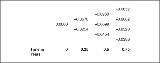
The cash flows for the swap at all times are presented in Exhibit 63–12. After constructing the cash flows, the final step for valuing the pay LIBOR TED swap is to compute the cumulative value lattice. This procedure is exactly the same as demonstrated in previous sections. The values are presented in Exhibit 63–13. Note that the present value of the expected payments is zero, indicating that the spread of 0.376% produces zero value for the swap. This means the present value of the LIBOR and the Treasury bill plus spread legs are identical. For Spreads greater (smaller) than 0.376%, in this example the pay LIBOR TED swap would have positive (negative) present value. To note the flexibility of the lattice approach to valuation, note that it is straightforward to extend the valuation for a swaption on a basis swap following the procedure outlined in the previous section.

EXHIBIT 63–12
Cash Flows for Pay LIBOR TED Swap, Spread of 0.376%

EXHIBIT 63–13
Cumulative Value Lattice for Pay LIBOR TED Swap, Spread of 0.376%

FACTORS AFFECTING SWAP VALUATION

The flexibility of the lattice approach to valuation facilitates the analysis of a swaption’s sensitivity to changes in the swaption terms and changes in market inputs such as volatility. In this section, we illustrate the sensitivity of swaption valuations to interest-rate volatility and the strike rate.

There are two main determinants of the values in the interest-rate lattice: the current term structure and interest-rate volatility. Recall that the interest-rate lattice is the basic building block in the lattice approach to valuing swaptions. Changing the expiration date of a swap changes the value of the swaption, but the directional change in value depends on the current term structure, volatility, and strike price. Interest-rate volatility, however, increases the value of swaptions, holding all else constant.

The chart in Exhibit 63–14 illustrates the effect of interest-rate volatility and the expiration of the swap on the valuation of four different pay fixed swaptions. To construct the example, we use the LIBOR interest-rate lattice from Exhibit 63–1 and consider pay-fixed swaptions each having a strike rate equal to 3.5%. In the figure, there is not a monotonic relation between the swaption expiration and value. Each swaption’s value, however, does increase as volatility increases.

We next consider the joint effect of the strike rate and interest-rate volatility on interest-rate swaptions. Exhibit 63–14 illustrates that swaption values increase as interest-rate volatility increases, holding all else constant. The strike rate has an important impact on the value of the swaption. For a pay fixed swaption, in which the option owner has the right to enter into a swap agreement where they pay the fixed-rate and receive floating payments, as the strike rate increases, the value of the pay fixed swaption declines since the value of the fixed-rate payments rises relative to the floating-rate payments that party will receive. Conversely, in a receive fixed swaption, in which the option owner has the right to enter into a swap agreement where they receive fixed-rate payments and make floating-rate payments, the value of that right increases as the strike rate increases.

EXHIBIT 63–14
Pay Fixed Swaption Values and Volatility, Strike Rate = 3.5%

Exhibit 63–15 illustrates the joint effect of the strike rate and interest-rate volatility on the value of a (2,3) pay fixed swaption. The surface plot of the swaption value is increasing in the volatility (at higher levels of volatility, the swaption’s value is greater), and decreasing in the strike rate (at lower strike rates, the pay-fixed swaption’s value is greater). Exhibit 63–16 illustrates the receive fixed swaption value across strike rates and levels of volatility. It is important to note that, across the strike rate dimension, the graph in Exhibit 63–16 is the mirror image of Exhibit 63–15, demonstrating that strike rate has the opposite impact on the values of receive fixed swaptions as it has on pay fixed options. The value of the receiver’s swaption, is positively related to the level of volatility, in which the receiver’s swaption increases in value as the assumed lever of interest-rate volatility increases.

EXHIBIT 63–15
The Effect of Strike Rate and Interest-Rate Volatility on the (2,3) Pay Fixed Value

EXHIBIT 63–16
The Effect of Strike Rate and Interest-Rate Volatility on the (2,3) Receive Fixed Swaption Value

KEY POINTS

• Interest-rate swap agreements involve two parties agreeing to exchange payments in the future at agreed-upon terms.

• Exotic swap agreements are customized contracts. Common variations include forward-start swaps, amortizing notional principal swaps, accreting notional principal swaps, basis swaps, and non-LIBOR swaps.

• Swaptions are option contracts in which the owner has the right, but not the obligation, to enter into a swap agreement in the future.

• The lattice approach to swap and swaption valuation is a powerful, flexible valuation framework easily adapted to handle variations of exotic swaps.

• Swaption values are determined by market inputs such as the term structure of interest rates and interest-rate volatility in addition to contract specifications such as tenor and strike rate. Holding all else constant, volatility increases swaption values. Holding all else constant, increasing the strike rate decreases the value of a pay-fixed swaption but increases the value of a receive-fixed contract.