Our purpose in this chapter is to introduce the idea of orientation frames in two dimensions, and in particular to study the technology of moving orientation frames. We choose two dimensions as our logical starting point because it is the simplest framework available, and there are many basic concepts that generalize to three dimensions and provide insight into quaternion methods.
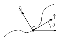
Suppose we have a 2D object (a simple box, for example), as shown in Figure 19.1. The orientation frame consists of two orthogonal vectors, denoted by the tangent T (the direction corresponding to the slope of the “hillside” the box is sitting on) and the normal N, which is the direction perpendicular to the “hillside” curve and perpendicular to the direction of T. This simple example will allow us to study the following two profound concepts:
Basic fact 1: The columns of any rotation matrix are interpretable as coordinate frame axes.
Basic fact 2: Rotation matrices belong to a group, and because groups have geometric properties each matrix is actually a point on a geometric object. Therefore, any set of coordinate frame axes is also such a point.

Figure 19.1. Moving frame on a smooth curve defined by the tangent and normal directions. The pair ![]() is a rotation matrix defining the relation of the curve’s tangent frame to the orientation described by the 2 × 2 identity matrix.
is a rotation matrix defining the relation of the curve’s tangent frame to the orientation described by the 2 × 2 identity matrix.
We will now begin the task of more deeply understanding rotations, their associated coordinate frame axes, and the phenomenon of moving frames in 2D. We will continue to find new ways to exploit the fact that there exists a geometric correspondence between rotations and the geometry of complex numbers. Because complex numbers are a special subspace of quaternions, 2D rotations can be used to introduce us to quaternion frames and their geometric meaning.
The first visualization of a rotation matrix we will use is based on the idea of a smooth curve in the plane, as shown in Figure 19.1. At each point of the curve, we can see that there is a tangent vector. We will let one end of the curve be the “beginning,” so that the tangent vector points unambiguously from the beginning toward the end. In precise mathematical terms, if the curve is specified by a pair of parametric functions, which we write as the two-vector
f(t) = (x(t), y(t)), |
the tangent vector at each point of the curve is the derivative
The reader should be convinced that this derivative and the slope of the curve are the same thing. (Hint: Try some simple examples, such as f(t) = (t, 0), f(t) = (t,t), f(t) = (t,t3), and so on.)
We take the convention that if the direction T is the “virtual x axis” of a 2D coordinate frame there is a unique “virtual y axis” dictated by the right-handed orientation convention. We call this the normal direction and denote it by
Clearly, T(t) · N(t) = 0 for all t, and therefore the tangent and the normal together can be normalized to form an orthonormal moving frame:
The tangent and normal change continuously as we move along the 2D curve, as implied by Figure 19.1.
The varying orientation of the frame is described at each point (or time) by the 2D rotation matrix
as well as the two more abstract forms we have already introduced,
(with the constraint A2+ B2 = 1) and
with the constraint a2 + b2 = 1.
Next let us examine the time evolution of the 2D frame, which will be of great interest in 3D. First, using the coordinates θ (t) for the frame we have
Differentiating the columns separately, we find the frame equations
where κ(t) = dθ/dt is the curvature.
This is the 2D analog of the 3D Parallel Transport Frame, which handily maps any continuously differentiable curve into its corresponding tangent frame. The set of Equations 19.3 is often arranged to make a “vector matrix equation:”
We are going to start studying objects by creating new objects that are closely related to them, usually with a point-by-point correspondence, but which may not correspond exactly to the objects themselves. This approach is known as a map. Creating a map amounts to taking a point p on a geometric object and giving a rule that tells us how to compute a new point x that is not necessarily even of the same dimension as p. Formally, we might write
f | maps p → x, |
f(p) | = x, |
with typical examples being, respectively, the constant map, a scalar field, the identity map, or a tensor map:
f(p) = 1,
f(p) = p,
f(p) = pipj,
The task of the map f(p) is to perform some computation depending on the point p and to return some object, possibly a vector of the same dimensions, possibly not, that is related to each point p.
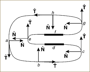
In Figure 19.2, we show an example of a 2D curve with its tangent and normal fields. The normalized tangent and normal fields have only one degree of freedom, which we denote by the angle θ(t). The column vectors ![]() and
and ![]() then represent a moving orthonormal coordinate frame, as in Equation 19.2.
then represent a moving orthonormal coordinate frame, as in Equation 19.2.

Figure 19.2. A smooth 2D curve with its normal and tangent frame fields. The segments d and f are intended to be straight.
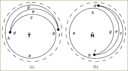
A 2D version of the Gauss map [46,61] used in the classical differential geometry of surfaces follows when we discard the original curve (Figure 19.2) and restrict our view to show only the path of the normalized tangents (as in Figure 19.3a) or the normalized normals, as in Figure 19.3b. Both vector fields take values only in the unit circle. These are the tangent map of the curve in Figure 19.2, and the normal map of the curve in Figure 19.2, respectively.

Figure 19.3. 2D Gauss map sketches of (a) the tangent directions and (b) the normal directions corresponding to the U-shaped curve shown in Figure 19.2. All vectors lie on the unit circle in 2D. The straight line segments along d and f in Figure 19.2 correspond to single points in both maps.
We note that any sufficiently small open neighborhood of the curve has unique tangent and normal directions, up to the possibility of a shared limit point for straight segments such as d and f (Figure 19.2). Over the entire curve, however, particular neighborhoods of directions may be repeated many times, resulting in an overlapping nonunique 2D map, as indicated schematically in Figure 19.3. We will accept this as a feature, not necessarily a deficiency, of the construction.
With some amount of prescience about quaternions, we can ask what happens if we express the standard angular form of the 2D frame equations we have been using not in the form of the (A = cosθ, B = sinθ) variables but in terms of a = cos(θ/2), b = sin(θ/2) (i.e., A = a2 – b2, B = 2ab). When we carry through this alternative parameterization, we find, as usual,
where orthonormality implies (a2 + b2)2 = 1, which reduces back to
a2 + b2 = 1. |
We observe that the pair (a, b) provides a double-valued parameterization of the frame:
Here, (a, b) describes precisely the same frame as (–a, –b).
Remark: Yet another one-parameter representation. The redundant parameter can be eliminated locally by using projective coordinates such as c = b/a = tan(θ/2), where –∞ < c < + ∞, to get another parameterization:
(Note: there is a useful equivalent of this formula for quaternions.)
Using the basis ![]() for the frame, we have four equations with three constraints from orthonormality, yielding one true degree of freedom. However, a major simplification occurs when we carry out the calculation in (a, b) coordinates! Differentiating, we get
for the frame, we have four equations with three constraints from orthonormality, yielding one true degree of freedom. However, a major simplification occurs when we carry out the calculation in (a, b) coordinates! Differentiating, we get
However, this formula for ![]() is just κ
is just κ![]() , where
, where
or
Now, because
is an orthogonal matrix, we can simply multiply the pair of equations for ![]() and
and ![]() by the transpose, so that
by the transpose, so that ![]() becomes precisely equivalent to
becomes precisely equivalent to
Thus, (a(t), b(t)) with the constraint a2 + b2 = 1 acts as the square root of ![]() and the differential equation given by Equation 19.6 contains all properties needed to compute and reconstruct the behavior of the frame described in a less elegant way by Equations 19.3 and 19.4.
and the differential equation given by Equation 19.6 contains all properties needed to compute and reconstruct the behavior of the frame described in a less elegant way by Equations 19.3 and 19.4.

