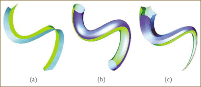
The methods of 3D frames are taught as a basic area of study in differential geometry. However, classical methods do not take advantage of the quaternion techniques that can be used to clarify the nature of moving frames. In this chapter we review the classical differential geometry of moving frames on 3D space curves, and then introduce the equivalent quaternion formulation along with the quaternion tangent map, which allows us to see global properties of a framing choice at a single glance.
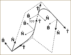
The fundamental difference between 2D space curves and 3D space curves is that although the tangent direction is still determinable directly from the space curve, there is an additional degree of rotational freedom in the normal plane, the portion of the frame perpendicular to the tangent vector. This is indicated schematically in Figure 20.1.

Figure 20.1. General form of a moving frame for a 3D curve x(t), with the tangent direction ![]() determined directly from the curve derivative and the exact orientation of the basis
determined directly from the curve derivative and the exact orientation of the basis ![]() for the normal plane determined only up to an axial rotation about
for the normal plane determined only up to an axial rotation about ![]() .
.
Dense families of space curves can be generated by many applications, including time-dependent particle flow fields, static streamlines generated by integrating a volume vector field, and deformations of a solid coordinate grid. Our fundamental approach singles out space curves, although variations could be used to treat individual point frames (see Alpern et al. [3]), stream surfaces (see Hultquist [99]), and orientation differences (which are themselves orientation fields). Thus, we begin with the properties of a curve x(t) in 3D space parameterized by the unnormalized arc length t. If x(t) is once-differentiable, the normalized tangent vector at any point is
The standard arc-length differential is typically expressed as
In practice, we never have smooth curves in numerical applications, but only piecewise linear curves that are presumed to be approximations to differentiable curves. Thus, for a curve given by the set of points {xi} we might typically take
or any corresponding formula with additional sampling points and desirable symmetries. We would typically use a five-point formula to get a smoother result. One could also produce finer intermediate states by spline interpolation.
If the curve is locally straight—that is, x″(t) = 0 or ![]() —there is no locally determinable coordinate frame component in the plane normal to
—there is no locally determinable coordinate frame component in the plane normal to ![]() . A nonlocal definition must be used to decide on the remainder of the frame once
. A nonlocal definition must be used to decide on the remainder of the frame once ![]() is determined. In the following, we formulate our two alternate coordinate frames, one of which (the Frenet frame) is completely local but is indeterminable where the curve is locally straight. The other coordinate frame, the parallel transport frame, is defined everywhere but depends on a numerical integration over the entire curve.
is determined. In the following, we formulate our two alternate coordinate frames, one of which (the Frenet frame) is completely local but is indeterminable where the curve is locally straight. The other coordinate frame, the parallel transport frame, is defined everywhere but depends on a numerical integration over the entire curve.
Tangent map examples: The tangent direction of a 3D curve at each point is given simply by taking the algebraic or numerical derivative of the curve at each sample point and normalizing the result. Each tangent direction thus has two degrees of freedom and lies on the surface of the two-sphere S2. The curve resulting from joining the ends of neighboring tangents is the tangent map of the curve. As in the 2D case treated earlier, the tangent map of a 3D curve is not necessarily single valued except in local neighborhoods, and may have limit points (e.g., if there are straight segments). In Figures 20.2a and 20.2b we show examples of two classic 3D curves—one a closed knot, the (2, 3) trefoil knot lying on the surface of a torus, and the other the open helix:

Figure 20.2. Tangent maps. (a) The (2, 3) torus knot and the helix as 3D line drawings. (b) Illustrating an application of tubing to make the 3D curves more interpretable. (c) The corresponding normalized tangent maps determined directly from the curve geometry. These are curves on the two-sphere, which have been tubed to improve visibility.
For the torus knot, p and q are normally relatively prime integers, r is the radius of the torus, and a and b describe the elliptical cross section of the toroidal tube. Differentiating these curves yields the tangent maps shown in Figure 20.2c.
The evolution properties of all possible frames for a 3D curve x(t) can be written in a unified framework. The basic idea is to consider an arbitrary frame to be represented in the form of columns of a 3 × 3 orthonormal rotation matrix:
Here, ![]() is the normalized tangent vector determined directly by the curve geometry and is thus unalterable.
is the normalized tangent vector determined directly by the curve geometry and is thus unalterable. ![]() is a pair of orthonormal vectors spanning the plane perpendicular to the tangent vector at each point of the curve. Because
is a pair of orthonormal vectors spanning the plane perpendicular to the tangent vector at each point of the curve. Because ![]() and all other inner products vanish by definition, any change in a basis vector must be orthogonal to itself and thereby expressible in terms of the other two basis vectors. Thus, the most general possible form for the frame evolution equations is
and all other inner products vanish by definition, any change in a basis vector must be orthogonal to itself and thereby expressible in terms of the other two basis vectors. Thus, the most general possible form for the frame evolution equations is
where v(t) = ‖x′(t)‖ is the velocity of the curve if we are not using a unit-speed parameterization. (See Equation 19.4 for comparison.)
The particular choice of notation and signs for the curvatures k in Equation 20.4 is compellingly motivated by the quaternion algebra treatment to be presented later. The natural properties of the curve-frame evolution are also exposed using the Darboux form of the equations
where F generalizes the Darboux vector field (e.g., see Gray [61, p. 205]):
The square magnitude of the total “force” acting on the frame is ![]() , and we will see in the following that this is a minimum for the parallel transport frame. The arbitrariness of the basis
, and we will see in the following that this is a minimum for the parallel transport frame. The arbitrariness of the basis ![]() for the plane perpendicular to
for the plane perpendicular to ![]() can be exploited as desired to eliminate any one of the (kx, ky, kz) (e.g., see Bishop [19]). For example, if
can be exploited as desired to eliminate any one of the (kx, ky, kz) (e.g., see Bishop [19]). For example, if
differentiating and substituting from Equation 20.4 yields
Thus, the angle θ(t) may be chosen to cancel the angular velocity kz in the plane spanned by ![]() and
and ![]() . The same argument holds for any other pair. Attempting to eliminate additional components produces new mixing, leaving at least two independent components in the evolution matrix.
. The same argument holds for any other pair. Attempting to eliminate additional components produces new mixing, leaving at least two independent components in the evolution matrix.
We remark that to generate a ribbon or tube such as those we commonly use to display curves one simply sweeps the chosen set of frames through each curve point p(t) to produce a connected tube:
The resulting structure is sampled in t and over one full 2π period in θ to produce a tessellated tube. Arbitrary functions of (t, θ) can be introduced instead of the cosine and sine to produce ribbons and general linear structures. A typical example of a tube-based modeling operation, sometimes known as the generalized cone, takes a particular 2D cross-section shape and moves it along a framed path, possibly varying in size or shape as it travels. The result is the class of tube-like geometric objects shown in Figure 20.3.
We now note a variety of approaches to assigning frames to an entire 3D space curve, each with its own peculiar advantages. Figure 20.4 compares the tubings of the (2, 3) trefoil knot and the helix for each of the three frames described in the following. For further details, see (for example) Eisenhart [46] and Gray [61].

Figure 20.4. Curve framings for the (2, 3) torus knot and the helix based on (a) Frenet frame, (b) geodesic reference frame (minimal tilt from North Pole), and (c) parallel transport frame, which is not periodic like the other frames.
The classical Frenet–Serret frame, also commonly referred to as the “Frenet frame,” is determined by local conditions at each point of the curve but is undefined whenever the curvature vanishes (e.g., when the curve straightens out or has an inflection point). For the Frenet frame, we make the choices
where κ(t) is the curvature (which geometrically can be understood as the inverse radius of curvature at a curve point) and τ(t) is the torsion, which mixes the two normal vectors in their local plane. This identification produces the Frenet–Serret equations
Note that the squared Darboux vector is thus ‖F‖2 = κ2 + τ2 ≥ κ2.
If x(t) is any thrice-differentiable space curve, we can identify the triad of normalized Frenet frame vectors directly with the local derivatives of the curve,
where one can identify the curvature and torsion in Equation 20.10 with
and
respectively.
We illustrate the standard Frenet frame configuration in Figure 20.5. When the second derivative vanishes on some interval, the Frenet frame is temporarily undefined, as illustrated in Figure 20.6. Attempts to work around this problem involve various heuristics [147] but can be resolved rigorously using the Bishop frame [19], also known as the parallel transport frame, which we will describe in a moment.
The parallel transport frame is equivalent to a heuristic approach that has been frequently used in graphics applications (e.g., see Bloomenthal [21], Klock [114], Max [121], Shani and Ballard [147]). A careful mathematical treatment by Bishop [19] presents its differential properties in a form that can be easily compared with the standard features of the Frenet frame. The parallel transport frame is distinguished by the fact that it uses the smallest possible rotation at each curve sample to align the current tangent vector with the next tangent vector. The current orientation of the plane normal to the tangent vector depends on the history of the curve, starting with an arbitrary initial frame, and thus one is essentially integrating a differential equation for the frame change around the curve. The frame depends on the initial conditions, and unlike the Frenet frame cannot be determined locally on the curve. The algorithm with the best limiting properties [119] for computing this frame involves determining the normal direction ![]() to the plane of two successive tangents to the curve, finding the angle θ = arccos
to the plane of two successive tangents to the curve, finding the angle θ = arccos ![]() and rotating the current frame to the next frame using the 3 × 3,
and rotating the current frame to the next frame using the 3 × 3, ![]() or its corresponding quaternion,
or its corresponding quaternion,
(Recall that we define q(θ, ![]() ) = (cos(θ/2),
) = (cos(θ/2), ![]() sin(θ/2)).) If the successive tangents are collinear, one leaves the frame unchanged. If the tangents are anti-collinear, a result can be returned but it is not uniquely determined. To identify the parallel transport frame with Equation 20.4, we set
sin(θ/2)).) If the successive tangents are collinear, one leaves the frame unchanged. If the tangents are anti-collinear, a result can be returned but it is not uniquely determined. To identify the parallel transport frame with Equation 20.4, we set
ky | ⇒ | k1(t) |
–kx | ⇒ | k2(t) |
kz | ⇒ | 0 |
to avoid unnecessary mixing between the normal components (effectively the definition of parallel transport). This choice produces Bishop’s frame equations:
This frame choice behaves entirely differently from the Frenet frame because, as illustrated in Figure 20.7, it remains continuous and well defined for a curve with vanishing curvature on a segment.
![The parallel transport curve frame for the curve shown in Figure 20.6 [19]. This frame, unlike the Frenet frame shown in Figure 20.6, is continuous along the “roof peak” (where the curvature vanishes).](http://imgdetail.ebookreading.net/design/11/9780120884001/9780120884001__the-morgan-kaufmann__9780120884001__graphics__20fig07.gif)
Figure 20.7. The parallel transport curve frame for the curve shown in Figure 20.6 [19]. This frame, unlike the Frenet frame shown in Figure 20.6, is continuous along the “roof peak” (where the curvature vanishes).
Because ![]() is an invariant independent of the choice of the normal frame, Bishop identifies the curvature, orientation, and angular velocity as
is an invariant independent of the choice of the normal frame, Bishop identifies the curvature, orientation, and angular velocity as
![The parallel transport curve frame for the curve shown in Figure 20.6 [19]. This frame, unlike the Frenet frame shown in Figure 20.6, is continuous along the “roof peak” (where the curvature vanishes).](http://imgdetail.ebookreading.net/design/11/9780120884001/9780120884001__the-morgan-kaufmann__9780120884001__graphics__191equ01.gif)
k1 and k2 thus correspond to a Cartesian coordinate system for the curvature polar coordinates (κ, θ), with θ = θ0 + ∫ ω(t)dt and ω(t) is effectively the classical torsion τ(t) appearing in the Frenet equations. A fundamental ambiguity in the parallel transport frame compared to the Frenet frame thus arises from the arbitrary choice of an integration constant for θ, which disappears from τ due to the differentiation. Note that the squared Darboux vector ![]() is now a frame invariant. It is missing the torsion component present for the Frenet frame, and thus assumes its minimal value.
is now a frame invariant. It is missing the torsion component present for the Frenet frame, and thus assumes its minimal value.
A numerical method of computing the parallel transport frame with the desired properties works as follows. Given a frame at xi–1, compute two neighboring tangents Ti and Ti–1 and their unit vectors ![]() . Find the angle θ = arccos
. Find the angle θ = arccos ![]() between them and find the perpendicular to the plane of the tangents given by
between them and find the perpendicular to the plane of the tangents given by ![]() . Finally, rotate the frame at xi–1 by θ about
. Finally, rotate the frame at xi–1 by θ about ![]() to get the frame at point xi.
to get the frame at point xi.
Just as for the Frenet frame, one can begin with a curve x(t) and an initial frame, or a pair of functions (k1(t), k2(t)) and an initial frame, or a frame over the entire curve, and then integrate where needed to compute the missing variables. It is also worthwhile noting that (k1(t), k2(t)) form a 2D Cartesian vector field at each point of the curve, and thus allow a natural alternate characterization to Gray’s (κ, τ) curve properties [31,60].
We will often need a frame that is guaranteed to have a particular axis in one direction, but we will not care about the remaining axes because they will be considered as a space of possibilities. A convenient frame with these properties can always be constructed starting from the assumption that there exists a canonical reference frame in which, say, the ![]() axis corresponds to the preferred direction. Thus, if
axis corresponds to the preferred direction. Thus, if ![]() is the desired direction of the new axis, we can simply tilt the reference axis
is the desired direction of the new axis, we can simply tilt the reference axis ![]() into
into ![]() along a minimal, geodesic curve using an ordinary rotation R(θ,
along a minimal, geodesic curve using an ordinary rotation R(θ, ![]() ) or its corresponding quaternion:
) or its corresponding quaternion:
Clearly any reference frame, including frames related to the viewing parameters of a moving observer, could be used instead of ![]() . This frame has the drawback that it is ambiguous whenever
. This frame has the drawback that it is ambiguous whenever ![]() = –
= –![]() . Sequences of frames passing through this point will not necessarily be smoothly varying because only a single instance of a one-parameter family of frames can be returned automatically by a context-free algorithm. Luckily, this is of no consequence for most of our applications. As we will discuss later in the quaternion framework, this property is directly related to the absence of a global vector field on the two-sphere.
. Sequences of frames passing through this point will not necessarily be smoothly varying because only a single instance of a one-parameter family of frames can be returned automatically by a context-free algorithm. Luckily, this is of no consequence for most of our applications. As we will discuss later in the quaternion framework, this property is directly related to the absence of a global vector field on the two-sphere.
When possible, we will work with the top-level framework for coordinate frames of arbitrary generality, rather than choosing conventional frames or hybrids of the frames described so far (e.g., see Klock [114]). Although the classical frames have many fundamentally appealing mathematical properties, we are not restricted to the use of any one of them. Keeping the tangent vector field intact, we may modify the angle of rotation about the tangent vector at will to produce an application-dependent frame assignment. An example of such an application is a closed curve with inflection points: the Frenet frame is periodic but not globally defined, the parallel transport frame will not be periodic in general, and the geodesic reference frame will be periodic but may have discontinuities for antipodal orientations. Thus, to obtain a satisfactory smooth global frame we need something close to a parallel transport frame but with a periodic boundary condition. An example of an ad hoc solution is to take the parallel transport frame and impose periodicity by adding to each vertex’s axial rotation a fraction of the angular deficit of the parallel transport frame after one circuit. However, this is highly heuristic and depends strongly on the chosen parameterization. Chapter 22 introduces a more comprehensive approach.
Any individual space curve implicitly contains additional information that is derivable from its shape by exploiting its derivatives. The classic examples of such measures, which we discuss for completeness on our way to a quaternion treatment, are the torsion and the curvature. The treatment given here is available in almost any differential geometry textbook (e.g., see Eisenhart [46] and Gray [61]), whereas the use of torsion and curvature maps for visualization has been particularly emphasized by Gray [61,31].
The standard treatment is based on the Frenet frame, which we recall is defined by first assuming that we are given x(t), an arbitrary thrice-differentiable parameterization of the (unique) position of the curve in space. If we are given a nonvanishing curvature and a torsion as smooth functions of t, we can theoretically integrate the system of equations to find the unique numerical values of the corresponding space curve x(t) (up to a rigid motion). (See Appendix H.)
We recall that the classical torsion and curvature for an arbitrary curve are computed as
and therefore require not only a nonzero first derivative but also that the curve have nonvanishing curvature. To compute the torsion, we must in addition have a well-defined third derivative. Given such information, we can encode their values in the visualization, for example by mapping a color to the curve to emphasize the numerical values of the bending and twisting of the curve at different points.
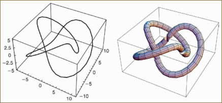
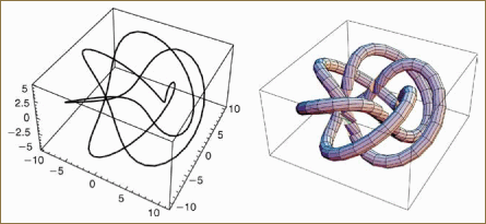
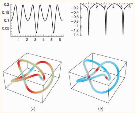
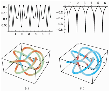
Examples of analytic curves: We begin with a classic mathematical example, the torus knot. The parametric equation of the (p, q) torus knot can be written as given in Equation 20.1. As examples of complex curve shapes, we choose a (2, 3) torus knot and a (3, 5) torus knot, and plot the 3D curves with and without an attached Frenet-frame tubing (Figures 20.8 and 20.9). We can learn some useful facts about the curve by computing its curvature and torsion. Following the work of Gray [31,61], we compute from Equations 20.15 and 20.16 the curvature and torsion for the (2, 3) and (3, 5) torus knots with size parameters (r, a, b) = (8, 3, 5), and use these quantities to choose values from an appropriate color table. The resulting values of the curvature and torsion are plotted and color encoded onto the curves themselves in Figures 20.10 and 20.11.
It is awkward to represent moving frames visually in high-density data because a frame consists of three 3D vectors (or nine components) yet has only three independent degrees of freedom. Some approaches to representing these degrees of freedom in a 3D space were suggested, for example, by Alpern et al. [3]. We propose instead to systematically exploit the representation of 3D orientation frames in four dimensions using equivalent unit quaternions that correspond, in turn, to points on the three-sphere (see, e.g., Shoemake [149]). For example, a collection of oriented frames such as those of a crystal lattice can thus be represented by mapping their orientations to a point set in the 4D quaternion space. The moving frame of a 3D space curve can be transformed into a path in quaternion space corresponding pointwise to the 3D space curve.
The quaternion representation of rotations reexpressing a moving frame of a 3D space curve is an elegant unit four-vector field over the curve. The resulting quaternion frames can be displayed as curves in their own right, or can be used in combination with other methods to enrich the display of each 3D curve (e.g., by assigning a coded display color representing a quaternion component).
Quaternions permit the nine matrix elements with six orthonormality constraints comprising a 3D orientation frame to be succinctly summarized in terms of four quaternion equations with the single constraint of unit length. Here we will derive the general features of these equations and how they are used to transform the standard 3D frame evolution equations into the more elegant quaternion form, which is essentially a square root of the conventional form.
We begin with a common formula for the correspondence between 3 × 3 matrices Rij and quaternions q :
[Recall that we use the notation * to distinguish quaternion multiplication, and will use the dot (·) when necessary to denote ordinary Euclidean inner products.] Next, we express each orthonormal frame component as a column of R by using an arbitrary quaternion to rotate each of the three Cartesian reference axes to a new, arbitrary orientation:
(Technically speaking, in Equation 20.18 ![]() really means the quaternion (0,
really means the quaternion (0, ![]() ) with only a vector part, and so on.) All of this can be transformed into the following explicit representation of the frame vectors as columns of a matrix of quaternion quadratic forms.
) with only a vector part, and so on.) All of this can be transformed into the following explicit representation of the frame vectors as columns of a matrix of quaternion quadratic forms.
Taking differentials of q*q–1 = (1,0), we generate expressions of the form
where
Substituting these expressions into the calculation for the first column, we find

The rest of the columns are computed similarly, and a straightforward expansion of the components of the cross products proves the correspondence between Equations 20.4 and 20.20.
To relate the derivative to a specific curve coordinate system, for example, we would introduce the curve velocity normalization v(t) = ‖x′(t)‖ and write
One of our favorite ways of rewriting this equation follows directly from the full form for the quaternion multiplication rule. Because this multiplication can be written as an orthogonal matrix multiplication on the 4D quaternion space, we could equally well write
This is the 3D analog of Equation 19.6.
Using Equation 20.24, we can express all 3D coordinate frames in the form of quaternions. If we assume that the columns of Equation 20.24 are the vectors (T, N, B), respectively, one can show from Equation 20.10 that [q′(t)] takes the form (see Hanson [68])
This equation has the following key properties.
The matrix on the right-hand side is antisymmetric, so that q(t) · q′(t) = 0 by construction. Thus, all unit quaternions remain unit quaternions as they evolve by this equation.
The number of equations has been reduced from nine coupled equations with six orthonormality constraints to four coupled equations incorporating a single constraint that keeps the solution vector confined to the three-sphere.
We verify that the matrices

explicitly reproduce Equation 20.10,

where we have applied Equation 20.25 to obtain the right-hand terms. Just as the Frenet equations may be integrated to generate a unique moving frame with its space curve for nonvanishing κ(t), we may integrate the much simpler quaternion Equations (20.25). (See Appendix H.)
Similarly, a parallel transport frame system given by Equation 20.13 with (N1, T, N2) (in that order) corresponding to the columns of Equation 20.24 is completely equivalent to the following parallel transport quaternion frame equation for [q′(t)].
Here, antisymmetry again guarantees that the quaternions remain constrained to the unit three-sphere. The correspondence to Equation 20.13 is verified as follows.

Given a particular curve, we are next faced with the task of assigning quaternion values to whatever moving frame sequence we have chosen.
The Frenet frame equations are pathological, for example, when the curve is perfectly straight for some distance or when the curvature vanishes momentarily. Thus, real numerical data for space curves will frequently exhibit behaviors that make the assignment of a smooth Frenet frame difficult, unstable, or impossible. In addition, because any given 3 × 3 orthogonal matrix corresponds to two quaternions that differ in sign, methods of deriving a quaternion from a Frenet frame are intrinsically ambiguous. Therefore, we prescribe the following procedure for assigning smooth quaternion Frenet frames to points on a space curve.
Select a numerical approach to computing the tangent T at a given curve point x. This typically depends on the chosen curve model and the number of points one wishes to sample.
Compute the remaining numerical derivatives at a given point and use those to compute the Frenet frame according to Equation 20.11. If any critical quantities vanish, tag the frame as undefined (or as needing a heuristic fix).
Check the dot product of the previous binormal B(t) with the current value. If it is near zero, choose a correction procedure to handle this singular point. Among the correction procedures we have considered are (1) simply jump discontinuously to the next frame to indicate the presence of a point with very small curvature, (2) create an interpolating set of points and perform a geodesic interpolation [149], or (3) deform the curve slightly before and after the singular point to “ease in” with a gradual rotation of the frame or apply an interpolation heuristic (e.g., see Shani and Ballard [147]). Creating a jump in the frame assignment is our default choice, since it does not introduce any new information.
Apply a suitable algorithm (e.g., see Chapter 16) to compute a candidate for the quaternion corresponding to the Frenet frame.
If the 3 × 3 Frenet frame is smoothly changing, make one last check on the 4D inner product of the quaternion frame with its own previous value. If there is a sign change, choose the opposite sign to keep the quaternion smoothly changing (this will have no effect on the corresponding 3 × 3 Frenet frame). If this inner product is near zero instead of ±1, you have detected a radical change in the Frenet frame that should have been noticed in the previous tests.
If the space curves of the data are too coarsely sampled to give the desired smoothness in the quaternion frames but are still close enough to give consistent qualitative behavior, one may choose to smooth out the intervening frames using the desired level of recursive SLERPing [145,149] to get smoothly splined intermediate quaternion frames. (More details can be found in Chapter 25.)
In Figure 20.12, we plot an example of a torus knot (a smooth space curve with everywhere nonzero curvature) together with its associated Frenet frames, its quaternion frame values, and the path of its quaternion frame field projected from four-space.

Figure 20.12. (a) Projected image of a 3D (3, 5) torus knot. (b) Selected Frenet frame components displayed along the knot. (c) The corresponding smooth quaternion frame components, with q0, q1 in the top row and q2, q3 in the bottom row. (d) The path of the quaternion frame components in the three-sphere projected from four-space. Color scales indicate the zeroth component of the curve’s four-vector frame (upper left-hand graph in c).
Figure 20.13 plots the same information, but this time for a curve with a discontinuous frame that flips instantly at a zero-curvature point. This space curve has two planar parts drawn as though on separate pages of a partly open book and meeting smoothly on the “crack” between pages. We see the obvious jump in the Frenet and quaternion frame graphs at the meeting point. If the two curves are joined by a long straight line, the Frenet frame is ambiguous and is essentially undefined in this segment. Rather than invent an interpolation, we generally prefer to use the parallel transport method described in the following section.

Figure 20.13. (a) Projected image of a pathological curve segment. (b) Selected Frenet frame components, showing a sudden change of the normal. (c) The quaternion frame components, with q0, q1 in the top row and q2, q3 in the bottom row, showing an unacceptable discontinuity in frame values. (d) The discontinuous path of the quaternion frame components in the three-sphere. Color scales indicate the zeroth component of the curve’s four-vector frame (upper left-hand graph in c).
To determine the quaternion frames of an individual curve using the parallel transport method, we follow a similar, but distinct, procedure.
Select a numerical approach to assigning a tangent at a given curve point as usual.
Assign an initial reference orientation to the initial point on the curve, in the plane perpendicular to the initial tangent direction. The entire set of frames will be displaced from the origin in quaternion space by the corresponding value of this initial orientation matrix, but the shape of the entire curve will be the same regardless of the initial choice. This choice is intrinsically ambiguous and application dependent. However, one appealing strategy is to base the initial frame on the first well-defined Frenet frame, and then proceed from there using the parallel transport frame evolution. This guarantees that identical curves have the same parallel transport frames.
Compute the angle between successive tangents, and rotate the frame by this angle in the plane of the two tangents to get the next frame value.
If the curve is straight, the algorithm automatically makes no changes.
Compute a candidate quaternion representation for the frame, applying consistency conditions (such as forcing positive signs of neighboring quaternion dot products) as needed.
Note that the initial reference orientation and all discrete rotations can be represented directly in terms of quaternions, and thus quaternion multiplication can be used directly to apply frame rotations. Local consistency is then automatic.
An example is provided in Figure 20.14, which shows the parallel transport analog of Figure 20.12 for a torus knot. Figure 20.15 is the parallel transport analog of the pathological case shown in Figure 20.13, but this time the frame is continuous when the curvature vanishes.

Figure 20.14. (a) Projected image of a 3D (3, 5) torus knot. (b) Selected parallel transport frame components displayed along knot. (c) The corresponding smooth quaternion frame components. (d) The path of the quaternion frame components in the three-sphere projected from four-space. Color scales indicate the zeroth component of the curve’s four-vector frame (upper left-hand graph in c).

Figure 20.15. (a) Projected image of a pathological curve segment. (b) Selected parallel transport frame components, showing smooth change of the normal. (c) The quaternion frame components, showing continuity in values. (d) The continuous path of the quaternion frame components in the three-sphere. Color scales indicate the zeroth component of the curve’s four-vector frame (upper left-hand graph in c).
The torus knot and the helix described previously (Equations 20.1 and 20.2) and shown in Figure 20.2 can now be studied in quaternion space using each of the representative frames. The comparison of each of our standard frames (Frenet, Bishop/parallel-transport, and geodesic reference) is depicted in Figure 20.16 for each of the curves.

Figure 20.16. Frenet (green), parallel transport (cyan), and geodesic reference (red) quaternion frames in “standard” 3D vector projection. (a) For the (2, 3) torus knot. (b) For the helix.
Labeled Red in Figure 20.16 is the geodesic reference framing. This is planar by construction, in that all 3D points must lie in the plane perpendicular to the reference axis. The 3D origin is at the centroid of the red curve. Labeled Green in the figure is the Frenet frame. The Frenet frame is actually cyclic, but to see this easily for this (2, 3) torus knot the mirror image of the current frame would need to be added, giving effectively a double traversal of the curve. Finally, we show the quaternion path (labeled Cyan) of the parallel transport frame. The parallel transport frame must be given a starting value, which here is chosen to coincide with the starting Frenet frame (at the top center of the image). The parallel transport frame is not cyclic, but is the shortest path, with three very noticeable tight loops. The same selection of quaternion frames is shown also for the helix. Again, the Red geodesic reference curve is planar (and cycles back on itself twice for this helix). The Green Frenet frame takes a longer path that will return to its original orientation, and the Cyan parallel transport frame, seen starting at the same orientation as the Frenet frame, will not ordinarily return to the same orientation but will have the shortest 4D path length. (The hidden double circuit of the geodesic reference frame for this helix in fact makes it longer.)
Previously (Figure 20.4) we compared the tubings for the (2, 3) torus knot and for the helix based on the Frenet, geodesic reference, and parallel transport frames. The corresponding quaternion paths are illustrated together in Figure 20.16. The parallel transport frame shown uses the initial Frenet frame as a starting point. We could, however, use any starting quaternion with the correct tangent vector. The relative path lengths of the curves shown in Figure 20.16 are summarized in Table 20.1. We note the following properties.
Table 20.1. Relative lengths (in radians) of the quaternion frame maps for various frame choices describing the (2, 3) torus knot and the helix. The parallel transport frame is the shortest possible frame map.
Curve Lengths | (2, 3) Torus Knot | Helix |
|---|---|---|
Frenet frame | 14.3168 | 6.18501 |
Geodesic reference frame | 14.6468 | 7.82897 |
Parallel transport frame | 10.1865 | 6.06301 |
Frenet: Periodic for periodic nonsingular curves and has a tendency to twist a bit too much (where the torsion is high), leaving long jumps between neighboring samples in quaternion space. Undefined at inflection points and zero curvature segments.
Geodesic reference: Also guaranteed to be periodic for periodic curves, but has the odd property that it always lies in a plane perpendicular to the reference axis in our preferred 3D quaternion projection. Ambiguous and therefore potentially not smooth for frames opposing the reference frame direction.
Parallel transport: This is the quaternion frame with minimal 4D length, though it may be difficult to see this feature immediately in our standard projection. It is not in general a periodic path. Different choices of starting frame produce curves of identical length differing by rigid 4D motions.
