Chapter 5. Applied Introduction to Machine Learning
Even though the forefront of artificial intelligence research captures headlines and our imaginations, do not let the esoteric reputation of machine learning distract from the full range of techniques with practical business applications. In fact, the power of machine learning has never been more accessible. Whereas some especially oblique problems require complex solutions, often, simpler methods can solve immediate business needs, and simultaneously offer additional advantages like faster training and scoring. Choosing the proper machine learning technique requires evaluating a series of tradeoffs like training and scoring latency, bias and variance, and in some cases accuracy versus complexity.
This chapter provides a broad introduction to applied machine learning with emphasis on resolving these tradeoffs with business objectives in mind. We present a conceptual overview of the theory underpinning machine learning. Later chapters will expand the discussion to include system design considerations and practical advice for implementing predictive analytics applications. Given the experimental nature of applied data science, the theme of flexibility will show up many times. In addition to the theoretical, computational, and mathematical features of machine learning techniques, the reality of running a business with limited resources, especially limited time, affects how you should choose and deploy strategies.
Before delving into the theory behind machine learning, we will discuss the problem it is meant to solve: enabling machines to make decisions informed by data, where the machine has “learned” to perform some task through exposure to training data. The main abstraction underpinning machine learning is the notion of a model, which is a program that takes an input data point and then outputs a prediction.
There are many types of machine learning models and each formulates predictions differently. This and subsequent chapters will focus primarily on two categories of techniques: supervised and unsupervised learning.
Supervised Learning
The distinguishing feature of supervised learning is that the training data is labeled. This means that, for every record in the training dataset, there are both features and a label. Features are the data representing observed measurements. Labels are either categories (in a classification model) or values in some continuous output space (in a regression model). Every record associates with some outcome.
For instance, a precipitation model might take features such as humidity, barometric pressure, and other meteorological information and then output a prediction about the probability of rain. A regression model might output a prediction or “score” representing estimated inches of rain. A classification model might output a prediction as “precipitation” or “no precipitation.” Figure 5-1 depicts the two stages of supervised learning.
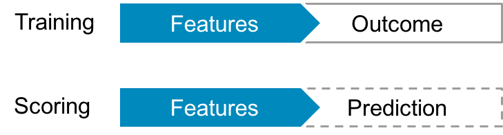
Figure 5-1. Training and scoring phases of supervised learning
“Supervised” refers to the fact that features in training data correspond to some observed outcome. Note that “supervised” does not refer to, and certainly does not guarantee, any degree of data quality. In supervised learning, as in any area of data science, discerning data quality—and separating signal from noise—is as critical as any other part of the process. By interpreting the results of a query or predictions from a model, you make assumptions about the quality of the data. Being aware of the assumptions you make is crucial to producing confidence in your conclusions.
Regression
Regression models are supervised learning models that output results as a value in a continuous prediction space (as opposed to a classification model, which has a discrete output space). The solution to a regression problem is the function that best approximates the relationship between features and outcomes, where “best” is measured according to an error function. The standard error measurement function is simply Euclidian distance—in short, how far apart are the predicted and actual outcomes?
Regression models will never perfectly fit real-world data. In fact, error measurements approaching zero usually points to overfitting, which means the model does not account for “noise” or variance in the data. Underfitting occurs when there is too much bias in the model, meaning flawed assumptions prevent the model from accurately learning relationships between features and outputs.
Figure 5-2 shows some examples of different forms of regression. The simplest type of regression is linear regression, in which the solution takes the form of the line, plane, or hyperplane (depending on the number of dimensions) that best fits the data (see Figure 5-3). Scoring with a linear regression model is computationally cheap because the prediction function in linear, so scoring is simply a matter of multiplying each feature by the “slope” in that direction and then adding an intercept.
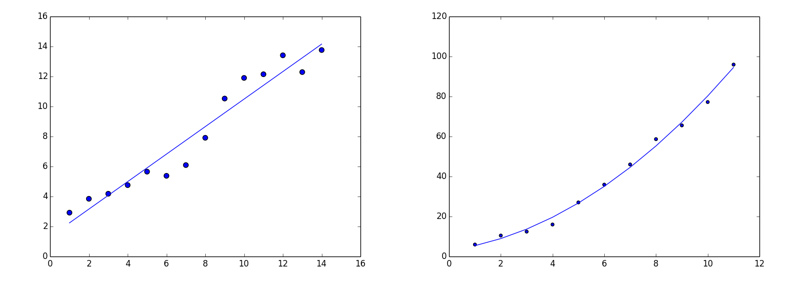
Figure 5-2. Examples of linear and polynomial regression
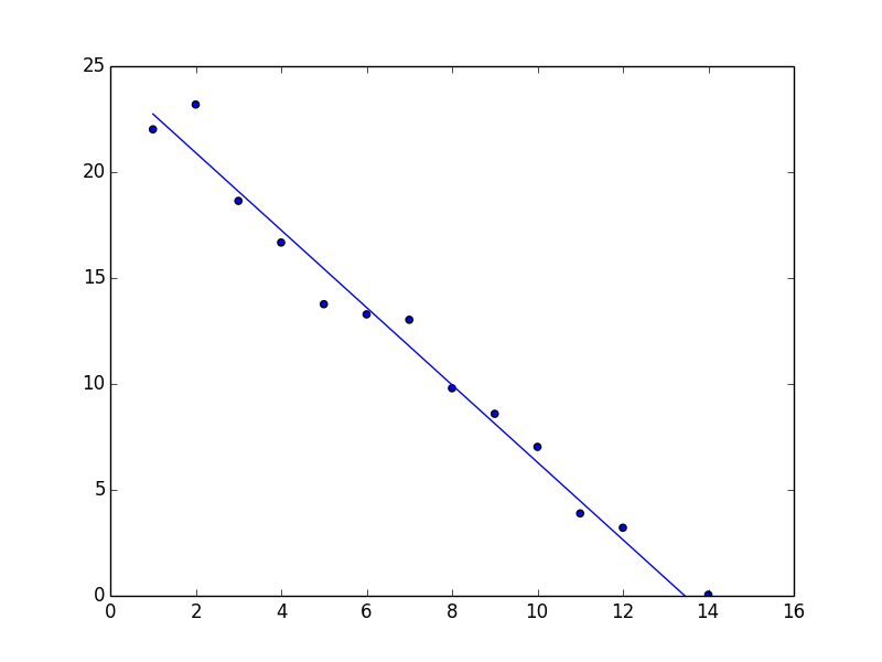
Figure 5-3. Linear regression in two dimensions
There are many types of regression and layers of categorization—this is true of many machine learning techniques. One way to categorize regression techniques is by the mathematical format of the solution. One form of solution is linear, where the prediction function takes the form of a line in two dimensions, and a plane or hyperplane in higher dimensions. Solutions in n dimensions take the following form:
a1x1 + a2x2 + … + an–1xn–1 + b
One advantage of linear models is the ease of scoring. Even in high dimensions—when there are several features—scoring consists of just scalar addition and multiplication. Other regression techniques give a solution as a polynomial or a logistic function. The following table describes the characteristics of different forms of regression.
| Regression model | Solution in two dimensions | Output space |
|---|---|---|
| Linear | ax + b | Continuous |
| Polynomial | a1xn + a2xn–1 + … + anx + an + an + 1 | Continuous |
| Logistic | L/(1 + e–k(x–x0)) | Continuous (e.g., population modeling) or discrete (binary categorical response) |
It is also useful to categorize regression techniques by how they measure error. The format of the solution—linear, polynomial, logistic—does not completely characterize the regression technique. In fact, different error measurement functions can result in different solutions, even if the solutions take the same form. For instance, you could compute multiple linear regressions with different error measurement functions. Each regression will yield a linear solution, but the solutions can have different slopes or intercepts depending on error function.
The method of least squares is the most common technique for measuring error. In least-squares approaches, you compute the total error as the sum of squares of the errors the solution relative to each record in the training data. The “best fit” is the function that minimizes the sum of squared errors. Figure 5-4 is a scatterplot and regression function, with red lines drawn in representing the prediction error for a given point. Recall that the error is the distance between the predicted outcome and the actual outcome. The solution with the “best fit” is the one that minimizes the sum of each error squared.
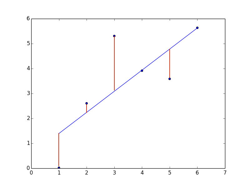
Figure 5-4. A linear regression, with red lines representing prediction error for a given training data point
Least squares is commonly associated with linear regression. In particular, a technique called Ordinary Least Squares is a common way of finding the regression solution with the best fit. However, least-squares techniques can be used with polynomial regression, as well. Whether the regression solution is linear or a higher degree polynomial, least squares is simply a method of measuring error. The format of the solution, linear or polynomial, determines what shape you are trying to fit to the data. However, in either case, the problem is still finding the prediction function that minimizes error over the training dataset.
Although Ordinary Least Squares provides a strong intuition for what the error measurement function represents, there are many ways of defining error in a regression problem. There are many variants on least-squares error function, such as weighted least squares, in which some observations are given more or less weight according to some metric that assesses data quality. There are also various approaches that fall under regularization, which is a family of techniques used to make solutions more generalizable rather than overfit to a particular training set. Popular techniques for regularized least squares includes Ridge Regression and LASSO.
Whether you’re using the method of least squares or any other technique for quantifying error, there are two sources of error: bias, flawed assumptions in model that conceal relationships between the features and outcomes of a dataset, and variance, which is naturally occurring “noise” in a dataset. Too much bias in the model causes underfitting, whereas too much variance causes overfitting. Bias and variance tend to inversely correlate—when one goes up the other goes down—which is why data scientists talk about a “bias-variance tradeoff.” Well-fit models find a balance between the two sources of error.
Classification
Classification is very similar to regression and uses many of the same underlying techniques. The main difference is the format of the prediction. The intuition for regression is that you’re matching a line/plane/surface to approximate some trend in a dataset, and every combination of features corresponds to some point on that surface. Formulating a prediction is a matter of looking at the score at a given point. Binary classification is similar, except instead of predicting by using a point on the surface, it predicts one of two categories based on where the point resides relative to the surface (above or below). Figure 5-5 shows a simple example of a linear binary classifier.
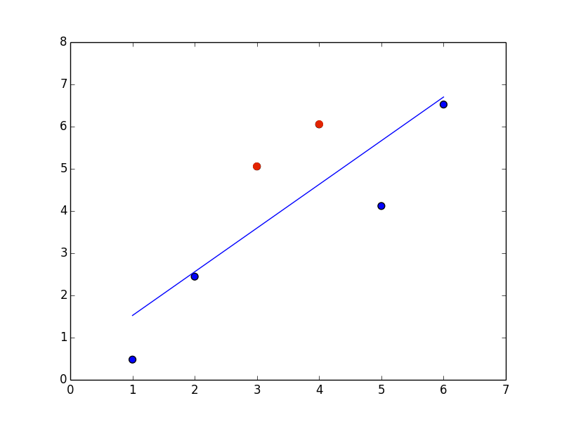
Figure 5-5. Linear binary classifier
Binary classification is the most commonly used and best-understood type of classifier, in large part because of its relationship with regression. There are many techniques and algorithms that are used for training both regression and classification models.
There are also “multiclass” classifiers, which can use more than two categories. A classic example of a multiclass classifier is a handwriting recognition program, which must analyze every character and then classify what letter, number, or symbol it represents.
Unsupervised Learning
The distinguishing feature of unsupervised learning is that data is unlabeled. This means that there are no outcomes, scores, or categorizations associated with features in training data. As with supervised learning, “unsupervised” does not refer to data quality. As in any area of data science, training data for unsupervised learning will not be perfect, and separating signal from noise is a crucial component of training a model.
The purpose of unsupervised learning is to discern patterns in data that are not known beforehand. One of its most significant applications is in analyzing clusters of data. What the clusters represent, or even the number of clusters, is often not known in advance of building the model. This is the fundamental difference between unsupervised and supervised learning, and why unsupervised learning is often associated with data mining—many of the applications for unsupervised learning are exploratory.
It is easy to confuse concepts in supervised and unsupervised learning. In particular, cluster analysis in unsupervised learning and classification in supervised learning might seem like similar concepts. The difference is in the framing of the problem and information you have when training a model. When posing a classification problem, you know the categories in advance and features in the training data are labeled with their associated categories. When posing a clustering problem, the data is unlabeled and you do not even know the categories before training the model.
The fundamental differences in approach actually create opportunities to use unsupervised and supervised learning methods together to attack business problems. For example, suppose that you have a set of historical online shopping data and you want to formulate a series of marketing campaigns for different types of shoppers. Furthermore, you want a model that can classify a wider audience, including potential customers with no purchase history.
This is a problem that requires a multistep solution. First you need to explore an unlabeled dataset. Every shopper is different and, although you might be able to recognize some patterns, it is probably not obvious how you want to segment your customers for inclusion in different marketing campaigns. In this case, you might apply an unsupervised clustering algorithm to find cohorts of products purchased together. Using this clustering information to your purchase data then allows you to build a supervised classification model that correlates purchasing cohort with other demographic information, allowing you to classify your marketing audience members without a purchase history. Using an unsupervised learning model to label data in order to build a supervised classification model is an example of semi-supervised learning.
Cluster Analysis
Cluster analysis programs detect patterns in the grouping of data. There are many approaches to clustering problems, but each has some measure of “closeness” and then optimizes arrangements of clusters to minimize the distance between points within a cluster.
Perhaps the easiest method of cluster analysis to grasp are centroid-based techniques like k-means. Centroid-based means that clusters are defined so as to minimize distances from a central point. The central point does not need to be a record in the training data—it can be any point in the training space. Figure 5-6 includes two scatterplots, the second of which includes three centroids (k = 3).
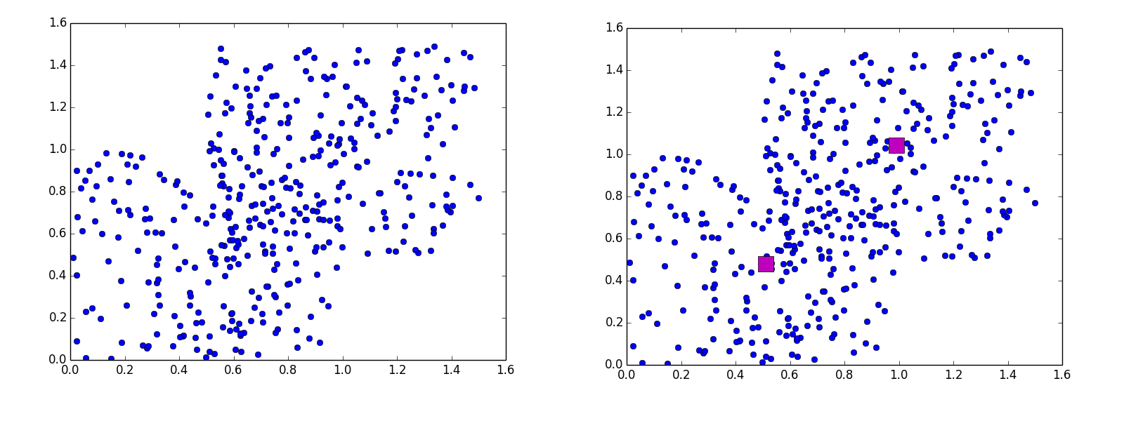
Figure 5-6. Sample clustering data with centroids determined by k-means
The “k” in k-means refers to the number of centroids. K-means algorithms iterate through values of k and choose optimal placements for the k centroids at each iteration so as to minimize the mean distance from training data points to centroid for each cluster. Figure 5-7 shows two examples of k-means applied to the same dataset but with different values of k.
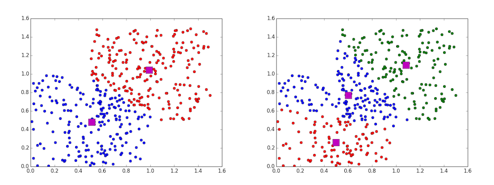
Figure 5-7. K-means examples with k = 2 and k = 3, respectively
There are many other methods for cluster analysis. Hierarchical methods derive sequences of increasingly large and inclusive clusters, as clusters combine with other nearby clusters at different stages of the model. These methods produce trees of clusters. On one end of the tree is a single node: one cluster that includes every point in the training. At the other end, every data point is its own cluster. Neither extreme is useful for analysis, but in between there is an entire series of options for dividing up the data into clusters. The method chooses an optimal depth in the hierarchy of clustering options.
Anomaly Detection
Although anomaly detection is its own area of study, one approach follows naturally from the discussion of clustering. Algorithms for clustering methods iterate through series of potential groupings; for example, k-means implementations iterate through values of k and assess them for fit. Because there is noise in any real world dataset, models that are not overfitted will leave outliers that are not part of any cluster.
Another class of methods (that still bears resemblance to cluster analysis) looks for local outliers that are unusually far away from their closest neighbors.