Renewable Energy and Industrial IoT

The market around the Industrial Internet of Things (IIoT) is rapidly expanding, and is set to reach $150 billion in 2020, according to research firm Markets and Markets. According to the firm,

IIoT is the integration of complex physical machinery with industrial networks and data analytics solutions to improve operational efficiency and reduce costs.

Renewable energy is an equally high growth sector. In mid-2016, Germany announced that it had developed almost all of its power from renewable energy (“Germany Just Got Almost All of Its Power From Renewable Energy,” May 15, 2016).

The overall global growth in renewable energy continues at a breakneck pace, with the investment in renewables reaching $286 billion worldwide in 2015 (BBC).

PowerStream: A Showcase Application of Predictive Analytics for Renewable Energy and IIoT

PowerStream is an application that predicts the global health of wind turbines. It tracks the status of nearly 200,000 wind turbines around the world across approximately 20,000 wind farms. With each wind turbine reporting multiple sensor updates per second, the entire workload ranges between 1 to 2 million inserts per second.

The goal of the showcase is to understand the sensor readings and predict the health of the turbines. The technical crux is the volume of data as well as its continuous, dynamic flow. The underlying data pipeline needs to be able to capture and process this in real-time.

PowerStream Hardware Configuration

With the power of distributed systems, you can implement rich functionality on a small consolidated hardware footprint. For example, the PowerStream architecture supports high-volume real-time data pipelines across the following:

• A message queue

• A transformation and scoring engine, Spark

• A stateful, persistent, memory-optimized database

• A graphing and visualization layer

The entire pipeline runs on just seven cloud server instances, in this case Amazon Web Services (AWS) C-2x large. At roughly $0.31 per hour per machine, the annual hardware total is approximately $19,000 for AWS instances.

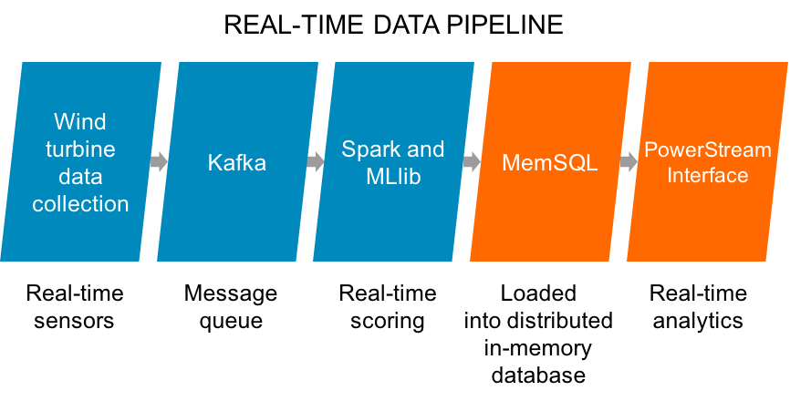
Figure 8-1. PowerStream software architecture

The capability to handle such a massive task with such a small hardware footprint is a testament to the advances in distributed and memory-optimized systems.

PowerStream Application Introduction

The basics of the interface include a visualization layer. The windfarm and turbine colors represent state based on data sent from the turbines to Kafka, then through Streamliner for machine learning with Spark, then on to MemSQL. This stream begins with integers and tuples (doubles?) emitted from each turbine.

After data is in a memory-optimized database, you can take interesting approaches such as building applications on that live, streaming data. In PowerStream, we use a developer-friendly mapping tool called Mapbox which provides a mapping layer embedded in a browser. Mapbox has an API and enables rapid development of dynamic applications.

For example, zooming in to the map (see Figure 8-2) allows for inspection from the windfarm down to the turbine level, and even seeing values of individual sensors.

One critical juncture of this application is the connection between Spark and the database, enabled by the MemSQL Spark Connector. The performance and low latency comes from both systems being distributed and memory optimized, so working with Resilient Distributed Datasets and Dataframes becomes very efficient as each node in one cluster communicates with each node in another cluster. This speed makes building an application easier. The time from ingest, to real-time scoring, and then being saved to a relational database can easily be less than one second. At that point, any SQL-capable application is ready to go.

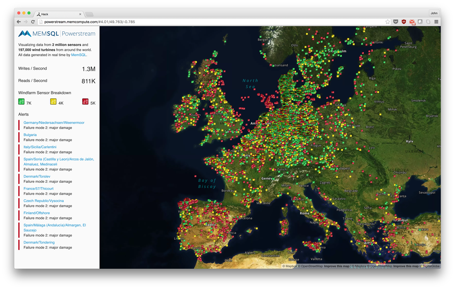
Figure 8-2. PowerStream application introduction

Adding the machine learning component delivers a rich set of applications and alerts with many types of sophisticated logic flowing in real time.

For example, we classify types of potential failures by predicting which turbines are failing and, more specifically, how they are failing. Understandably, the expense of a high-cost turbine not working is significant. Predictive alerts enable energy utilities to deploy workforces and spare parts efficiently.

Because data in a relational, SQL-capable database is extremely accessible to most enterprises, a rich set of Business Intelligence (BI) tools experience the immediate benefit of real-time data. For example, the screenshots presented in Figure 8-3 and Figure 8-4 show what is possible with Tableau.

And when failures are introduced into the system, the dashboard changes to a mix of yellow and red.

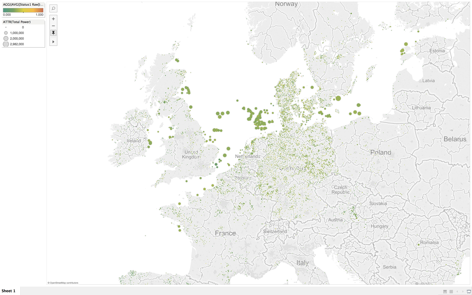
Figure 8-3. PowerStream interface using Tableau—status: healthy

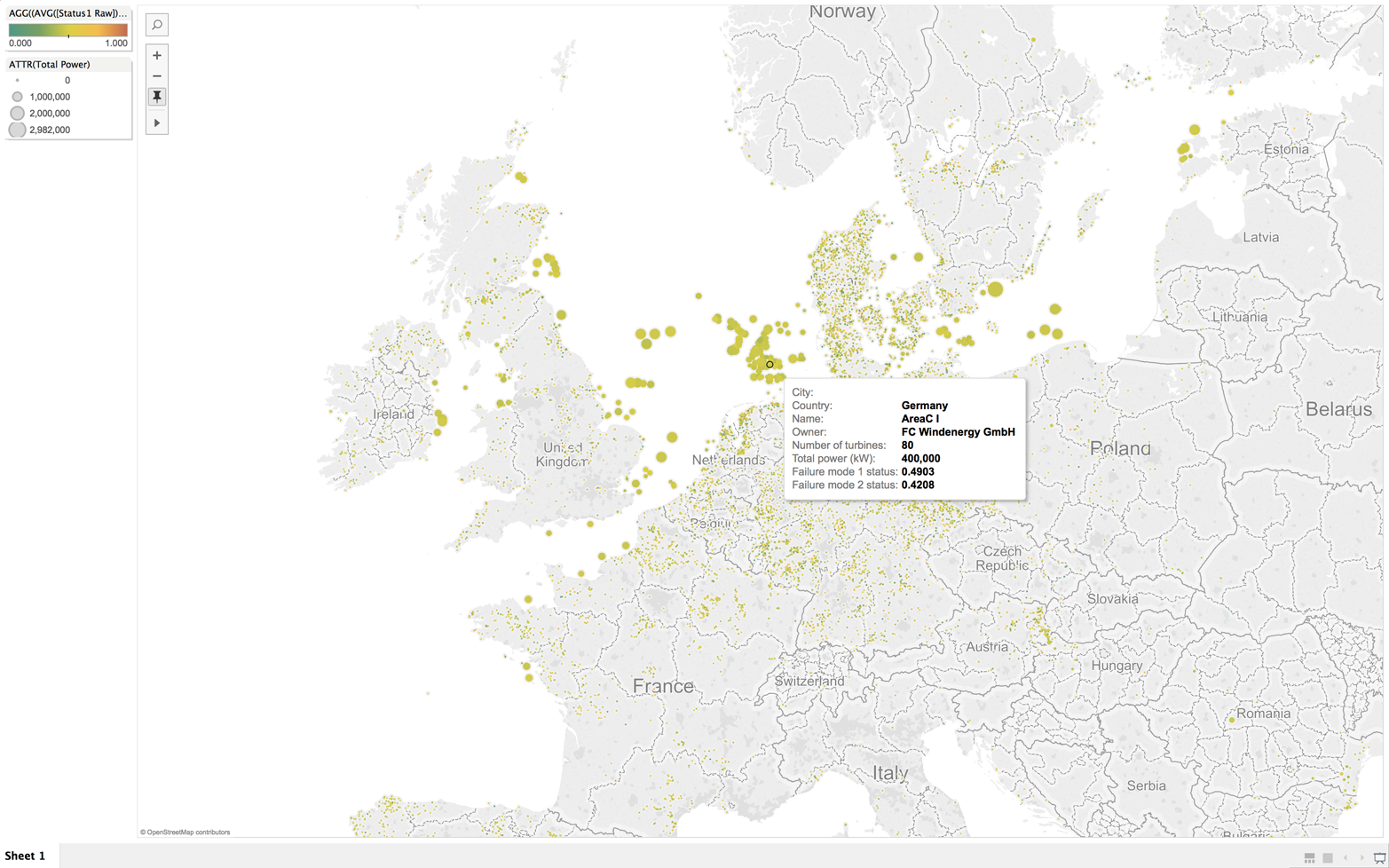
Figure 8-4. PowerStream interface using Tableau—status: warnings

PowerStream Details

One layer down in the application, updates come from simulated sensor values. Turbine locations are accurate based on a global database, with concentrations in countries like Germany, which is known for renewable energy success.

PowerStream sets a column in the turbine table to a value. Based on that value, the application can predict if the turbine is about to fail. Yellow or red indicates different failure states.

Examining the specific pipelines, we see one for scoring called ML and one for alerts (see Figure 8-5).

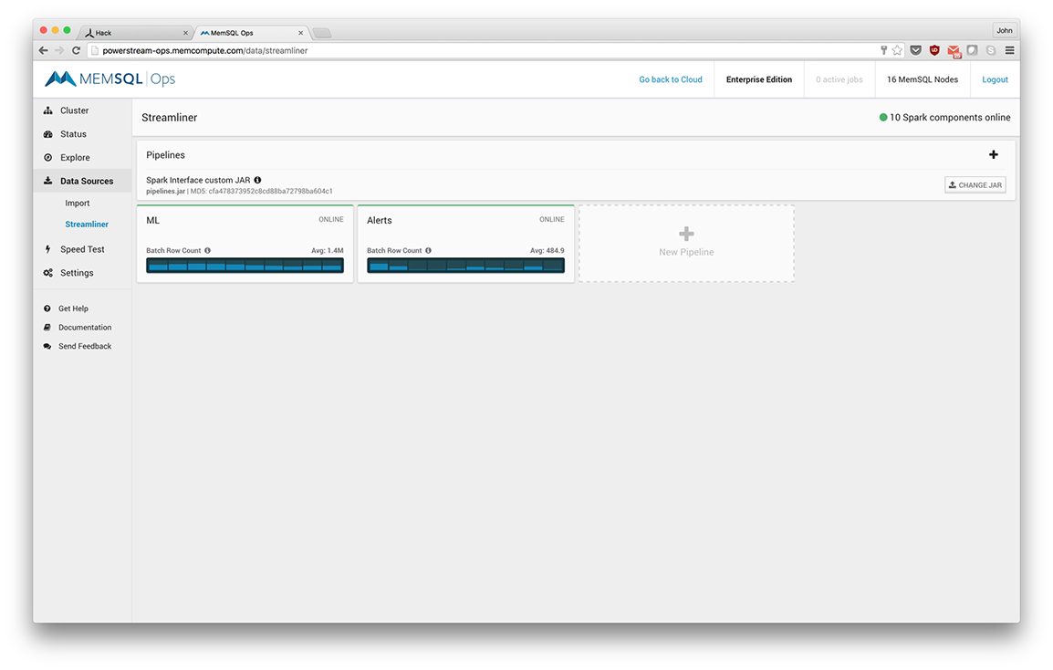
Figure 8-5. ML and Alerts pipelines

The ML pipeline shows throughput in the 1 to 2–million-transaction-per-second range (see Figure 8-6).

Figure 8-6. The ML pipeline showing throughput in the 1 to 2 million transactions-per-second range

The Alerts pipeline shows throughput in the 500-rows-per-second range (see Figure 8-7).

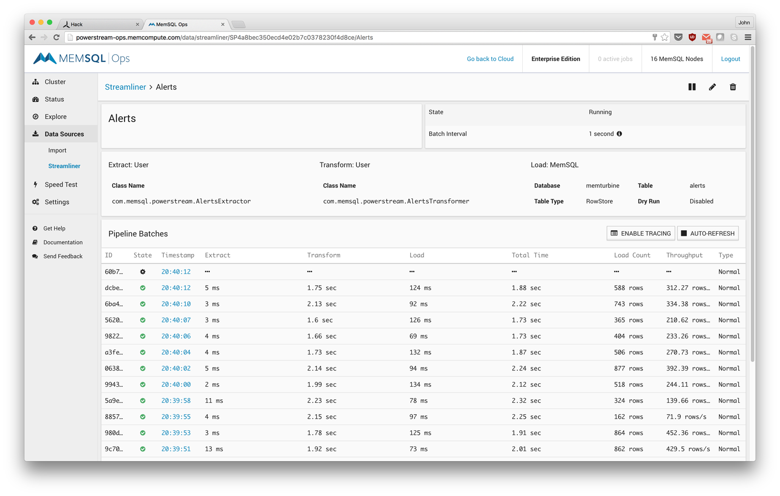
Figure 8-7. The Alerts pipeline showing throughput in the 500-rows-per-second range

The data from Kafka comes by simply identifying the Zookeeper quorum IP address for the Kafka cluster.

Within the Streamliner application, you can create a transform in Scala or Python. If you’re using Python, you can edit the transformation within the browser. If you’re using Scala, you determine the Class and you can change the JAR file that has the definition of that class.

Implementation is straightforward as Streamliner and Spark apply the machine learning model for each record coming in from Kafka and pushed into the database, under the table name Sensors.

One advantage of storing the pipeline in a database is the ability to store data efficiently. In this pipeline, on duplicate key behavior, data is replaced. More specifically, every data point updates a value for a particular wind turbine and instead of just accumulating this data, we update it.

SQL Pushdown Details

Unlike a job-scheduled system like Spark, an in-memory database like MemSQL is continually operating in real time, and requests are processed live. There are no jobs created, and there is no job management. This architecture responds at the millisecond level and delivers great concurrency.

This low latency and high concurrency support for SQL compliments Spark capabilities, and provides a persistent, transactional storage layer. The overarching use case is Spark as a high-level interface, with key functions such as persistence, accelerated query execution, and concurrency pushed down to the in-memory database.

PowerStream at the Command Line

To examine the power of Spark and MemSQL together, we can jump into the Spark shell and take a look at a query and its definition.

In the example that follows, we are selecting a turbine ID with two subselects joining on a complex condition. This is not an equality join but rather a join on distance, whether the status of one row is within a particular distance from another side of the join.

scala> query
res11: String =
"
SELECT a.turbine_id
FROM
    (SELECT * FROM turbines_model WHERE windfarm_id < 100) a,
    (SELECT * FROM turbines_model WHERE windfarm_id < 100) b
WHERE
    abs(a.status1_raw - b.status1_raw) < 0.00000000001
"

If we look at the explain plan, we see how Spark would run the query. One operator of particular note is CartesianProduct, which likely has a lengthy impact on query execution.

scala> val dfNoPushdown = mscNoPushdown.sql(query)
dfNoPushdown: org.apache.spark.sql.DataFrame = [turbine_id: int]

scala> dfNoPushdown.explain()
== Physical Plan ==
TungstenProject [turbine_id#16]
 Filter (abs((status1_raw#17 - status1_raw#24)) < 1.0E-11)
  CartesianProduct
   ConvertToSafe
    TungstenProject [turbine_id#16,status1_raw#17]
     Filter (windfarm_id#15L < 100)
      Scan MemSQLTableRelation(MemSQLCluster(MemSQLConf
      (10.0.1.140,3306,root,KPVyNu98Kv8CjRcm,memturbine,
        ErrorIfExists,DatabaseAndTable,10000,GZip)),
          `memturbine`.`turbines_model_out`,
            com.memsql.spark.connector.MemSQLContext@4402630e)
              [windfarm_id#15L,turbine_id#16,status1_raw#17,
                status1#18L,status2_raw#19,
                  status2#20L,status#21L]
   ConvertToSafe
    TungstenProject [status1_raw#24]
     Filter (windfarm_id#22L < 100)
      Scan MemSQLTableRelation(MemSQLCluster(MemSQLConf
      (10.0.1.140,3306,root,KPVyNu98Kv8CjRcm,memturbine,
        ErrorIfExists,
        DatabaseAndTable,10000,GZip)),
          `memturbine`.`turbines_model_out`,
          com.memsql.spark.connector.MemSQLContext@4402630e)
            [windfarm_id#22L,turbine_id#23,
              status1_raw#24,status1#25L,
              status2_raw#26,status2#27L,status#28L]

If we enable SQL pushdown, we can see at the top the MemSQL RDD, which pushes the query execution directly into the database.

scala> val df = msc.sql(query)
df: org.apache.spark.sql.DataFrame = [turbine_id: int]

scala> df.explain()
== Physical Plan ==
MemSQLPhysicalRDD[SELECT (`f_7`) AS `turbine_id` FROM (SELECT  
(`query_1`.`f_4`) AS `f_7` FROM 
(SELECT (`query_1_1`.`f_1`) AS `f_4`, 
(`query_1_1`.`f_2`) AS `f_5`, (`query_2_1`.`f_3`) AS `f_6` FROM 
(SELECT (`query_1_2`.`turbine_id`) AS `f_1`, 
(`query_1_2`.`status1_raw`) AS `f_2` FROM (SELECT * FROM 
(SELECT * FROM `memturbine`.`turbines_model_out`) AS `query_1_3`  
  WHERE (`query_1_3`.`windfarm_id` < ?)) AS `query_1_2`) 
    AS `query_1_1` INNER JOIN (SELECT  
    (`query_2_2`.`status1_raw`) AS `f_3` FROM (SELECT * FROM 
    (SELECT * FROM `memturbine`.`turbines_model_out`) 
      AS `query_2_3`  WHERE 
      (`query_2_3`.`windfarm_id` < ?)) AS `query_2_2`) 
        AS `query_2_1` WHERE  
        (ABS((`query_1_1`.`f_2` - `query_2_1`.`f_3`)) < ?)) 
          AS `query_1`) AS `query_0`]
  PartialQuery[query_0, f_7#45] ((`query_1`.`f_4`) AS `f_7`) ()
    JoinQuery[query_1, f_4#45,f_5#46,f_6#53] 
    ((`query_1_1`.`f_1`) AS `f_4`, (`query_1_1`.`f_2`) AS `f_5`, 
    (`query_2_1`.`f_3`) AS `f_6`) ((ABS
    ((`query_1_1`.`f_2` - `query_2_1`.`f_3`)) < ?))
      PartialQuery[query_1_1, f_1#45,f_2#46] 
      ((`query_1_2`.`turbine_id`) AS `f_1`, 
      (`query_1_2`.`status1_raw`) AS `f_2`) ()
        PartialQuery[query_1_2, windfarm_id#44L,turbine_id#45,
          status1_raw#46,status1#47L,status2_raw#48,status2#49L,
            status#50L] () ( WHERE 
            (`query_1_3`.`windfarm_id` < ?))
          BaseQuery[query_1_3, windfarm_id#44L,turbine_id#45,
            status1_raw#46,status1#47L,status2_raw#48,
              status2#49L,status#50L] 
              (SELECT * FROM `memturbine`.`turbines_model_out`)
      PartialQuery[query_2_1, f_3#53] 
      ((`query_2_2`.`status1_raw`) AS `f_3`) ()
        PartialQuery[query_2_2, windfarm_id#51L,turbine_id#52,
          status1_raw#53,status1#54L,status2_raw#55,
            status2#56L,status#57L] () ( WHERE 
            (`query_2_3`.`windfarm_id` < ?))
          BaseQuery[query_2_3, windfarm_id#51L,turbine_id#52,
            status1_raw#53,status1#54L,
              status2_raw#55,status2#56L,status#57L] 
              (SELECT * FROM `memturbine`.`turbines_model_out`)
()

scala> df.count()
res7: Long = 1615

scala> df.count()
res8: Long = 1427

scala> df.count()
res9: Long = 1385

scala> df.count()
res10: Long = 1565

With this type of query, a SQL-optimized database like MemSQL can achieve a response in two to three seconds. With Spark, it can take upward of 30 minutes. This is due to the investment made in a SQL-optimized engine and executing sophisticated queries that utilize the query optimizer and query execution facilities of MemSQL. Databases also make use of indexes, which keep query latency low.

Of course, you also can access MemSQL directly. Here, we are taking the same query from the preceding example and showing the explain plan in MemSQL:

EXPLAIN SELECT a.turbine_id
    FROM
        (SELECT 
            * 
        FROM 
            turbines_model_out 
        WHERE 
            windfarm_id < 100) a,
        (SELECT 
            * 
        FROM 
            turbines_model_out 
        WHERE 
            windfarm_id < 100) b
    WHERE
        abs(a.status1_raw - b.status1_raw) < 0.00000000001;
+--------------------------------------------------------------+
| EXPLAIN                                                                                                                                  |
+--------------------------------------------------------------+
| Project [a.turbine_id]                                                                                                                   |
| Filter [ABS(a.status1_raw - b.status1_raw) < .00000000001]                                                                               
| NestedLoopJoin                                                                                                                           |
| |---TableScan 1tmp AS b storage:list stream:no                                                                                           
| |   TempTable                                                                                                                            |
| |   Gather partitions:all                                                                                                                |
| |   Project [turbines_model_out_1.status1_raw]                                                                                           |
| |   IndexRangeScan memturbine.turbines_model_out AS 
  turbines_model_out_1, PRIMARY KEY 
  (windfarm_id, turbine_id) scan:[windfarm_id < 100] |
| TableScan 0tmp AS a storage:list stream:yes                                                                                              
| TempTable                                                                                                                                |
| Gather partitions:all                                                                                                                    |
| Project [turbines_model_out.turbine_id,    
  turbines_model_out.status1_raw]                                                                  
| IndexRangeScan memturbine.turbines_model_out, PRIMARY KEY 
  (windfarm_id, turbine_id) scan:[windfarm_id < 100]                             
+--------------------------------------------------------------+

This is a distributed plan that begins with an index scan and a nested loop. Applying the predicate windfarm_id < 100 enables the database to take advantage of that index.

This query runs in parallel. There is a Gather operator to pull the data into the aggregator.

We do a similar operation for other side of join, and within that perform a nested loop join.

For every record on one table, we are looking up that record in another table according to the predicate of the condition of that join.

Using the power of Kafka, Spark, and an in-memory database like MemSQL together, you can go from live data to predictive analytics in a few simple steps. This quickly gets the technology into the business to be more efficient with critical assets.