C H A P T E R  10

Infrastructure and Operations

Creating fast and scalable software is, of course, central to building an ultra-fast web site. However, the design of your production hardware and network environment, the process of deploying your software into production, and the process you follow to keep everything running smoothly are also vitally important factors.

Most web sites are evolving entities; their performance and character change over time as you add and remove code and pages, as your traffic increases, and as the amount of data that you are managing increases. Even if your end-to-end system is fast to begin with, it may not stay that way unless you plan ahead.

Establishing the right hardware infrastructure and being able to deploy new releases quickly and to detect and respond to performance problems quickly are key aspects of the ultra-fast approach.

In this chapter, I will cover the following:

• Instrumentation
• Capacity planning
• Disk subsystems
• Network design
• Firewalls and routers
• Load balancers
• DNS
• Staging environments
• Deployment
• Server monitoring

Instrumentation

I have seen many web sites that look fast during development but rapidly slow down when they get to production. A common scenario is a site that runs well most of the time but suffers from occasional dramatic slowdowns. Without the proper infrastructure and operations process, debugging performance and scalability problems can be extremely challenging and time-consuming. One tool that can be immensely helpful is instrumentation in the form of Windows performance counters (or just counters for short).

Counters are lightweight objects that you can use to record not only counts of various events (as the name implies) but also timing-related information. You can track averages as well as current values. Counters are integrated with Windows. You can view them using perfmon. You can see them as a graph or chart in real time, or you can record them into a file for later processing. You can also see them from a remote machine, given the appropriate permissions. Even for an application that is very rich in counters, the incremental CPU overhead is well under 1 percent.

All of Microsoft’s server products include custom counters. Your applications should use them for the same reason Microsoft does: to aid performance tuning, to help diagnose problems, and to help identify issues before they become problems.

Here are some guidelines on the kinds of things that you should consider counting or measuring with counters:

• All off-box requests, such as web service calls and database calls, both in general (total number of calls) and specifically (such as the number of site login calls).
• The time required to generate certain web pages.
• The number of pages processed, based on type, category, and so on. The built-in ASP.NET and IIS counters provide top-level, per-web-site numbers.
• Queue lengths (such as for background worker threads).
• The number of handled and unhandled exceptions.
• The number of times an operation exceeds a performance threshold.

For the last point, the idea is to establish performance thresholds for certain tasks, such as database calls. You can determine the thresholds based on testing or dynamic statistics. Your code then measures how long those operations actually take, compares the measurements against the thresholds, and increments a counter if the threshold is exceeded. Your goal is to establish an early warning system that alerts you if your site’s performance starts to degrade unexpectedly.

You can also set counters conditionally, based on things such as a particular username, browser type, and so on. If one user contacts you and reports that the site is slow, but most people say it’s OK, then having some appropriate counters in place can provide a way for you get a breakdown of exactly which parts of that user’s requests are having performance problems.

There are several types of counters:

• NumberOfItems32
• NumberOfItems64
• NumberOfItemsHEX32
• NumberOfItemsHEX64
• RateOfCountsPerSecond32
• RateOfCountsPerSecond64
• CountPerTimeInterval32
• CountPerTimeInterval64
• RawFraction
• RawBase
• AverageTimer32
• AverageBase
• AverageCount64
• SampleFraction
• SampleCounter
• SampleBase
• CounterTimer
• CounterTimerInverse
• Timer100Ns
• Timer100NsInverse
• ElapsedTime
• CounterMultiTimer
• CounterMultiTimerInverse
• CounterMultiTimer100Ns
• CounterMultiTimer100NsInverse
• CounterMultiBase
• CounterDelta32
• CounterDelta64

Counters are organized into named categories. You can have one category for each major area of your application, with a number of counters in each category.

Here’s an example of creating several counters in a single category (see Program.cs):

You create a new 32-bit integer counter called Logins and a 64-bit average counter called Ave Users, along with its base counter, in a new category called Membership. Base counters must always immediately follow average counters. The reported value is the first counter divided by the base.

To create new counters programmatically or to read system counters, your application needs either to have administrative privileges or to be a member of the Performance Monitor Users group. For web applications, you should add your AppPool to that group, to avoid having to run with elevated privileges. You can do that by running the following command:

If you’re using the default identity for IIS 7.5 (ApplicationPoolIdentity), then replace DefaultAppPool with the name of your AppPool. Otherwise, use the identity’s fully qualified name, such as NT AUTHORITYNETWORK SERVICE.

Alternatively, you can use the Computer Management GUI to do the same thing.

1. Open Local Users and Groups and click on Groups.
2. Double-click on Performance Monitor Users.
3. Click Add, enter IIS AppPoolDefaultAppPool and click on Check Names to confirm. Finally, click OK.

You can also create counters on your local machine from Server Explorer in Visual Studio. Expand Servers, click your machine name, right-click Performance Counters, and select Create New Category. See Figure 10-1.

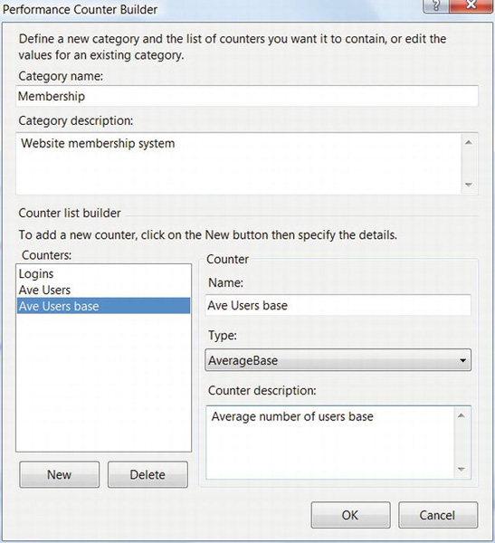
Figure 10-1. Adding new performance counters from Server Explorer in Visual Studio

Using a counter is even easier than creating one:

You increment the value in the Logins counter you created previously. You can also IncrementBy() an integer value or set the counter to a specific RawValue.

Counters can be either single instance or multi-instance, as in the example. A single instance counter has the same value everywhere you reference it on your machine. For example, the total CPU use on your machine would be a single instance counter. You use multi-instance counters when you want to track several values of the same type. In the example above, you might have several applications that you want to track separately. For multi-instance counters, you specify the instance name when you create the counter, and you can select which instances you want to view when you run perfmon.

After your web site is running and you have created your counters, you can select and view them using perfmon, as you did in Chapter 8 for SQL Server. The description you used when you created the counter is visible at the bottom of the window when you select the Show description checkbox. See Figure 10-2.

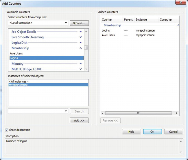
Figure 10-2. Selecting custom performance counters with perfmon

Once your application is running and you’ve selected the counters that you’re interested in, perfmon can show them either as a graph or in report form, as in Figure 10-3.

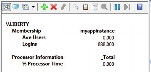
Figure 10-3. Viewing performance counters in the report format

Capacity Planning

As your site grows, if you wish to avoid unexpected surprises with regard to performance, it’s important to be able to anticipate the future performance of your site under load. You should be able to track the current load on your servers over time and use that information to predict when you will need additional capacity.

During development, you should place a maximum load on your servers and observe how they behave. As you read earlier, if you’re using synchronous threads, it may not be possible to bring your servers anywhere close to 100 percent CPU use. Even so, whatever that limit is on your system, you should understand it. Another argument for using async threads is that they allow increased CPU use, so they improve both overall hardware utilization and capacity planning.

Next, it’s important to minimize the different types of servers you deploy in your web tier. If you have one type of server to handle membership, another for profiles, another for content, and so on, then each one will behave differently under load. One type of server may reach its capacity, while the others are close to idle. As your site grows, it becomes increasingly difficult to predict which servers will reach their capacity before others. In addition, it’s generally more cost effective to allow multiple applications to share the same hardware. That way, heavily loaded applications can distribute their load among a larger number of servers. That arrangement also smoothes the load on all the servers and makes it easier to do capacity planning by forecasting the future load based on current load.

If necessary, you can use WSRM to help balance the load among different AppPools or to provide priority to some over others, as discussed in Chapter 4.

You should track performance at all the tiers in your system: network, web, data, disk, and so on. The CPU on your database server may be lightly loaded, while its disk subsystem becomes a bottleneck. You can track that by collecting a standard set of counters regularly when your system is under load. You can use perfmon, or you can write an application that reads the counters and publishes them for later analysis.

Disk Subsystems

Disks are mechanical devices. They contain rotating magnetic media and heads that move back and forth across that media, where they eventually read or write your data. See Figure 10-4.

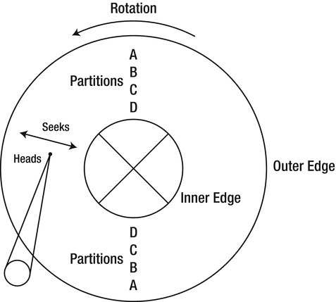
Figure 10-4. Physical disk platter and heads

Most modern drives support Native Command Queuing (NCQ), which can queue multiple requests and service them in an order that is potentially different from the order in which you submitted them. The drives also use RAM to buffer data from reads and can sometimes be used to buffer write data. Data on the media is organized into physical 512-byte blocks, which is the minimum size that the drive can read or write at a time.

Random vs. Sequential I/Os per Second

One way to measure disk performance is in terms of the number of reads and/or writes (I/Os) per second (IOPS) at a given buffer size.

As an example, consider a typical 15,000rpm SAS disk. At that speed, it takes 4ms for the media to complete one rotation. That means to go from one random rotational position to another takes, on average, half that time, or 2ms. Let’s say the average time for the heads to move (average seek) is 2.9ms for reads and that the average time to read 8KB (SQL Server’s page size) is 0.12ms. That makes the total 5.02ms. Over one second, the drive can make about 199 of those 8KB random reads, or 199IOPS. That’s only 1.6MB/sec. In other words, when disks operate in random mode, they can be extremely slow.

If the disk is reading sequentially, then the average maximum sustainable read rate may be about 70MBps. That’s 8,750IOPS, or 44 times faster than random mode. With such a large difference, clearly anything you can do to encourage sequential access is very important for performance.

This aspect of disk performance is why it’s so important to place database log files on a volume of their own. Because writes to the log file are sequential, they can take advantage of the high throughput the disks have in that mode. If the log files are on the same volume as your data files, then the writes can become random, and performance declines accordingly.

One cause of random disk accesses is using different parts of the same volume at the same time. If the disk heads have to move back and forth between two or more areas of the disk, performance can collapse compared to what it would be if the accesses were sequential or mostly sequential. For that reason, if your application needs to access large files on a local disk, it can be a good idea to manage those accesses through a single thread.

This issue often shows up when you copy files. If you copy files from one place to another on the same volume without using a large buffer size, the copy progresses at a fraction of the rate that it can if you copy from one physical spindle to another. The cost of introducing extra disk seeks is also why multithreaded copies from the same disk can be so slow.

NTFS Fragmentation

The NTFS filesystem stores files as collections of contiguous disk blocks called clusters. The default cluster size is 4KB, although you can change it when you first create a filesystem. The cluster size is the smallest size unit that the operating system allocates when it grows a file. As you create, grow, and delete files, the space that NTFS allocates for them can become fragmented; it is no longer contiguous. To access the clusters in a fragmented file, the disk heads have to move. The more fragments a file has, the more the heads move, and the slower the file access.

One way to limit file fragmentation is to run a defragmentation utility regularly. If your servers tend not to be busy at a particular time of the day or week, you can schedule defragmentation during those times. However, if you require consistent 24 × 7 performance, then it’s often better to take one or a few servers offline while defragmentation is running because the process can completely saturate your disk subsystem.

To schedule regular disk defragmentation, right-click the drive name in Windows Explorer, and select Properties. Click the Tools tab, and then click Defragment Now, as shown in Figure 10-5.

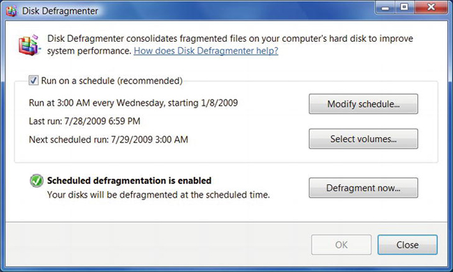
Figure 10-5. Scheduling periodic disk defragmentation

If your system regularly creates and deletes a large number of files at the web tier, then periodic defragmentation can play an important role in helping to maintain the performance of your system.

You may also encounter cases where you have a few specific files that regularly become fragmented. In that case, instead of defragmenting your entire drive, you may want to defragment just those files. Alternatively, you may want to check to see how many fragments certain files have. For both of those scenarios, you can use the contig utility. It’s available as a free download:

http://technet.microsoft.com/en-us/sysinternals/bb897428.aspx

For example, you can use contig as follows to see how many fragments a file has:

You defragment the file like this:

When you create a large file on a new and empty filesystem, it will be contiguous. Because of that, to ensure that your database data and log files are contiguous, you can put them on an empty, freshly created filesystem and set their size at or near the maximum they will need. You also shouldn’t shrink the files because they can become fragmented if they grow again after shrinking.

If you need to regularly create and delete files in a filesystem and your files average more than 4KB in size, you can minimize fragmentation by choosing an NTFS cluster size larger than that. Although the NTFS cluster size doesn’t matter for volumes that contain only one file, if your application requires mixing regular files with database data or log files, you should consider using a 64KB NTFS cluster size to match the size of SQL Server extents.

Before your application begins to write a file to disk, you can help the operating system minimize fragmentation by calling FileStream.SetLength() with the total size of the file. Doing so provides the OS with a hint that allows it to minimize the number of fragments it uses to hold the file. If you don’t know the size of the file when you begin writing it, you can extend it in 64KB or 128KB increments as you go (equal to one or two SQL Server extents) and then set it back to the final size when you’re done.

You can help maximize the performance of NTFS by limiting how many files you place in a single folder. Although disk space is the only NTFS-imposed limit on the number of files you can put in one folder, I’ve found that limiting each folder to no more than about 1,000 files helps maintain optimal performance. If your application needs significantly more files than that, you can partition them into several different folders. You can organize the folders by something like the first part of file name to help simplify your partitioning logic.

Disk Partition Design

You can improve the throughput of your disks by taking advantage of the fact that the outer edge of the disk media moves at a faster linear speed than the inner edge. That means that the maximum sustainable data transfer rate is higher at the outer edge.

Figure 10-6 shows example transfer rates for a 15,000rpm 73GB SAS drive. The left side of the chart shows the transfer rate at the outer edge, and the right side is the inner edge.

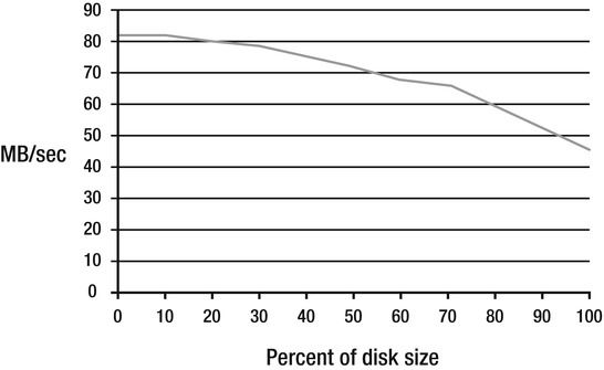
Figure 10-6. Sustained disk transfer rates based on the location of the data on the disk

You can see that the maximum transfer rate only holds over about the first 30 percent of the drive. After that, performance declines steadily. At the inner edge of the drive, the maximum transfer rate is only about 55 percent of the rate at the outer edge.

In addition, you can reduce average seek times by placing your data only in a narrow section of the disk. The narrower the area, the less distance the heads have to travel on average.

For random access, minimizing seek times is much more important than higher data rates. For sequential access, the reverse is true.

Extending the previous example, let’s say you have a 73GB drive. You can make a partition covering the first 30 percent of the drive, which is about 20GB. The first partitions you create on a drive are at the outer edge of the media, as shown in Figure 10-4. The rotational latency in that partition is still 2ms, but the average seek is reduced from 2.9ms to about 1.2ms. (Seek times aren’t linear; the heads accelerate when they start and then decelerate as they approach the destination.) The data-transfer time is a tiny bit better, dropping from 0.12ms to 0.10ms. The total is 3.3ms, which is about 303IOPS. That’s about a 50 percent improvement in random disk I/O throughput, simply by limiting the size of the partition. You can improve throughput even more by further reducing the partition’s size.

For an equal partition size, you can increase disk performance further by using drives with more platters because doing so lets you use physically narrower partitions for the same amount of space. The drives electronically switch between different heads to access the additional platters. That switching time doesn’t affect latency; so, for example, the average seek for the example 20GB partition may drop to around 0.44ms, which increases throughput to about 394IOPS, or roughly twice the original value.

Of course, that’s still a far cry from sequential throughput. The next step in increasing disk performance is to use several disks together as a RAID volume.

RAID Options

The most common types of RAID are 0, 1, 5, and 10. RAID 3 and 6 are less common but are still useful in certain environments. In my experience, the others are rarely used.

RAID 0 and Stripe Size

RAID 0, also known as disk striping, puts one small chunk of data on one drive, the next logical chunk on the next drive, and so on. It doesn’t use any redundancy, so if one drive in a volume fails, the rest of the data in the volume is also lost. As such, it is not an appropriate configuration to use in production.

The size of the chunk of data on each drive is sometimes known as the strip size. The strip size times the number of drives is the stripe size. If your application reads that many bytes at once, all of the drives are active at the same time.

Let’s say you have four drives configured as a RAID 0 volume. With a 64KB stripe size, the strip size is 16KB. If you read 16KB from the beginning of the volume, only the first drive is active. If you read 32KB, the first two drives are active at the same time. With 64KB, the controller requests 16KB from all four drives at once. With individual 16KB requests, your I/O throughput is still limited to the speed of a single drive. With 64KB per read, it is four times as high. What you see in practice is somewhere in between, with the details depending not only on your application but also on the particular disk controller hardware you’re using. There is quite a bit of variability from one vendor to another in terms of how efficiently controllers are able to distribute disk I/O requests among multiple drives, as well as how they handle things like read-ahead and caching.

RAID 1

RAID 1 is also known as mirroring. The controller manages two disks so that they contain exactly the same data. The advantage compared to RAID 0 is that if one of the drives fails, your data is still available. Read throughput can in theory be faster than with a single drive because the controller can send requests to both drives at the same.

RAID 5

RAID 5 extends RAID 0 by adding block-level parity data to each stripe. The location of the parity data changes from one drive to the next for each stripe. Unlike with RAID 0, if one of the drives fails, your data is safe because the controller can reconstruct it from the remaining data and the parity information. Reads can be as almost as fast as with RAID 0 because the controller doesn’t need to read the parity unless there’s a failure. Writes that are less than a full stripe size need to read the old parity first, then compute the new parity, and write it back. Because the controller writes the new parity to the same physical location on the disk as the old parity, the controller has to wait a full rotation time before the parity write completes. A battery-backed cache on the controller can help.

If the controller receives a write request for the full stripe size on a RAID 5 volume, it can write the parity block without having to read it first. In that case, the performance impact is minimal.

When you stripe several RAID 5 volumes together, it’s known as RAID 50.

RAID 10

RAID 10 is a combination of RAID 1 and RAID 0. It uses mirroring instead of parity, so it performs better with small block writes.

RAID 3

RAID 3 is like RAID 5, except it uses byte-level instead of block-level parity, and the parity data is written on a single drive instead of being distributed among all drives. RAID 3 is slow for random or multithreaded reads or writes, but can be faster than RAID 5 for sequential I/O.

RAID 6

RAID 6 is like RAID 5, except that instead of one parity block per stripe, it uses two. Unfortunately, as disk drive sizes have increased, unrecoverable bit error rates haven’t kept pace, at about 1 in 10¹⁴ bits (that’s 10TB) for consumer drives, up to about 1 in 10¹⁶ bits for Enterprise drives. With arrays that are 10TB or larger, it begins to be not just possible but likely that, in the event of a single drive failure, you can also have an unrecoverable error on a second drive during the process of recovering the array. Some controllers help reduce the probability of a double-failure by periodically reading the entire array. RAID 6 can help mitigate the risk even further by maintaining a second copy of the parity data.

RAID 5 with a hot spare is a common alternative to RAID 6. Which approach is best depends heavily on the implementation of the controller and its supporting software.

RAID Recommendations

Although the exact results differ considerably by controller vendor, Table 10-1 shows how the most common RAID technologies roughly compare to one another, assuming the same number of drives for each.

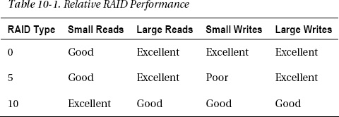
I didn’t include RAID 1 because you can consider it to be a two-drive RAID 10. Keep in mind as well that although I’ve included RAID 0 for comparative purposes, it isn’t suitable for production environments because it doesn’t have any redundancy.

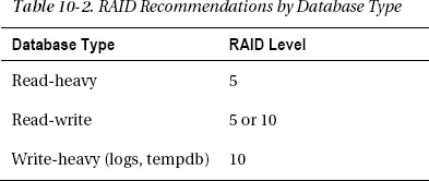
Although SQL Server’s disk-access patterns vary, as a rule of thumb for data files, it tends to read 64KB extents (large reads) and write 8KB pages (small writes). Because RAID 5 does poorly with small writes and very well for large reads, it’s a good choice for databases that either are read-only or are not written very much. Either RAID 5 or 10 can work well for databases with typical read/write access patterns, depending on the details of your system, including both hardware and software. RAID 10 is usually the best option for the write-heavy database log and tempdb. See Table 10-2.

If you’re using RAID 5, depending on your specific controller hardware, a stripe size of 64KB is a good place to start, so that it’s the same as the SQL Server extent size. That should enable better performance for large writes. For RAID 10, the stripe size isn’t as important. In theory, a smaller stripe size should be more efficient. Unfortunately, in practice, it doesn’t seem to work out that way because of controller quirks. Even so, if you have enough drives that you can spread out a stripe so that one 8KB SQL Server page is split between at least two drives, that should help.

Although the technology is always evolving, I’ve found that SAS or SCSI drives work best in high-performance arrays. One reason is that their implementations of NCQ seem to be more effective when compared to those in SATA drives. NCQ can help minimize latency as the disk-queue depth increases. It works by sorting the requests in the queue by their proximity to the current location of the disk heads, using an elevator algorithm. The heads move in one direction until there are no more requests to service, before reversing and moving in the other direction. SAS drives support bidirectional communication with the drive, which is helpful during heavy use. They also tend to have better MTBF and bit error rates than SATA drives.

When you are designing high-performance disk arrays, you should apply the same partitioning strategy that you used for the single-drive case: one small, high-speed partition at the beginning of the array for your data. You can follow that with a second smaller partition to hold tempdb, a third small partition for the system databases (master, model, and msdb), and a fourth for backups, which occupies most of the volume.

You should also consider controller throughput. A PCIe 2.0 x8 controller should be capable of roughly 2.0GBps of throughput. At 400IOPS per drive, a single drive can read only 3.2MBps in random access mode, or around 75MBps in sequential mode. On an OLTP system, where the workload is a mix of random and sequential, you can estimate that total throughput might peak at around 25MBps per drive. That means a maximum of about 80 drives per controller for the data files and up to about 13 drive pairs (26 drives) per controller for log files and other sequential access.

As your system grows, you can put a new SQL Server filegroup on each new volume.

The requirements for data warehouse staging or reporting databases are somewhat different. Because the tables are usually larger and because you should design the system to handle table and index scans as it exports data to SSAS, more of the I/O is sequential, so the sustainable maximum I/O rate is higher. You may want only half as many drives per controller compared to the OLTP case. I would expect the disk-queue length to be substantially higher on a staging database under load than on an OLTP system.

Storage Array Networks

An alternative to piecing together a customized disk subsystem is to use a storage array network (SAN). SANs are great for environments where reliability is more important than performance, or where you prefer to rely on an outside vendor to help set up, tune, and configure your disk subsystem, or in heavily shared environments. It can be very handy to be able to delegate that work to an outside firm so that you have someone to call if things break. The disadvantage is cost.

Using the information I’ve presented here, you can readily build an array that outperforms a SAN in most scenarios for a fraction of the price. However, in many shops, do-it-yourself configurations are discouraged, and that’s where SANs come in.

You should be cautious about two things with SANs. First, you shouldn’t consider a huge RAM cache or other tiered storage in the SAN to be a cure-all for performance issues. It can sometimes mask them for a while, but the maximum sustained performance is ultimately determined by the drives, not by how much cache the system has. Second, when it comes to SQL Server in particular, recall from the earlier discussion about how it manages memory so that it becomes a huge cache. Provided SQL Server has enough RAM, that makes it difficult for a SAN to cache something useful that SQL Server hasn’t already cached.

Another issue is focusing only on random IOPS. I’ve seen some SANs that don’t allow you to differentiate between random and sequential IOPS when you configure them. One solution, in that case, is to put a few extra drives in the CPU chassis and to use those for your log files instead of the SAN.

Controller Cache

The issue with cache memory also applies to controllers. The cache on controllers can be helpful for short-duration issues such as rotational latency during RAID 5 writes. However, having a huge cache can be counterproductive. I encourage you to performance-test your system with the disk controller cache disabled. I’ve done this myself and have found multiple cases where the system performs better with the cache turned off.

The reasons vary from one controller to another, but in some cases, disabling the cache also disables controller read-ahead. Because SQL Server does its own read-ahead, when the controller tries to do it too, it can become competitive rather than complementary.

Solid State Disks

Solid state disks (SSDs) built with flash memory are starting to become price-competitive with rotating magnetic media on a per-GB basis, when you take into account that the fastest part of conventional disks is the first 25 to 30 percent.

SSDs have huge performance and power advantages over disks because they don’t have any moving parts. Rotational delay and seek times are eliminated, so the performance impact is extremely significant. Random access can be very fast, and issues such as fragmentation are not as much of a concern from a performance perspective.

Flash-based SSDs have some unique characteristics compared to rotating magnetic media:

• They use two different underlying device technologies: multilevel cell (MLC) and single-level cell (SLC) NAND memory.
• You can only write them between roughly 10,000 (MLC) and 100,000 (SLC) times before they wear out (even so, they should last more than 5 years in normal use).
• Write speeds with SLC are more than twice as fast as MLC.
• SLC has nearly twice the mean time between failure (MTBF) of MLC (typically 1.2M hours for MLC and 2.0M hours for SLC).
• MLC-based devices have about twice the bit density of SLC.

SSDs are organized internally as a mini-RAID array, with multiple channels that access multiple arrays of NAND memory cells in parallel. The memory consists of sectors that are grouped into pages. The details vary by manufacturer, but an example is 4KB sectors and 64KB pages.

With disks, you can read and write individual 512-byte sectors. With SSDs, you can read an individual sector, but you can only write at the page level and only when the page is empty. If a page already contains data, the controller has to erase it before it can be written again.

SSDs have sophisticated vendor-specific controllers that transparently manage the page-erase process. The controllers also vary the mapping of logical to physical block addresses to help even out the wear on the memory cells (wear leveling).

Typical performance of a single SSD for sequential reads is close to the limit of the SATA 3.0 Gbps interface specification, at 250MBps. Typical sequential write speeds for an MLC device are 70MBps, with SLC at around 150MBps.

SSDs with SATA interfaces are compatible with standard RAID controllers. By grouping several SSDs in RAID, you can easily reach the limit of PCIe bus bandwidth for sequential reads on a single volume, although you are likely to hit the controller’s limit first. PCIe 2.0 throughput is about 600MBps per channel, or 4.8GBps for an x8 slot; a good x8 controller can deliver close to 2.0GBps.

SSDs have already started to augment and replace rotating magnetic drives in high-performance production environments. I expect that trend to continue.

Disk Array Benchmarks

Table 10-3 shows some benchmark results for a few disk arrays.

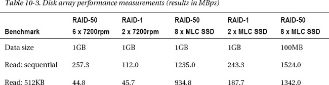
The disk controller I used for all of the benchmarks except the SSD RAID-1 was an LSI Logic 9260-8i with 512MB cache and the FastPath option. The SSD RAID-1 controller was an ICH-10 on the motherboard. I configured the arrays with a 32KB strip size, and enabled write-back caching for the RAID-50 SSDs, with a battery backup on the controller card. The 7200rpm drives have a 1TB capacity each, and were configured with write-through caching.

I ran all of the benchmarks except one with a 1GB file size, which is large enough that it doesn’t fit in the controller’s cache. The final test was with a 100MB file size, which does fit in cache, so it’s more a demonstration of the controller’s performance than the underlying drive’s performance.

I used a benchmark program called CrystalDiskMark. The tests are sequential access, random with 512KB blocks and QD=1 (queue depth), random 4KB blocks QD=1, and random 4KB blocks QD=32. Queue depth is a measure of how many requests are outstanding at the same time. I generally use the 512KB results as a first cut when estimating SQL Server’s OLTP performance.

A few observations about the results:

• The SSD two-drive RAID-1 mirror has as much sequential read performance as the 7200rpm 6-drive RAID-50 array, and more than four times the 512KB read performance.
• The SSD eight-drive RAID-50 array is nearly five times as fast for sequential reads as the 7200rpm 6-drive RAID-50 array, nearly 21 times as fast for 512KB reads, and more than 30 times as fast for 4KB reads.
• The 7200rpm two-drive RAID-1 mirror is faster than the six-drive RAID-50 array for all write benchmarks except with high queue depth because the controller needs to read the parity information on the RAID-50 array before writing it.
• Sequential writes are 22 times faster when the active volume’s working set fits in the controller’s cache in write-back mode because the software doesn’t have to wait for the write to be committed to the media before it can indicate success.

Network Design

One source of latency in your data center is the network that connects your servers. For example, a 100Mbps network has an effective data-transfer rate of up to roughly 10MBps. That means a 100KB response from your database takes 10ms to transfer, and 100 such requests per second will saturate the link.

Recall from the earlier discussion of threading in ASP.NET that long request latency can have a significant adverse impact on the scalability of your site and that the issue is compounded if you are making synchronous requests. If you were to increase the speed of the network connection to 1Gbps, with effective throughput of roughly 100MBps, that would reduce the latency for a 100KB response from 10ms to just 1ms, or 1,000 requests per second.

The issue isn’t performance; reducing the time that it takes to process a single request by 9ms won’t visibly improve the time it takes to load a page. The issue is scalability. A limited number of worker threads are available at the web tier. In synchronous mode, if they are all waiting for data from the data tier, then any additional requests that arrive during that time are queued. Even in async mode, a limited number of requests can be outstanding at the same time; and the longer each request takes, the fewer total requests per second each server can process.

The importance of minimizing latency means that network speeds higher than 1Gbps are generally worthwhile when scalability is a concern. 10Gbps networking hardware is starting to be widely available, and I recommend using it if you can.

For similar reasons, it’s a good idea to put your front-end network on one port and your back-end data network on a separate port, as shown later in Figure 10-8. Most commercial servers have at least two network ports, and partitioning your network in that way helps to minimize latency.

Jumbo Frames

Another way to increase throughput and reduce latency on the network that connects your web servers to your database is to enable jumbo frames. The maximum size of a standard Ethernet packet, called the maximum transmission unit (MTU), is 1,518 bytes. Most gigabit interfaces, drivers, and switches (although not all) support the ability to increase the maximum packet size to as much as 9,000 bytes. Maximum packet sizes larger than the standard 1,518 bytes are called jumbo frames. They are available only at gigabit speeds or higher; they aren’t available on slower 100Mbps networks.

Each packet your servers send or receive has a certain amount of fixed overhead. By increasing the packet size, you reduce the number of packets required for a given conversation. That, in turn, reduces interrupts and other overhead. The result is usually a reduction in CPU use, an increase in achievable throughput, and a reduction in latency.

An important caveat with jumbo frames is that not only do the servers involved need to support them, but so does all intermediate hardware. That includes routers, switches, load balancers, firewalls, and so on. Because of that, you should not enable jumbo frames for ports or interfaces that also pass traffic to the Internet. If you do, either the server has to take time to negotiate a smaller MTU, or the larger packets are fragmented into smaller ones, which has an adverse impact on performance. Jumbo frames are most useful on your physically private network segments, such as the ones that should connect your web and database servers.

To enable jumbo frames, follow these steps:

1. On Windows Server, start Server Manager, select Diagnostics in the left panel, and then choose Device Manager. On Windows 7, right-click on Computer, select Manage, and then choose Device Manager in the left-hand panel.
2. Under Network Adapters in the center panel, right-click on a gigabit interface, and select Properties.
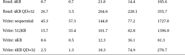
3. Click the Advanced tab, select Jumbo Frame (the string is vendor-specific, so it might be something similar like Jumbo MTU or Jumbo Packet), and set the MTU size, as shown in Figure 10-7.

Repeat the process for all machines that will communicate with each other, setting them all to the same MTU size.

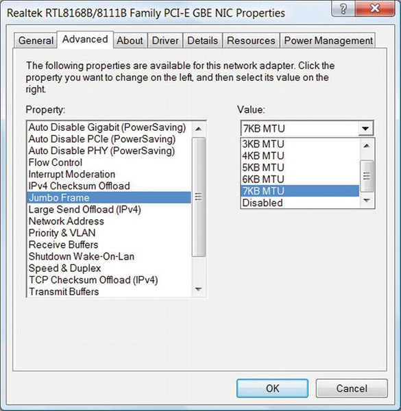
Figure 10-7. Enabling jumbo frames on your network interface

Link Aggregation

If you have more than one web server, then another technique for increasing throughput and decreasing latency for your database servers is to group two network ports together so they act as a single link. The technology is called link aggregation and is also known as port trunking or NIC teaming. It is managed using the Link Aggregation Control Protocol (LACP), which is part of IEEE specification 802.3ad. Unfortunately, this isn’t yet a standard feature in Windows, so the instructions on how to enable it vary from one network interface manufacturer to another. You need to enable it both on your server and on the switch or router to which the server is connected.

After you enable it, link aggregation lets your server send and receive data at twice the rate it would be able to otherwise. Particularly in cases where multiple web servers are sharing a single database, this can help increase overall throughput. See Figure 10-8.

If you have only one web server, you should have one network port for connections to the Internet and one for the database. Link aggregation won’t help in that case, unless your web server happens to have three network ports instead of the usual two.

Figure 10-8. Optimized network design with jumbo frames and link aggregation

Firewalls and Routers

When you are considering whether a server-side firewall would be appropriate for your environment, it’s important to take your full security threat assessment into account. The biggest threats that most web sites face are from application vulnerabilities such as SQL injection or cross-site scripting, rather than from the kinds of things that firewalls protect against.

From a performance and scalability perspective, you should be aware that a firewall might introduce additional latency and other bottlenecks, such as limiting the number of simultaneous connections from browsers to web servers.

It’s my view that most vanilla web sites don’t need hardware firewalls. These firewalls can be a wonderful tool for protecting against things such as downloading malicious files or accidentally introducing a virus by connecting an unprotected laptop to your network. However, in a production environment, you should prohibit arbitrary downloads onto production servers and connecting client-type hardware to the production network, which dramatically reduces the risk of introducing viruses or other malware. A large fraction of the remaining types of external attacks can be prevented by simply filtering out all requests for connections to ports other than 80 (HTTP) or 443 (SSL).

Another service that hardware firewalls can provide is protection against network transport layer attacks, such as denial of service. If those are a concern for you, and if you don’t have access to your router, then a hardware firewall may be worth considering.

If you do use a hardware firewall, you should place it between your router and your load balancer, as shown in Figure 10-7, so that it can filter all traffic for your site.

Another valid use for hardware firewalls is as a virtual private network (VPN) endpoint. You should not have a direct path from the public Internet to your back-end database servers. To bypass port filtering and to gain access to those back-end servers, you should connect to your remote servers over VPN. Ideally, the VPN should connect to a separate management network, so the VPN endpoint doesn’t have to handle the full traffic load of your site.

Windows Firewall and Antivirus Software

You can apply port-filtering functions using Windows Firewall, which you should enable on all production servers. Using a software firewall also helps protect you against a variety of threats that hardware firewalls can’t address, such as application bugs that may allow an attacker to connect from one server to another. Because those attacks don’t normally go through the hardware firewall on their way from one server to another, they can’t be filtered that way, whereas a software firewall running on each machine can catch and filter that type of network traffic.

On smaller sites, where your users can upload files onto your servers, you should consider using server-side antivirus software as an alternative to a hardware firewall.

Using Your Router as an Alternative to a Hardware Firewall

In most hosted environments, you don’t need a router of your own; your ISP provides it for you. However, as your site grows, at some point you will want to take over management of your network connection, including having a router. Having access to your router also means you can use it to help improve the performance and security of your site. For example, you can use it to do port filtering. Many routers, including those that run Cisco IOS, also support protection against things like SYN floods and other denial-of-service attacks. Being able to offload that type of work onto your router, and thereby avoid the need for a hardware firewall, can help minimize latency while also reducing hardware and ongoing maintenance costs.

Load Balancers

As your site grows and as resilience in the event of hardware failures becomes more important, you will need to use some form of load balancing to distribute incoming HTTP requests among your servers. Although a hardware solution is certainly possible, another option is network load balancing (NLB), which is a standard feature with Windows Server.

NLB works by having all incoming network traffic for your virtual IP addresses (normally, those are the ones public users connect to) delivered to all your servers and then filtering that traffic in software. It does therefore consume CPU cycles on your servers. The scalability tests I’ve seen show that NLB can be a reasonable option up to no more than about eight servers. Beyond that, the server-to-server overhead is excessive, and hardware is a better choice.

As with hardware load balancers, keep in mind that NLB works at the link protocol level, so you can use it with any TCP- or UDP-based application, not just IIS or HTTP. For example, you can use it to load-balance DNS servers.

To configure NLB, follow these steps:

1. Install the Network Load Balancing feature from Server Manager.
2. Open the Network Load Balancing Manager from Administrative Tools.
3. Right-click Network Load Balancing Clusters in the left pane, select New Cluster, and walk through the wizard.

When you are selecting load balancing hardware, pay particular attention to network latency. As with the other infrastructure components, minimizing latency is important for scalability.

In addition to its usual use in front of web servers, another application for load balancing is to support certain configurations in the data tier. For example, you may distribute the load over two or more identical read-only database servers using NLB.

You can also use reverse load balancing (RLB) to facilitate calls from one type of web server to another from within your production environment, such as for web services. As with public-facing load balancing, RLB lets you distribute the internal load among multiple servers and to compensate in the event of a server failure.

DNS

Before a client’s browser can talk to your web site for the first time, it must use DNS to resolve your hostname into an IP address. If your site uses a number of subdomains, as I suggested in Chapter 2, then the client’s browser needs to look up each of those addresses. The time it takes for name resolution has a direct impact on how quickly that first page loads.

DNS data is cached in many places: in the browser, in the client operating system, in the user’s modem or router, and in their ISP’s DNS server. Eventually, though, in spite of all the caches, your DNS server must deliver the authoritative results for the client’s query.

There’s a whole art and science to making DNS fast and efficient, particularly in global load balancing and disaster failover scenarios. However, for many sites, it’s enough to know that the performance of the server that hosts your DNS records is important to the performance of your site. Even relatively small sites can often benefit from hosting their own DNS servers because some shared servers can be terribly slow.

For larger sites, it usually makes sense to have at least two load-balanced DNS servers. That helps with performance and provides a backup in case one of them fails. The DNS protocol also allows you to specify one or more additional backup servers at different IP addresses, although you can’t specify the order in which clients access the listed DNS servers.

The main requirement for DNS servers is low latency. That may or may not be compatible with running other applications on the same hardware, depending on the amount of traffic at your site.

When you are entering records for your domains and subdomains into your DNS zones, be sure to use A records whenever possible and avoid CNAME records. Depending on the DNS server software you’re using and where the names are defined, it can take an extra round-trip to resolve CNAMEs, whereas A records are fully resolved on the initial query.

You should also set the DNS time to live (TTL) value for your site, which determines how long the various DNS caches should hold onto the resolved values. Some sites use a short TTL as part of a site failover scheme. If the primary site fails, the DNS server provides the IP address of the backup site instead of the primary. If sites were using the primary address, when their cache times out, DNS returns the secondary address, and they begin using the backup site. However, if you are not using DNS as part of your failover scheme, then in general a longer TTL time helps improve your site’s performance by limiting how often clients need to reissue the DNS lookups. Because server IP addresses occasionally change, such as if you move to a new data center, you shouldn’t set the value to be too large, though. Usually, something around 24 hours or so is about right.

Staging Environments

To minimize the time it takes to deploy a new release into production and to reduce the risk of post-deployment issues, it helps tremendously if you can establish a staging environment. Larger systems often warrant multiple staging environments.

As an example, you can have one server that you use for nightly builds. Developers and Quality Assurance (QA) can use that server for testing. QA may have a second staging environment for performance testing or other testing that can interfere with developers. When a new release is ready for exposure to public users, you can deploy it into a beta test environment, using servers in your data center. You may even have two beta environments, sometimes called early and late, beta-1 and beta-2, alpha and beta, or beta and preproduction. After the beta test phase, you finally move the release into your production environment.

The organization of your staging environments can vary considerably, depending on the scale of your project. You can separate them by AppPool on a single machine, you might use several virtual servers, or they can be physically separate machines.

In addition to giving you a chance to catch bugs before they enter production, this approach also provides an opportunity to double-check your site’s performance for each release. It’s a good idea to track the performance of various aspects of your site over time and make sure things don’t degrade or regress beyond a certain tolerance.

Staging environments also provide a mechanism that lets you respond quickly to site bugs or urgent changes in business requirements. I’ve worked with many companies that skip this phase, and it’s shocking how much time they seem to spend doing firefighting when new releases don’t behave as expected. Another observation I can offer is that large sites that don’t use staging environments also tend to be the ones with the largest performance problems—in part, no doubt, because they don’t have a good preproduction test environment.

A common argument against using staging environments is that it’s too costly to reproduce the entire production environment multiple times. This is another good reason to minimize the different types of servers you need. Your system architecture should make it possible to run your entire site on one or two physical machines at most (possibly using multiple virtual machines), regardless of how big or complex it is. Even if your production web farm has hundreds of machines, being able to run and test everything functionally in a controlled environment is invaluable. I’m not saying there aren’t exceptions; but even when there are, try to isolate those components that you can separately stage, test, and deploy.

Deployment

Deploying your site to a single server is normally straightforward:

1. Copy your latest release to the production machine.
2. Create an app_offline.htm file in the root of the existing site to take it offline. The contents of that file are displayed to users who visit your site while you’re working on it. This standard ASP.NET feature doesn’t require any code.
3. Copy or unzip the new code into place.
4. Make any required OS, IIS, or database schema changes.
5. Remove (or rename) app_offline.htm.

If you update your entire site for each release, another approach is to change the source folder for the site in IIS to point to the newly uploaded files, rather than copying on top of your old site or deleting it first. Using a new, parallel folder can also provide an easy fallback process, in the event of problems.

With either approach, this seemingly simple process quickly gets very complex and error prone as your site increases in size and begins to include multiple servers. Constant 24 × 7 uptime and avoiding significant performance hiccups both add significant wrinkles. How do you upgrade without taking the whole site offline? How do you reliably get the exact same settings and files on a large number of servers?

For a small number of servers—up to roughly four or five or so—if you can take your site offline for an extended period, you should be able to use the single-server deployment process and make it work. However, beyond that, or as soon as you introduce a requirement for uninterrupted uptime or consistent site performance during upgrades, then you need to take a different approach.

To address the uninterrupted uptime requirement, the best solution is to use rolling upgrades. For example, if you have two load-balanced web servers, you take one offline first, upgrade it, and bring it back online; then, you repeat the process for the second one. With a larger number of servers, you can of course take more of them offline at a time. Hardware load balancers can be very helpful in orchestrating switching the load quickly from one group of servers to another.

Data Tier Upgrades

Complications with deployment often arise when you also need to make changes to the data tier. The solution requires support in your software architecture as well as in the deployment process. Some of the techniques you may use include the following:

• When changing your schema in ways that break existing stored procedures, consider fixing the old SPs, even if the fixes run slowly or don’t produce complete results. New SPs that use the new schema should be able to exist side by side with the old ones. That way, during an upgrade, servers running the previous version can use the old SPs, while the new version uses the new code. This may also allow you to roll back the web tier without rolling back the data tier, should the need arise.
• Design your DAL to support new and old versions of the data tier, and provide a mechanism to switch between the two. You can initially deploy using the old version code, upgrade the data tier, and then command all the servers to switch to the new mode at the same time, or fall back to the old mode if there’s a problem.
• If your site can’t go offline completely during upgrades, perhaps it can run in a read-only mode for a short time. If so, first create a database snapshot. Then, send a command to your web servers, telling them to use a new connection string that references the snapshot instead of the main DB, so that they are isolated from the changes, and to restrict access to read-only mode. When the upgrade is done, reverse the process.

In a clustered environment, for operating system changes and updates, you can modify the standby database node first, then make it the active node, update and reboot the primary node, and then switch back.

I don’t mean to trivialize the process; there is, of course, much more to it than I’ve outlined here, and the details tend to be application-specific. The point I’m trying to make is that this is an important problem and if it affects your application, it’s much easier to address sooner than later.

Improving Deployment Speed

Another aspect of deployment is getting it done quickly. If it takes you a week to deploy a new release, that means you can’t make new releases often, you have that much less time available to work on your site’s features and performance, and site bugs become extremely expensive to fix.

I’ve worked with several very large sites that can roll out an entire new release to many dozens of servers in under an hour. It’s possible to be efficient enough that you can afford to deploy a new release every few weeks.

In my experience, being able to deploy rapidly is a critical prerequisite to building a fast and scalable site. An inability to respond to user feedback and your own observations inevitably leads to problems.

I have also worked with companies that are only able to roll out new versions once every 10 to 12 months or more. Not surprisingly, they also tend to be the ones with the largest performance problems. Many small releases are infinitely easier to manage than a few huge ones.

In a multiserver environment, you can simplify and speed up the deployment process by using image-based deployment. Instead of copying your code to each server separately, you copy it to a single master server. In addition to your application, you can also make OS and IIS changes to that machine. You can apply the latest OS updates, for example. Then, when you’re sure everything is correct on that machine, you multicast a copy of it to your production servers. The application that handles this process is called Windows Deployment Services (WDS), and it’s included as a standard role with Windows Server Standard and above.

The use of image-based deployment helps you guarantee that all your servers are exactly the same, by eliminating per-machine manual updates. It’s also very fast; you should be able to reimage a server completely in around 20 minutes. Even better, you can reimage many servers in the time it takes to do one because the data is multicast. This approach also lets you handle server failure or data corruption efficiently. Instead of trying to figure out which files may have been damaged if a server fails, just reimage the server. If it fails again, then the hardware is bad. Easy.

Page Compilation

After deploying a new release to your web tier, with the default ASP.NET dynamic compilation mechanism, the runtime compiles your pages on a folder-by-folder basis when they are first accessed. The larger your site is, the more time this can take. I’ve seen sites that take many minutes to recompile when they first start, which is definitely not an ideal user experience.

You can address this problem in a couple of ways. My preference is to build a precompiled site, as I described in Chapter 2. That way, you can generate a single DLL for your whole site. The deployment files include .aspx pages as placeholders, but not the code-behind. When the web site first starts, the runtime doesn’t need to do any additional compilation, so your site can be active right away.

Another approach is to keep dynamic compilation but run a script against your site before you enable public access. The script causes the runtime to compile everything by requesting one page from each folder. If you’re using image-based deployment, you should invoke the script and the compilation before creating your deployment image. Of course, the larger your site is, the more error-prone and time-consuming this sort of process is, and the more appealing precompilation becomes.

Cache Warm-Up

The larger your database is, and the more RAM you have available on your database server, the longer it takes for the RAM cache to be refilled from disk after a restart. Recall the earlier discussions about how SQL Server uses memory: when your data is in RAM, the database acts like a big cache. Let’s say you have 32GB of RAM and a disk subsystem that can deliver 60MB per second from the SQL Server data files. There may be enough room for up to 30GB of cached data, which takes more than 8 minutes to read from disk. During that time, your site may be much slower than it is after the cache is full.

You can address this issue by using a stored procedure to precache the tables your site is likely to need. You can run the SP from a web page, a background thread on your web site, or maybe from SSMS, when you reboot the server. Although minimizing the use of aggregate functions in production is a sound practice, they can be a good tool in this case. The SP can do a SELECT COUNT(*) to bring in a whole table or index; you should check the query plan and I/O statistics to be sure you’re accessing the right objects. Of course, you can limit or optimize as needed using the same principle. The goal is to read the data so that it’s available in RAM before your web pages need it.

To decide which objects to bring into memory, it may help to know how large they are. You can see that with the sp_spaceused command:

You can use a complementary approach to warm up the cache on your web servers when they first start. You might do that from a background thread, rather than writing specialized web pages, so the process is automatic when the sites first start.

Server Monitoring

After you build and deploy a high-performance web site, in order to make sure that it performs as you designed it and that performance doesn’t unexpectedly degrade under load or over time, it is important to monitor the performance of your servers.

Having an ultra-fast site means having not only fast pages but also fast response and resolution times in the event of problems. Minimizing your mean time to resolution (MTTR) should be one of your design goals.

Monitoring your servers for failures and other problems is relatively straightforward when you have only a couple of them. For example, you may capture the output from a perfmon trace a few times a week and then analyze it offline. You should also regularly check the Windows error logs. However, as your site grows to include more servers, monitoring becomes increasingly challenging. On a small site, the outright failure of a server is usually obvious. On a large site, although a load balancer should stop sending requests to a web server that has completely failed, this can mean a reduction in capacity if you don’t notice it quickly. Partial or intermittent failures can be much more difficult to detect without good instrumentation and monitoring.

Certain types of problems produce symptoms that you can detect early, before an outright failure happens. Proactive monitoring allows you to detect failures that either make things very slow or return erroneous results in a way that a vanilla load balancer may not be able to detect. Accurate load forecasting, capacity planning, and trend analysis also rely on being able to monitor all your servers regularly and to track those results over time.

Proactive monitoring lets your operations staff more effectively isolate and fix errors without involving your development team. This, in turn, helps improve the long-term performance and scalability of your site by allowing developers to remain focused on development, rather than getting distracted with debugging operations-related problems in production. Using proactive monitoring to minimize your MTTR also helps keep your end users happy in the event of failures.

You should consider monitoring from four different perspectives:

• User perspective. Make sure web pages return the correct content, without errors.
• Database perspective. Make sure performance-sensitive queries are running without errors and within their design thresholds, including connect time, query execution time, and data transfer time.
• Performance counters. Use both custom counters from your application and counters from IIS, SQL Server, and Windows to identify resource use and various internal metrics and trends.
• Windows event logs. Continuously monitor the logs for errors and other unexpected events.

Several commercial tools collect this type of data from your servers into a central repository and then allow you to generate reports, raise events, or define actions based on the results. For example, such a tool may send an e-mail to you if CPU use on a particular server exceeds 95 percent for more than 10 minutes, or page you if a certain database query takes more than 10 seconds to execute.

Microsoft calls its offering in this area System Center Operations Manager (SCOM). SCOM uses Agents installed on each server to collect monitoring data and send it back to a central console. You can also configure Agents to issue web or database requests and to raise alerts if the response doesn’t conform to your expectations.

Most of Microsoft’s server products, including IIS and SQL Server, have SCOM management packs that include various heuristics to help you monitor and manage those applications.

Third-party plug-ins are also available for SCOM from companies such as AVIcode; these can provide even more detail in the events and reports that SCOM generates.

Summary

In this chapter, I covered the following:

• Instrumenting your application using performance counters to simplify performance tuning and problem diagnosis
• Improving your ability to do capacity planning
• Improving the throughput of your disk subsystem by optimizing partition design to maximize IOPS and by encouraging sequential I/O over random I/O
• Defragmenting whole file systems and specific files
• Comparing RAID levels and choosing between them
• Understanding why network latency is important and how you can use faster network speeds, jumbo frames, and link aggregation to minimize it
• Understanding how hardware firewalls can influence scalability, where they fit into your network architecture when you need them, and how you may be able to use Windows Firewall, antivirus software, and router-configuration changes as alternatives
• Using NLB as an alternative to a hardware load balancer
• Configuring DNS for optimum performance
• Using staging environments to decrease the time that it takes to deploy a new release
• Developing a sound deployment strategy and knowing when to use WDS to deploy your application quickly
• Using a precompiled site to eliminate the slow site issues that otherwise accompany dynamic page compilation after a new release
• Warming up the caches at your web and data tiers after a restart
• Using proactive monitoring to check your servers for intermittent or soon-to-be problems, to monitor current performance and trends, and to minimize the time it takes you to respond to problems when they occur