6 Ultrawideband and Random Signal Radar

Random signal radar refers to radars that transmit a microwave noise signal or a waveform modulated by a low-frequency random noise. The literature contains many descriptive terms for random signal radars, including noise modulation radar, correlation radar, random noise radar and spread spectrum radar. In contrast to conventional radars whose waveforms transmit deterministic and periodic signals, random signal radars use noiselike waveforms that have nondeterministic and nonperiodic properties. Noise-like waveforms give random signal radars some special advantages such as finer spatial resolution and return signal information over conventional radars. This chapter introduces the fundamental concepts of random signal radars as well as their characteristics and advantages. In addition, it addresses the relationship between ultrawideband (UWB) radar and random signal radar to show how we can gain significant benefits by combining UWB technology and random signal radar.

Section 6.1 briefly summarizes the history of random signal radar in the past 50 years and introduces its three typical implementation architectures and two processing schemes. Section 6.2 addresses the combination of UWB technology and random signal radar, including the generation of random signal, carrier-modulated random signal radar, and carrier-free radar with random coding. Section 6.3 presents the benefits of UWB random signal radar, including the anti-radio frequency interference (anti-RFI) capability, low probability of interception (LPI) property, and electromagnetic compatibility (EMC). Finally, Section 6.4 introduces some typical applications of UWB random signal radar.

6.1.2 History of Random Signal Radar

Employing random noise signals in radar can be traced back to the late nineteenth and early twentieth centuries. In 1904, Christian Huelsmeyer used noise pulses in the “telemobiloscope,” a radar precursor, which used monostatic configuration [1]. In 1897, Alexander Popov used noise pulses in experiments on ship detection, using a bistatic radar configuration [2]. In both cases, a discharge device played the role of a pulse-noise transmitter. A coherer, which used the effects of radio frequency (RF) fields on conduction in metal filings, detected the noise pulses in the receiver. The first article on range-measuring radar based on random noise signals was published by Bourret in 1957 [3], closely followed by the more well-known article by Horton in 1959 [4], where the modulated noise was transmitted and the target range was estimated by correlation processing. In 1963, Grant, Cooper, and Kamal [5] proposed a technique for eliminating the ambiguities in radar measurement by adopting a wideband noise waveform and correlation receiver. From the period of 19601970, the research on random signal radar became very intensive. Cooper and his coworkers at Purdue University did a lot of initial research work in this field [6–15]. In 1967, Cooper and his coworkers [6,7] reported their experimental random signal radar system, where a range resolution of 1.2 m was achieved by using a RF bandwidth of 110 MHz. This was a significant achievement in that time and provides an important milestone in the history of random signal radar. More detailed analyses about this system were reported in [8,9], and the potential applications of random signal radar in detection of distributed targets [10–12] and measurement of ocean wave [13] were also investigated. Cooper and his coworkers also analyzed another type of random signal radar using randomly staggered pulsed random signals [14,15]. Their work greatly motivated the development of the random signal radar. This led to the worldwide development of many experimental systems, such as the “Rudar” system in Netherlands [16] and a solid-state random signal radar in Britain [17,18]. Note that all the aforementioned random signal radar systems depend on the correlation receivers.

Poirier [19] proposed another random signal radar implementation architecture called “spectrum analysis radar” in 1968, which did not need a microwave variable delay line. In the 1970s, Schindler, Holt, and Pierce [20–23] presented a few improved architectures of spectrum analysis radar, which overcame some drawbacks of Poirier’s system.

The period of 1960-1970 saw some theoretical analysis and prototype construction. However, due to the limited availability of suitable electronic components, the research on random signal radar dropped quickly for the following reasons. First, although the generation of pseudorandom signals had been well developed, the generation of pure random signals proved much more difficult. Second, because random signal radar used random modulation of a transmitting signal, the target return needed correlation processing instead of the common pulse compressor. Therefore, the microwave variable delay line became a key component in the receiver of random signal radar. However, in the past, the manufacturing of a microwave variable delay line presented many difficulties. Since 1990s, with the development of solid-state microwave components and high-speed very large-scale integration (VLSI) digital circuits, the generation of a microwave random signal and manufacture of microwave variable delay lines became easier. The development of high-speed analog-to-digital converters (ADC) now enables direct digitization of the received wideband random signal and enables digital correlation processing. These technical improvements ensured the rapid development of the random signal radar, which also attracted more attention from radar researchers in various countries.

Liu and his coworkers at Nanjing University of Science and Technology, China, extensively explored various modulation types of random signal radar and built a series of prototypes including random frequency modulation continuous wave (CW) radar [24–26], sine wave plus noise frequency modulation CW radar [26, 27], random binary phase-coded CW radar [28–30], and random pulse radar [31]. These systems and the early development of random signal radar were summarized in the works [32–33]. Recently, Liu’s team developed a new dual-random quasi-CW radar [34], which combines two types of random modulations (random binary phase-coding and random interrupted CW waveform).

In contrast to Liu’s work, some researchers investigated another type of random signal radar, called “random noise radar,” which transmits a band-limited random noise signal. Narayanan and his coworkers at the University of Nebraska—Lincoln extensively explored various applications of random noise radar, including detection of buried objects under the ground [35,36], detection of targets obscured by foliage [37,38], synthetic aperture radar (SAR) imaging [39,40], inverse synthetic aperture radar (ISAR) imaging [41,42], and real-time target tracking [43]. Narayanan’s team also investigated some other theoretical aspects related to the random signal radar, such as range sidelobe suppression [44], Doppler estimation [45,46], range-Doppler imaging [47], and monopulse-based angle-of-arrival estimation [48].

Lukin and his coworkers at the Institute of Radio-Physics and Electronics, National Academy of Science of Ukraine, also did numerous research works on random noise radar [49–58]. The different implementation architectures of random noise radar were analyzed, and its potential applications were summarized in the work [49]. Lukin [50] investigated the advantages of random waveform over the conventional linear frequency modulation (LFM) waveform. Lukin also developed a series of experimental X-band and Ka-band random noise radar systems with ground-based SAR capability. These radars obtained many promising measurement results for short-range surveillance of outdoor and indoor environments [51–53]. Moreover, by combining the interferometric technique, the noise waveform ground-based SAR system demonstrated capabilities for the remote monitoring of large objects such as buildings, dams, or bridges [54–55]. In addition, the random noise radar technology could have applications in a vehicle collision warning sensor [56]. Lukin developed and tested a W-band experimental system [57]. Lukin and his coworkers also worked on the techniques of generating random noise waveforms and described these in the book chapter “Chaos Generators for Noise Radar” [58].

Many other researchers made major contributions to advancing random signal radar technology. Walton et al. [59] at Ohio State University investigated ISAR imaging and target impulse function measurement using random noise waveforms [60–62]. Stephan and Loele [63] at Ilmenau Technical University, Germany, developed an X-band random noise radar with 1.3-GHz bandwidth and reported some measurement results for moving and stationary reflectors. Axelsson [64] at the Swedish Defence Research Agency extensively explored the theoretical characteristics and performance of the random frequency or phase-modulated waveform.

As mentioned earlier, the random signal radar has experienced intensive development during the last 15 years, with more new concepts and applications proposed or under exploration. Two international workshops on random signal radar technology were held in September 2002 and October 2003, respectively, in the Ukraine. Consecutively, this workshop was integrated with the International Radar Symposium (IRS), and two special sessions on random signal radar technology were organized in IRS’2006 and IRS’2008. In August 2008, IET Radar, Sonar & Navigation also published a special issue on signal processing in random noise radar technology [65]. One can refer to these conference proceedings or journal publications to obtain the latest technical development in this field.

6.1.3 Implementation Architectures of Random Signal Radar

6.1.3.1 The Correlation Receiver

The correlation receiver is a typical receiver architecture for random signal radars, which has seen wide applications since 1950s [3,4]. It operates on the principle of correlating the delayed reference random signal with the target echo signal. When the delay of the reference signal equals the round-trip target delay, the peak of the correlation result indicates the distance of the target. The correlation receiver uses a microwave variable delay line as a key component to obtain the target output at different range cells. It must have a uniform time delay for the whole signal bandwidth, and the delay should be variable or controllable to cover the ranges for all potential targets. The delay line can preserve the delay of the transmitted signal in either the transmitted RF or intermediate frequency (IF). Generally, the manufacturers have a difficult time producing a wideband, nondispersive microwave variable delay line for transmitted RF signals. This problem means that implementing the delay line in the receiver IF stage produces better performance. Figure 6.1 shows the simplified architecture of correlation receiver-based random signal radar with an IF stage delay line.

Next, we give a brief derivation of the signal flow in the correlation receiver. We assume x(t) as the random signal transmitted by the radar and y(t) as the received signal. For a stationary point target at the range R₀, we can write the received signal y(t) as

y (t) = A_{σ} x (t - τ_{0}) + n (t), (6.1)

$y (t) = A_{σ} x (t - τ_{0}) + n (t), (6.1)$

where A_σ is the target complex reflectivity, τ₀ = 2R₀/c is the round-trip delay of the radar signal, and n(t) is the undesired receiver noise. We can express the correlation of transmitted and received signals as

R (τ) = \int_{0}^{T_{i n t}} y (t) x^{*} (t - τ) d t, (6.2)

$R (τ) = \int_{0}^{T_{i n t}} y (t) x^{*} (t - τ) d t, (6.2)$

Images

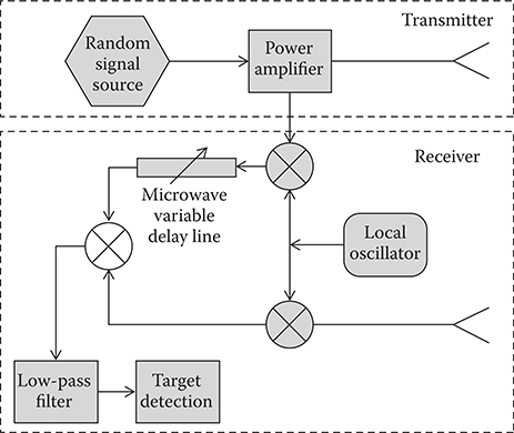
FIGURE 6.1
Simplified architecture of a correlation receiver-based random signal radar using a microwave variable delay line at the IF frequency.

where T_int is the integration time. In the noiseless case, the maximum value of |R(τ)| is at τ = τ₀.

For the random signal radar, assume that x(t) is a white stationary Gaussian random process with autocorrelation function R_xx(τ). Thus, the output of the correlation receiver given by Equation 6.2 is also a random process. The mathematical expected value of Equation 6.2 is

\begin{matrix} E [R (τ)] = & E [\int_{0}^{T_{i n t}} y (t) x^{*} (t - τ) d t] \\ = & \int_{0}^{T_{i n t}} E [y (t) x^{*} (t - τ)] d t \\ = & \int_{0}^{T_{i n t}} (A_{σ} E [x (t - τ_{0}) x^{*} (t - τ)] + E [n (t) x^{*} (t - τ)]) d t \\ = & A_{σ} \int_{0}^{T_{i n t}} R_{X X} (τ - τ_{0}) d t + \int_{0}^{T_{i n t}} E [n (t) x^{*} (t - τ)] d t . \end{matrix} (6.3)

$\begin{matrix} E [R (τ)] = & E [\int_{0}^{T_{i n t}} y (t) x^{*} (t - τ) d t] \\ = & \int_{0}^{T_{i n t}} E [y (t) x^{*} (t - τ)] d t \\ = & \int_{0}^{T_{i n t}} (A_{σ} E [x (t - τ_{0}) x^{*} (t - τ)] + E [n (t) x^{*} (t - τ)]) d t \\ = & A_{σ} \int_{0}^{T_{i n t}} R_{X X} (τ - τ_{0}) d t + \int_{0}^{T_{i n t}} E [n (t) x^{*} (t - τ)] d t . \end{matrix} (6.3)$

As the noise n(t) is uncorrelated with the radar waveform, the second term in Equation 6.3 is zero. Then, we have

E [R (τ)] = A {}_{σ}T_{i n t} R_{x x} (τ - τ_{0}) . (6.4)

$E [R (τ)] = A {}_{σ}T_{i n t} R_{x x} (τ - τ_{0}) . (6.4)$

Since the maximum of autocorrelation R_xx(τ - τ₀) occurs when τ = τ₀, the target delay τ₀ can be estimated as

τ_{0} = \max_{τ} E [R (τ)] . (6.5)

$τ_{0} = \max_{τ} E [R (τ)] . (6.5)$

To examine the solutions to the random signal radar, we consider the following three special forms of transmitted signal x(t):

Ideal white Gaussian noise: For this case, the autocorrelation function R_xx(τ) is a Dirac function, and therefore E[R(τ)] is also a Dirac function. That means, this waveform has an ideal range resolution (as small as only one data sample). Unfortunately, such signal occupies unlimited signal bandwidth and cannot be used in practical applications.
Band-limited white Gaussian noise with rectangular power spectral density (PSD) envelope $| S_{xx} (f) | = rect (\frac{f - f_{0}}{B})$ $| S_{xx} (f) | = rect (\frac{f - f_{0}}{B})$ : Based on the Wiener-Khintchine theorem, the PSD of a random stationary signal equals the Fourier transform of the corresponding autocorrelation. Thus, the autocorrelation function R_xx(τ) has the form of the sinc function $R_{xx} (τ) = \frac{sin (π B τ)}{π τ} e^{- j 2 π f_{0} τ} = B sinc (π B τ) \cdot e^{- j 2 π f_{0} τ}$ $R_{xx} (τ) = \frac{sin (π B τ)}{π τ} e^{- j 2 π f_{0} τ} = B sinc (π B τ) \cdot e^{- j 2 π f_{0} τ}$ , where the mainlobe occurs at τ = 0, and with some sidelobes. The first sidelobe is −13dB lower than the mainlobe.
Random stationary noise signal with Gaussian-shaped PSD envelope $| S_{xx} (f) | = e^{- {(\frac{f - f_{0}}{B})}^{2}}$ $| S_{xx} (f) | = e^{- {(\frac{f - f_{0}}{B})}^{2}}$ : According to the Wiener-Khintchine theorem, we can derive that the autocorrelation function $R_{xx} (τ) = \sqrt{π} B \cdot e^{- {(π B τ)}^{2}} \cdot e^{- j 2 π f_{0} τ}$ $R_{xx} (τ) = \sqrt{π} B \cdot e^{- {(π B τ)}^{2}} \cdot e^{- j 2 π f_{0} τ}$ has the form of Gaussian function. That means there is no range sidelobe at all, which makes it very attractive for radar applications. However, note that in practical cases, we have only one realization of the random signal combined with limited integration time. The PSD cannot have an ideal Gaussian shape. So random signal radar normally has high-range sidelobes. To get around this, Xu and Narayanan introduce a sidelobe suppression method based on median and apodization filtering [44].

6.1.3.2 Spectrum Analysis Receiver

As mentioned in Section 6.1.3.1, the microwave variable delay line is a key component in the correlation receiver of a random signal radar. Unfortunately, in the past, manufacturing of the microwave variable delay line proved very difficult. In 1968, Poirier [19] proposed another implementation architecture called “spectrum analysis radar,” which eliminated the microwave variable delay line. In this architecture, the detector adds the received target echo signal and the transmitted reference signal and uses spectrum analysis to detect the target. Figure 6.2 shows the simplified architecture of the spectrum analysis receiver-based random signal radar.

In the spectrum analysis receiver, the down-converted radar received signal y(t) is first added with the down-converted transmitted signal x(t). Following the notation used in Section 6.1.3.1, the sum of the received and transmitted signals becomes

s (t) = x (t) + y (t) = x (t) + A_{σ} x (t - τ_{0}) + n (t) . (6.6)

$s (t) = x (t) + y (t) = x (t) + A_{σ} x (t - τ_{0}) + n (t) . (6.6)$

Images

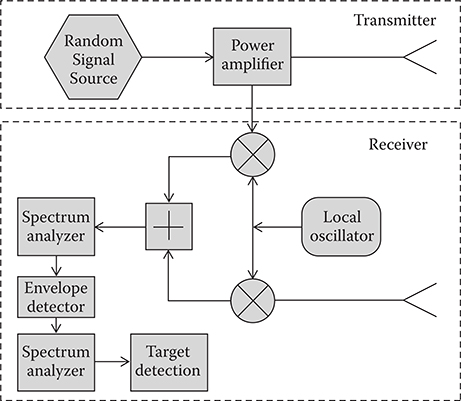
FIGURE 6.2
Simplified architecture of a spectrum analysis receiver-based random signal radar. This works by adding the received target echo signal and the transmitted reference signal. Target detection uses the spectrum analysis of the sum signal.

Its autocorrelation function is

\begin{matrix} R_{s s} (τ) = & E [s (t) s^{*} (t - τ)] \\ = & E [(x (t) + A_{σ} x (t - τ_{0}) + n (t)) (x^{*} (t - τ) + A_{σ}^{*} x^{*} (t - τ - τ_{0}) + n^{*} (t - τ)] \\ = & R_{X X} (τ) + A_{σ}^{*} R_{X X} (τ + τ_{0}) + R_{x n} (τ) + A_{σ} R_{X X} (τ - τ_{0}) + | A_{σ} |^{2} R_{X X} (τ) + A_{σ} R_{xn} (τ - τ_{0}) \\ = & + R_{n x} (τ) + R_{n x} (τ + τ_{0}) + R_{nn} (τ) . \end{matrix} (6.7)

$\begin{matrix} R_{s s} (τ) = & E [s (t) s^{*} (t - τ)] \\ = & E [(x (t) + A_{σ} x (t - τ_{0}) + n (t)) (x^{*} (t - τ) + A_{σ}^{*} x^{*} (t - τ - τ_{0}) + n^{*} (t - τ)] \\ = & R_{X X} (τ) + A_{σ}^{*} R_{X X} (τ + τ_{0}) + R_{x n} (τ) + A_{σ} R_{X X} (τ - τ_{0}) + | A_{σ} |^{2} R_{X X} (τ) + A_{σ} R_{xn} (τ - τ_{0}) \\ = & + R_{n x} (τ) + R_{n x} (τ + τ_{0}) + R_{nn} (τ) . \end{matrix} (6.7)$

As the noise n(t) is uncorrelated with the radar waveform, we have

R_{s s} (τ) = (1 + | A_{σ} |^{2}) R_{x x} (τ) + A_{σ}^{*} R_{X X} (τ + τ_{0}) + A_{σ} R_{x x} (τ - τ_{0}) + R_{n n} (τ) . (6.8)

$R_{s s} (τ) = (1 + | A_{σ} |^{2}) R_{x x} (τ) + A_{σ}^{*} R_{X X} (τ + τ_{0}) + A_{σ} R_{x x} (τ - τ_{0}) + R_{n n} (τ) . (6.8)$

The first spectrum analyzer output is the PSD of the summed signal s(t). Based on the Wiener-Khintchine theorem, the PSD of s(t) is equal to the Fourier transform of its autocorrelation function R_ss(τ):

\begin{matrix} S_{s s} (f) = & F T [R_{s s} (τ)] \\ = & (1 + | A_{σ} |^{2} + A_{σ}^{*} e^{j 2 π f τ_{0}} + A_{σ} e^{- j 2 π f τ_{0}}) S_{X X} (f) + S_{nn} (f) \\ = & (1 + | A_{σ} |^{2}) S_{X X} (f) + | A_{σ} | \cos (2 π f τ_{0} - θ_{σ}) S_{X X} (f) + S_{nn} (f), \end{matrix} (6.9)

$\begin{matrix} S_{s s} (f) = & F T [R_{s s} (τ)] \\ = & (1 + | A_{σ} |^{2} + A_{σ}^{*} e^{j 2 π f τ_{0}} + A_{σ} e^{- j 2 π f τ_{0}}) S_{X X} (f) + S_{nn} (f) \\ = & (1 + | A_{σ} |^{2}) S_{X X} (f) + | A_{σ} | \cos (2 π f τ_{0} - θ_{σ}) S_{X X} (f) + S_{nn} (f), \end{matrix} (6.9)$

where |A_σ| and θ_σ are the amplitude and phase of target reflectivity A_σ, respectively. S_xx(f) is the PSD of transmitted signal x(t) and S_nn(f) is the PSD of noise n(t). Note that the PSD of the summed signal s(t) consists of three terms: the first term is the PSD of the transmitted signal, the second term is the modulated PSD of the transmitted signal, and the third term is the PSD of noise.

We assume that the PSD of transmitted signal S_xx(f) occupies a bandwidth B, and the receiver bandwidth is equal to the transmitted signal bandwidth. In this case, the Fourier transform of the envelope of S_ss(f), that is, the output of the second spectrum analyzer in Figure 6.2, can be approximated as

F T [| S_{s s} (f) |] = c_{0} δ (u) + c_{1} δ (u - τ_{0}) + c_{1} δ (u + τ_{0}), (6.10)

$F T [| S_{s s} (f) |] = c_{0} δ (u) + c_{1} δ (u - τ_{0}) + c_{1} δ (u + τ_{0}), (6.10)$

where c₀ and c₁ are constants and δ(·) is the Fourier transform of the PSD envelope of the transmitted signal |S_xx(f)|. If the PSD of the transmitted signal has a rectangular envelope, δ(·) will be a sinc function. The target time delay τ₀ can be estimated as the position of peaks in Equation 6.10, and therefore, the range of target R₀ can be calculated by R₀ = cτ₀/2.

Note that as in Equation 6.10, even for a single target, two symmetric spectral peaks will be generated at the output of the second spectrum analyzer. Thus, this spectrum analysis receiver is also called “double spectral processing receiver” in some literatures [49].

The spectrum analysis receiver illustrated in Figure 6.2 can easily measure the distance of the stationary target without using the microwave variable delay line. However, it also has some drawbacks. First, when the target is moving, the Doppler frequency will induce loss of detection in the output of the spectrum analyzers. Second, when multiple targets exist, the cross-terms between different targets will generate some ghost targets. To solve these problems, Schindler, Holt, and Pierce [20–23] presented a few improved architectures of the spectrum analysis receiver, where a Doppler-shifted local oscillator was used in the down-conversion of received signal, and the ranges/velocities of targets can be measured by a series of complicated microwave networks that are matched to different target Doppler frequencies. More detailed information about these improved spectrum analysis receivers can be found in the works [20–23].

6.1.3.3 Digital Receiver

The correlation receiver and the spectrum analysis receiver were proposed about 50 years ago, where the target range and velocity measurements were implemented by using complicated analog microwave networks. Relatively, the correlation receiver possesses more advantages than the spectrum analysis receiver. However, the difficulties in manufacturing microwave variable delay lines restricted the implementation of the correlation receiver for random signal radar. In recent years, benefiting from the rapid development of electronic technology, the high-speed, high-resolution ADC and the digital signal-processing (DSP) devices enable implementation of the digital receiver. Figure 6.3 illustrates a simplified architecture of a digital receiver-based random signal radar, where the down-converted transmitted reference signal and received echo signal are digitized and fed into the digital signal processor, and all subsequent processing is implemented in the digital signal processor by software. Using the ADCs with very high sampling rate, the transmitted and the received signals can even be digitized in RF stage directly, which can further simplify the radar receiver architecture [only including receiving antenna, bandpass filter (BPF), ADC, and signal processor]. It should be noted that when very low-bit ADC is adopted to improve the signal-processing rate and reduce cost, the ideal correlation function will be distorted and additional processing loss will be induced [66,67]. However, such drawbacks can be ignored for most ADCs with 8-bit resolution or more.

Images

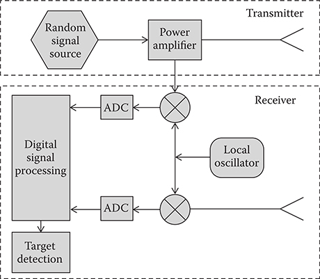
FIGURE 6.3
Simplified architecture of a digital receiver-based random signal radar. This implementation digitizes the down-converted transmitted reference signal and received echo signal, which then go into the digital signal processor. A digital processor of software does all subsequent processing.

Basically, compared with the conventional analog receiver, the digital receiver has the following two main advantages:

With the much simpler architecture, the digital receiver can avoid some undesired effects caused by microwave devices (such as nonlinearity and intermodulation) and has less system errors, and thus it can achieve more robust working performance.
The processing is implemented in the digital signal processor software, which gives much more flexibility than that of the conventional analog receiver. Using advanced signal-processing algorithms greatly enhances the target-detection performance. Moreover, the digital receiver allows for continuous improvements through reprogramming.

6.1.4 Processing Schemes for Random Signal Radar

Next, we briefly introduce two typical processing schemes for the moving target range/velocity measurement using random signal radar.

We still assume that x(t) is the random signal transmitted by the radar and y(t) is the received signal. For a moving point target at the range R₀ and with velocity υ, the instantaneous target range is R(t) = R₀ + υt. The received signal y(t) can be written as

\begin{matrix} y (t) = & A_{σ} x (t - τ) + n (t) \\ = & A_{σ} x (t - \frac{2 R (t)}{c}) + n (t) \\ = & A_{σ} x (t - \frac{2 R_{0}}{c} - \frac{2 v t}{c}) + n (t) \\ = & A_{σ} x ((1 - \frac{2 v}{c}) t - \frac{2 R_{0}}{c}) + n (t), \end{matrix} (6.11)

$\begin{matrix} y (t) = & A_{σ} x (t - τ) + n (t) \\ = & A_{σ} x (t - \frac{2 R (t)}{c}) + n (t) \\ = & A_{σ} x (t - \frac{2 R_{0}}{c} - \frac{2 v t}{c}) + n (t) \\ = & A_{σ} x ((1 - \frac{2 v}{c}) t - \frac{2 R_{0}}{c}) + n (t), \end{matrix} (6.11)$

where A_σ is the target complex reflectivity and n(t) is the undesired receiver noise. If α = 1 - (2υ/c) and τ₀ = 2R₀/c, then Equation 6.11 simplifies to

y (t) = A_{σ} x (α t - τ_{0}) + n (t) . (6.12)

$y (t) = A_{σ} x (α t - τ_{0}) + n (t) . (6.12)$

Thus, to implement the matched filter processing to the received signal y(t), the cross-correlation of the received signal y(t) and the delayed and time-compressed copy of transmitted signal x(α₁t - τ_r) becomes

C_{y x} (α_{r}, τ_{r}) = \int_{0}^{T_{i n t}} y (t) x^{*} (α_{r} t - τ_{r}) d t . (6.13)

$C_{y x} (α_{r}, τ_{r}) = \int_{0}^{T_{i n t}} y (t) x^{*} (α_{r} t - τ_{r}) d t . (6.13)$

In practical applications, the parameters α_r and τ_r are varied until the correlation maximum is found, from which the target range and velocity can be estimated by R = (c + v) τ/2 and v = c(1 - α_r)/(1 + α_r). The cross-correlation of Equation 6.13 can be computed using efficient fast Fourier Transform (FFT) processing.

Equation 6.13 does a two-dimensional (2D) joint processing, and it does not make any assumption or limitation on the radar signal and target parameters. To illustrate this feature, consider a simulation conducted for a UWB random signal acoustic radar. The assumed radar system and target parameters are listed in Table 6.1.

In this simulation, the transmitted acoustic signal occupies a bandwidth from 0 Hz to 10 kHz, and the relative bandwidth is equal to 1. This definitely qualifies as a UWB radar. On the other hand, the target velocity 5 m/s is not so “small” relative to the propagation velocity of sound 340 m/s, which is equivalent to a target velocity of 4.4 × 10⁶ m/s for a microwave radar. Thus, the time compression effect in the received target signal is significant. Theoretically, the range resolution of this UWB random signal acoustic radar is ΔR = v_sound/2B = 340/(2 × 10⁴ = 0.017) m, and the Doppler resolution is Δf_d = 1/T_int = 10 Hz, which can be translated to a velocity resolution of 0.34 m/s (for the centre frequency of 5kHz). Figure 6.4 depicts the 2D-joint-processing results obtained by Equation 6.13, where two target peaks are prominently detected, and their positions indicate the estimated range/velocity values of respective targets.

The range/velocity estimation described by Equation 6.13 is based on finding the delay τ_r, and compression factor α_r of the reference signal, giving a correlation peak. The computational load of this processing is very high, particularly when long integration time is adopted to achieve high-velocity resolution. A simpler way, just like the range-Doppler processing in conventional pulse radar, is to divide the 2D joint processing of Equation 6.13 into sequential steps. First, a number of correlation computations are performed with different delays, forming the range cells. The integration time at each correlation processing should be selected significantly shorter than the period time of the maximum Doppler shifts of target signals. Repeating the correlation procedure for a sequence of transmitted/received random signals generates a signal vector whose phase time variation depends on the Doppler shift of the target. Then, by applying FFT processing in each range signal vector, the output of different Doppler cells can be obtained. A great advantage of this processing is that the efficient FFT algorithm can be applied in Doppler processing, which greatly reduces the computational load. Also, the range correlation procedure may also be implemented by FFT, making use of the fact that the convolution of two signals can be computed from the inverse Fourier transform of the product of their Fourier transforms. However, it should be noted that the bandwidth of the transmitted waveform will degrade the Doppler resolution of the target [45]. Thus, this two-step range-Doppler processing technique is only applicable for narrowband random signal radar. While in the previous 2D joint processing, by a stepwise approach of v_r to the true v value, the velocity resolution will not be affected by the signal bandwidth. Thus, for the wideband random signal radar, the previous 2D joint processing should be applied.

TABLE 6.1
Simulation Parameters for an UWB Random Signal Acoustic Radar

Images

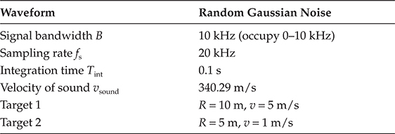
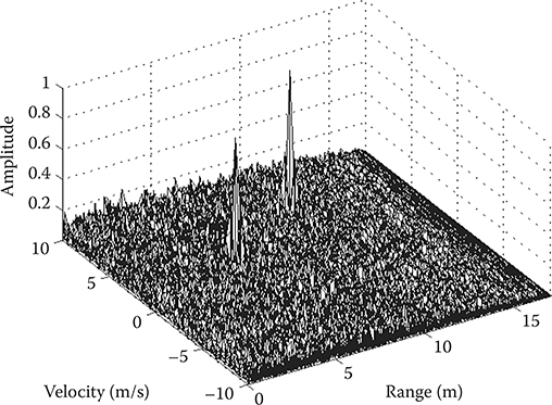
FIGURE 6.4
Simulated target detection result of a UWB random signal acoustic radar (Target 1: R = 10 m, v = 5 m/s; Target 2: R = 5 m, v = 1 m/s).

6.2 Combination of UWB and Random Signal Radar

Conventional narrowband waveforms limit the information capacity of the radar system. Increasing the system’s information capacity requires expanding its band of frequencies. For the many advantages provided by radars of expanded bandwidth, researchers are now actively pursuing UWB radar worldwide. Generally, the waveform of the UWB radar has one of the following two characteristics: a short duration or a complicated waveform with many frequency components. The carrier-free pulse with a very short duration is the simplest UWB waveform. However, the generation and control of high-power uniform carrierfree pulse train is difficult to achieve in practice. The other type of UWB waveform is the compressed CW/pulse signal that contains many frequency components. Compressed CW/pulse signals attain a large bandwidth by modulating the transmit signal instead of decreasing its time duration, such as the LFM signal. Compared with the carrier-free impulse signal, the main advantage of a compressed waveform is that the UWB can be achieved without decreasing the pulse width and thus the energy in the pulse. However, if the required bandwidth is too large, the linearity of frequency sweep in a chirp signal is not easy to maintain, and the range sidelobes will be affected. The random signal radar has no such requirement, and it is relatively easier to implement the UWB signal [68]. In this section, we will first briefly introduce the three generation methods of random signal, and then investigate the combination of the UWB technique and the random signal radar, that is, how to implement the ultrawide bandwidth for different random signal radar waveforms.

6.2.1 Random Signal Generation

The random signal radar requires a controllable random signal generator as a key component. The generated random signal should have a specific spectrum output within the required bandwidth and should satisfy some statistical characteristics such as stationary, ergodic, Gaussian, and with zero mean. Basically, the generation of random signal includes the following approaches:

Dedicated microwave noise devices, such as a back-biased diode working in the avalanche discharge mode. This simple and easy approach generates a random signal that closely resembles the white noise.
Chaotic oscillators, that is, dynamical chaotization of oscillations in microwave self-oscillators or nonlinear oscillatory circuits. With this approach, the chaotic signal can be generated for a specified bandwidth with properties very close to that of true random noise. Lukin and his coworkers did a lot of work on this, and many chaos generators were developed for VHF/UHF, X, Ka, and W bands [58].
Digital generators (or software generators): Pseudorandom number generation is a mature technique that has been widely used in many areas. The computer-generated pseudorandom number can be easily converted to an analog signal as the transmitted waveform of a random signal radar [the present digital-to-analog converter (DAC) or arbitrary waveform generator (AWG) can support the output signal bandwidth up to gigahertz, which is enough for the UWB random signal radar implementation]. However, we must recognize that the computer does not generate a truly random signal. The resulting signal has an inherently periodic nature with a very long period. Random signal radar applications require only that the generated pseudorandom signal does not appear periodic within the processing or integration time. We can easily satisfy this requirement. As an example, a 64-bit pseudorandom signal generator has a theoretical period of 2⁶⁴ ≈ 1.84 × 10¹⁹. If one random number is generated every 1 ns (which corresponds to a bandwidth of 1 GHz), the sequence will repeat after 584 years.

6.2.2 UWB Carrier-Modulated Random Signal Radar

6.2.2.1 Random Noise Radar

The random noise radar uses a band-limited microwave random noise transmitted waveform. A microwave noise source followed by a BPF can directly generate the random noise radar signal. Alternatively, the transmitter can generate the signal at some baseband and then upconvert it to RF. Figure 6.5a and b illustrates these two easily implemented UWB signal-generation methods.

We can model the transmitted random noise signal as the following complex form:

S (t) = S_{b} (t) e^{j 2 π f_{0} t}, (6.14)

$S (t) = S_{b} (t) e^{j 2 π f_{0} t}, (6.14)$

where f₀ is the centre frequency of the transmitted signal and S_b(t) is a complex stationary Gaussian process with zero mean and bandwidth B, which can also be expressed as

S_{b} (t) = A (t) e^{j ψ_{0} (t)}, (6.15)

$S_{b} (t) = A (t) e^{j ψ_{0} (t)}, (6.15)$

where A(t) is the Rayleigh-distributed amplitude and ϕ₀(t) is the uniformly distributed random phase between [-π,π]. Substituting Equation 6.15 in Equation 6.14, we have

S (t) = A (t) e^{j (2 π f_{0} t + ϕ_{0} (t))} . (6.16)

$S (t) = A (t) e^{j (2 π f_{0} t + ϕ_{0} (t))} . (6.16)$

Thus, we can model this random noise waveform as a signal with both amplitude and frequency/phase modulation.

Narayanan at the University of Nebraska-Lincoln developed a typical example of the UWB random noise radar [35]. Figure 6.6 shows the simplified block diagram of the Narayanan’s radar. This system uses the noise source OSC1 built from a commercially available component that contains a noise diode, a BPF, and an amplifier. This produces a signal with a Gaussian amplitude distribution and an average output level of 0 dBm in the 1-2-GHz frequency range. The noise source output splits into two equal in-phase components in the power divider PD1. One of the outputs goes to a broadband power amplifier AMP1 before transmission. The second output of PD1 connects to a combination of a fiber-optic fixed delay line DL1 and a digitally controlled variable delay line DL2. The fixed delay line sets the minimum range to the target. The variable delay line can program delays from 0 to 19.968 ns in 0.156 ns steps. The delay line output mixes with the output of a 160 MHz phase-locked oscillator OSC2 in a lower sideband upconverter MXR1. The upconverter has an output in the 0.84-1.84 GHz frequency range, which feeds upcon-verter MXR2. The 1-2 GHz received signal provides the second input to mixer MXR2. Since the two mixer inputs are shifted by 160 MHz, the output of mixer MXR2 is always at 160 MHz. The 160 MHz output of MXR2 goes through a 160 MHz BPF with a bandwidth of 5 MHz and feeds into the I/Q detector for processing. Narayanan first applied this UWB random noise radar system to detection of targets buried in the soil [35,36] and ISAR imaging [41,42]. Later modifications lowered the transmitter frequency to operate at 250-500 MHz for measurement of foliage penetration [38]. In all these experimentations, the UWB random noise radar performed well and produced many interesting results.

Images

FIGURE 6.5
Implementation methods of a random noise radar waveform. (a) RF noise source generation. (b) Baseband noise source generation.

Images

FIGURE 6.6
Simplified block diagram of Narayanan’s UWB random noise radar. Note the fixed and variable delay lines DL1 and DL2. (Adapted from Narayanan, R.M. et al., Opt. Eng., 37, 1855-1869, 1998. With permission from SPIE, © 1998.)

Note that the random noise radar’s transmitted waveform is band-limited random noise with a nonconstant envelope. These qualities make it highly susceptible to the nonlinearities in radar architectural components. For example, if the frequency response of the power amplifier has nonlinear characteristics in the band of interest, then the performance of the random noise radar will worsen significantly. This feature also restricts the employment of random noise radar for long-range applications. In the long-range radar system, the power amplifier often works in the saturation mode to achieve a stable high-power transmission output. For this case, the random noise signal with a nonconstant envelope will not always operate in the saturation mode and produce performance anomalies. Thus, the random noise radar that directly uses a band-limited random noise waveform is only suitable for low-power and short-range applications.

6.2.2.2 Random Frequency Modulation Radar

Another type of random signal radar waveform uses a sine wave with frequency or phase modulation by a low-frequency random signal. Such a waveform has a constant envelope and is applicable for high-power, long-range applications. A voltage-controlled oscillator (VCO) controlled by a baseband noise signal provides the random frequency modulations. The mathematical model of random frequency modulation signal can be expressed as

S_{f} (t) = \exp (j (2 π f_{0} t + \int_{0}^{t} f (x) d x)), (6.17)

$S_{f} (t) = \exp (j (2 π f_{0} t + \int_{0}^{t} f (x) d x)), (6.17)$

where f(t) is the frequency modulation random signal, which is a Gaussian variable with zero mean and autocorrelation function $R_{f} (τ) = σ_{f}^{2} ρ_{f} (τ)$ $R_{f} (τ) = σ_{f}^{2} ρ_{f} (τ)$ . The autocorrelation function of random frequency-modulated signal S_f(t) can be expressed as [64]

R_{S_{f}} (τ) = \exp (- 4 π^{2} \int_{0}^{τ} (τ - x) R_{f} (x) d x) = exp (- 4 π^{2} σ_{f}^{2} (τ - x) ρ_{f} (x) d x)) . (6.18)

$R_{S_{f}} (τ) = \exp (- 4 π^{2} \int_{0}^{τ} (τ - x) R_{f} (x) d x) = exp (- 4 π^{2} σ_{f}^{2} (τ - x) ρ_{f} (x) d x)) . (6.18)$

Based on the Wiener-Khintchine theorem, we can show that the root-mean-square (rms) bandwidth of random frequency-modulated sine wave is equal to the rms value of frequency modulating signal σ_f and is independent of the shape of the correlation function ρ_f(τ). When σ_f is large, R_{S_f} (τ) has a shorter correlation time than ρ_f (τ), which means that the modulated output has a larger bandwidth than the modulation random signal. In addition, the sidelobes of the frequency-modulated output signal will also be lower than that of the modulation random signal [64]. Theoretically, if the modulation random signal has a sinc-shape autocorrelation function, the sidelobe of output waveform can be completed eliminated.

In the 1980s, Liu and his coworkers at Nanjing University of Science and Technology in China developed and introduced an experimental random frequency modulation CW radar [24–26]. Figure 6.7 shows a simplified block diagram of the Liu’s system. This system adopted a special technique in the correlation receiver to avoid using a microwave variable delay line. The received signal is directly mixed with the transmitted signal. For a moving target at zero range, the mixer output will be a single Doppler signal. For a moving target at a certain range, the mixer output will be a signal with spread spectrum whose center frequency is equal to the target-produced Doppler shift. The mixed signal is then split into two channels and passed into two BPFs. Their respective pass-bands are f₂ - f₁ and f₃ - f₂, where f₃ > f₂ > f₁. The signal of each channel passes through the BPF, power detector, and log-amplifier. The final radar output is the difference of the two channels, whose voltage is inversely proportional to the target range. Liu and his coworkers also presented a compounded random frequency modulation radar system, which introduced a low-frequency sine wave into the frequency modulation to suppress the strong short-range clutter [26].

Images

FIGURE 6.7
Simplified block diagram of Liu’s random frequency modulation radar. The final radar output is the difference of the two BPF and power detector channels, whose voltage is inversely proportional to the target range. (Adapted from Liu, G. et al., “Random FM-CW radar and its ECCM,” Proc. 1986 Int. Conf. Radar, China, 155-160, November 1986; Liu, G. et al., “Noise FM-CW radar system,” Proc. 1989 Int. Symp. Noise Clutter Reject. Radars Imaging Sensors, Japan, 578-583, November 1989; Liu, G. et al., “Design of noise FM-CW radar and its implementation,” IEE Proc.—Part F: Radar and Signal Process, 138, 5, 420-426, September 1991.)

6.2.2.3 Random Phase Modulation Radar

The mathematical model of random phase modulation signal can be expressed as

S_{P} (t) = exp (j (2 π f_{0} t + θ (t)), (6.19)

$S_{P} (t) = exp (j (2 π f_{0} t + θ (t)), (6.19)$

where θ(t) is the phase modulation random signal, which is a Gaussian variable with zero mean and autocorrelation function $R_{θ} (τ) = σ_{θ}^{2} ρ_{θ} (τ)$ $R_{θ} (τ) = σ_{θ}^{2} ρ_{θ} (τ)$ . The autocorrelation function of random phase modulation signal S_p(t) can be expressed as [64]

R_{S_{p}} (τ) = \exp (- σ_{θ}^{2} (1 - ρ_{θ} (τ))) . (6.20)

$R_{S_{p}} (τ) = \exp (- σ_{θ}^{2} (1 - ρ_{θ} (τ))) . (6.20)$

Based on the Wiener-Khintchine theorem, it can be derived that the rms bandwidth of random phase-modulated sine wave is increased by a factor σ_θ compared with the rms bandwidth of the phase modulating random signal. The sidelobe level of the phase-modulated output is also significantly reduced compared with that of the modulation random signal [64].

Note that in the above discussion, we assume a continuous random phase modulation. An alternative technique is binary phase modulation, that is, the phase of carrier signal jump between 0 and π, which is randomly controlled by the sign of the Gaussian noise signal θ(t). For this case, the sidelobe improvement is (π/2)² or 4 dB compared to the modulating signal [64].

In the 1990s, Liu and Gu [28–30] developed the experimental random binary phase modulation CW radar shown in the simplified block diagram of Figure 6.8. This radar has an operating frequency of 35 GHz and an average transmitting power of 180 mW. The subpulse width for one-phase coding is 500 ns, which corresponds to a range resolution of 75 m. In this system, the received signal is down-converted to baseband and is digitized by the ADC card. Then the data are transferred to the digital signal processor to implement the pulse compression, Doppler processing, constant false alarm rate (CFAR), and target display in real time. Although this radar is not a UWB system and does not possess very outstanding target-detection performance, it is still a significant contribution because (a) the architecture of the digital receiver is implemented and the concept of random binary phase modulation is verified and (b) the generation of the coded waveform and subsequent processing are programmable, and it is very easy to change different codes (random or pseudorandom) and compare their performance.

Images

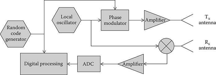
FIGURE 6.8
Simplified block diagram of Liu’s random binary phase modulation CW radar using random binary-phase coded modulation. The 500-ns subpulse width for one phase corresponds to a range resolution of 75 m. (Adapted from Liu, G. and Gu, H., “A comparison between random and pseudorandom binary phase-coded CW radar system,” Proc. 1991 Int. Conf. Radar, China, 390-392, October 1991; Liu, G. and Gu, H., “Random binary phase coded CW radar system,” Proc. 1996 Int. Conf. Radar, China, 254-258, October 1996; Gu, H. and Liu, G., “A new kind of radar—Random binary phase-coded CW radar,” Proc. 1997 Natl. Radar Conf., Syracuse, NY, 202-206, May 1997.)

6.2.2.4 Random Interrupted CW Radar

To date, almost all random signal radars work in the CW mode, which transmits a continuous waveform and has a peak transmission power equal to the average power. The CW design reduces the requirements of the power amplifier and can dramatically reduce the total system cost compared with the pulse-type systems. Furthermore, the CW radar’s low-peak transmission power will also significantly lower the interception probability by the enemy, which makes the radar an attractive feature in the modern battlefield. However, the CW radar has a critical drawback because of the signal leakage between the transmitter and the receiver, which restricts its high-power applications for long-range target detection. To solve this problem, Khan and Mitchell [69] proposed the concept of interrupted CW waveform, where a CW waveform is gated on and off with a well-defined sequence, and an echo signal is received only during the quiet period after the transmitter has been turned off. In the Khan and Mitchell’s concept, the linear frequency modulated continuous wave (FMCW) is interrupted many times within a frequency sweeping period. Gu et al. [70] introduced another interruption method using a periodic square wave for the general CW radar, whose operating time sequence is plotted in Figure 6.9.

Figure 6.9a shows the periodic square wave used as the gating signal to control the transmitting and receiving time sequences, where T₁ is for transmission and T₂ is for reception. The total waveform repetition period is T = T₁ + T₂, and normally T₁ ≤ T₂. The maximum duty cycle of such interrupted CW waveform is 50% when T₁ = T₂. Figure 6.9b shows the transmitted CW waveform after interruption, and Figure 6.9c shows the target return signal with a time delay τ₀. The target return signal received by the radar is shown in Figure 6.9d, where a part of the target return signal is gated off and the remaining time width of the received pulse is T_d. The variation of the received pulse width T_d versus the target time delay τ₀ is plotted in Figure 6.10. This feature has two advantages and one disadvantage. The advantages are as mentioned below.

First, the direct path leakage signal with zero time delay will be eliminated by the gating, which solves the aforementioned problem of signal leakage in CW radars. Second, the pulse width of the received signal T_d is proportional to the target delay when τ₀ < T₁, as shown in Figure 6.10. Based on the free-space propagation loss equation, we have known that the received signal power is inversely proportional to R⁴, where R is the target range. For this interrupted CW radar, if T₁ is equal to the maximum time delay of the target echo, then the pulse width of the received signal is proportional to the target range R. Thus, the total received signal power is inversely proportional to R³, which can significantly reduce the dynamic range of the received signal power.

Images

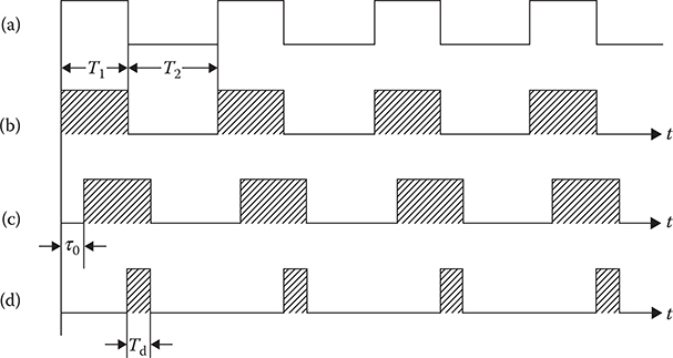
FIGURE 6.9
Operating time sequence of Gu’s CW radar waveform interrupted by a periodic square wave: (a) Gating signal to control transmitting T₁ and receiving times T₂. (b) The transmitted CW waveform after interruption. (c) The target return signal with a time delay τ₀. (d) The received target return signal where a part of the target return signal is gated off and the remaining time width of received pulse is T_d. (Adapted from Gu, H. et al., Acta. Electron. Sinica, 26, 12, 7-11, 1998 (in Chinese).)

Images

FIGURE 6.10
Variation of received pulse width versus target time delay in Gu’s CW radar waveform interrupted by a periodic square wave. (Adapted from Gu, H. et al., Acta. Electron. Sinica, 26, 12, 7-11, 1998 (in Chinese).)

The disadvantage is that the received target signal after interruption is only partially correlated with the transmitted signal, which may affect the sidelobe level of the matched filter processing output.

To verify the performance of the interrupted CW waveform, we ran numerical simulations that assumed a random frequency modulation CW signal with a bandwidth of 50 MHz, whose baseband spectrum is shown in Figure 6.11. Figure 6.12a shows one period of the transmitted waveform (real part) after periodic square wave interruption with a duty cycle of 50%. It means that the first 500 samples are for transmission and the next 500 samples are for reception. We assume a stationary point target with a time delay of 200 samples. The received target echo signal after interruption is shown in Figure 6.12b. Figure 6.13 shows the cross-correlation result of the transmitted reference signal and the received target echo signal. It can be seen that the time delay of the target signal is correctly detected at the 200th sample, and the highest sidelobe is at about -12dB. For comparison, Figure 6.14 depicts the autocorrelation of the transmitted reference signal, where the highest sidelobe is at about -16dB. As expected, owing to the partial correlation between the transmitted reference signal and the interrupted received signal, the sidelobe level in Figure 6.13 is slightly higher than that in Figure 6.14.

Images

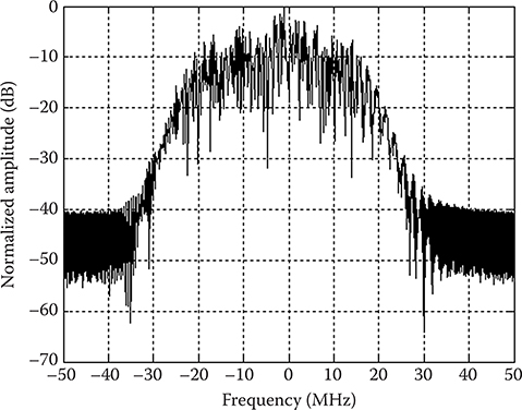
FIGURE 6.11
The interrupted CW radar simulation assumed a random frequency modulation signal with a bandwidth of 50 MHz.

Images

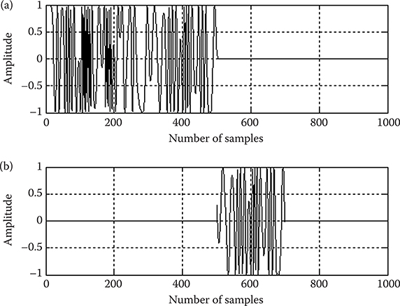
FIGURE 6.12
The interrupted CW radar simulation: (a) Transmitted signal and (b) Received signal.

Images

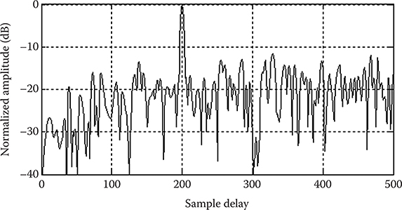
FIGURE 6.13
The interrupted CW radar simulation results in the cross-correlation of the transmitted reference signal and the interrupted received signal.

Images

FIGURE 6.14
The interrupted CW radar simulation results in the autocorrelation of the transmitted reference signal.

Note how the interrupted CW waveform has totally different performance characteristics from the normal pulse waveform, although the waveforms look very similar. First, for an ideal point target, the received target echo signal of the normal pulse radar appears as a delayed copy of the transmitted waveform. In the interrupted CW radar, the received target echo signal is not only a delayed copy of the transmitted waveform, but also a part of the signal is interrupted (as a reminder, this feature can improve the dynamic range of the received signal). Second, the normal pulse radar has a “blind zone” at short range, which is equal to the time width of transmitted pulse, whereas the interrupted CW radar does not have a blind zone and can detect targets at a very short range.

By combining the random frequency/phase modulation and the interrupted CW techniques, we can totally solve the problem that restricts the high-power application of the random signal radar. However, the previous interruption method using a periodic square wave is not very ideal for its periodic nature. The repetition frequency of the square wave cannot be too low; otherwise ambiguity in Doppler measurement will occur. To avoid this ambiguity, the repetition period T should be short, which will cause a “blind spot” problem because at the position τ₀ = T, the target echo signal is totally gated off. Gu and Su [34] proposed a “dual-random” interrupted CW waveform that can solve the problem of fixed blind spots. In this “dual-random” system, the radar carrier signal is first modulated by the random binary phase coding, and then the modulated CW waveform is interrupted randomly, not periodically. That means including two different random modulations. Figure 6.15 depicts the operating time sequence of this “dual-random” waveform. Similar to the interruption method using periodic square wave, the randomly interrupted waveform can also eliminate the signal leakage at zero range. However, different from the periodically interrupted waveform where the range blind spot is fixed, the randomly interrupted waveform has random range blind spots. Subsequent statistical processing can remove the blind spot. It is similar to the pulse-Doppler radar using different staggered PRFs to remove the range ambiguity. This dual-random interrupted CW radar concept is indeed unique and innovative, which solves the two major problems that restrict the high-power application of the random signal radar, that is, (a) the random phase modulation waveform with constant envelope allows the use of a high-power amplifier and (b) the random interruption technique eliminates the signal leakage at zero range and also solves the problem of fixed blind spot.

Gu et al. developed an experimental dual-random interrupted CW radar system based on this concept [34]. Figure 6.16 depicts its simplified block diagram. This system is based on the previous random binary phase modulation CW radar [28–30], where one more random code generator is added to control the interruption of the random binary phase-modulated CW waveform. To achieve high isolation, two T/R modules are used in the transmitting channel and one T/R module is used in the receiving channel. The transmitting and receiving channels are connected to the antenna through a circulator, which moves energy from an input port to the antenna and from the antenna to the T/R3 output port. The isolation of each T/R module is 60 dB, and the isolation of circulator is 30 dB. It can be calculated that when the radar is receiving a signal, the isolation between the transmitting and receiving channels is 60 dB + 60 dB + 30 dB = 150 dB. That means that the signal leakage from the transmitter can be attenuated for about 150 dB to the receiver input. This solves the problem of signal leakage from the transmitter to the receiver. When the radar transmits, the isolation between the transmitting and receiving channels is 60 dB + 30 dB = 90 dB, which makes the receiver well protected.

Images

FIGURE 6.15
Operating time sequence of Gu’s “dual-random” interrupted CW radar waveform. This approach solves two major problems of high-power random signal radar. (Adapted from Gu, H. and Su, W., “A new quasi-continues wave radar,” Proc. 9th Chinese Natl. Radar. Symp., China, 23-26, April 2004 (in Chinese).)

Images

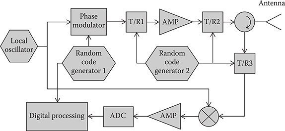
FIGURE 6.16
Simplified block diagram of Gu’s dual-random interrupted CW radar. (Adapted from Gu, H. and Su, W., “A new quasi-continues wave radar,” Proc. 9th Chinese Natl. Radar. Symp., China, 23-26, April 2004 (in Chinese).)

6.2.3 UWB Carrier-Free Impulse Radar with Random Coding

Carrier-free impulse is another type of the UWB waveform. To achieve high range resolution, the pulse width of a carrier-free waveform must be very short, which restricts the energy of the transmitted signal. Conventional microwave radars can achieve high-range resolution by using a good pulse-compression technique. This produces the equivalent of a narrow pulse by frequency or phase modulation of the pulse with large time-width. However, we cannot apply frequency or phase modulation to the UWB carrier-free impulse waveform. To solve this problem, Hussain proposed a random polarity coding technique, where a large number of carrier-free pulses coded by a pseudorandom noise sequence can provide sufficient energy (average power) for reliable target detection while achieving high range resolution [71].

We assume an UWB carrier-free rectangular pulse signal

\begin{matrix} Ω (t) = E \cdot rect (\frac{t}{Δ T}), & 0 \leq t \leq Δ T \end{matrix}, (6.21)

$\begin{matrix} Ω (t) = E \cdot rect (\frac{t}{Δ T}), & 0 \leq t \leq Δ T \end{matrix}, (6.21)$

where E is the amplitude of the pulse and ΔT is the pulse width. A carrier-free pulse waveform s(t) coded by a given binary sequence can be represented by a train of properly weighted and shifted rectangular pulses:

s (t) = Σ_{n = 0}^{N - 1} a_{n} Ω (t - n T_{D}) = E Σ_{n = 0}^{N - 1} a_{n} \cdot rect (\frac{t}{Δ T} - n D), (6.22)

$s (t) = Σ_{n = 0}^{N - 1} a_{n} Ω (t - n T_{D}) = E Σ_{n = 0}^{N - 1} a_{n} \cdot rect (\frac{t}{Δ T} - n D), (6.22)$

where {a_n, n = 0, 1, . . . , N − 1} is the selected binary code sequence, T_D is the unit time delay, and D = T_D/ΔT. Note that T_D is not necessarily confined to be a single pulse width ΔT, that is, D can be larger than 1. Here 1/D serves as the duty cycle. Increasing the parameter D can shift the range sidelobes of the autocorrelation function away from the mainlobe and create gaps between any two adjacent sidelobes. However, the transmitted signal power will decrease simultaneously. Figure 6.17 shows an example of a carrier-free pulse waveform coded by a 13-digit Barker sequence and its autocorrelation function where D = 1. Figure 6.18 shows the case where D = 5. For this UWB carrier-free coded impulse waveform, we can select the proper pulse width to achieve the required range resolution and select the proper code length to provide sufficient transmitting energy. The matched filter response for the carrier-free coded waveform is a function of the nominal bandwidth Δf = 1/ΔT (which specifies the range resolution), the duty cycle 1/D (which governs the range ambiguity), the code length N (which limits the total signal energy and affects the amplitude of range sidelobes), and the selected code characters {a_n, n = 0, 1, . . . , N - 1}.

Hussain proposed a hardware implementation architecture for the generation of a carrier-free coded waveform based on a passive pulse expansion network shown in Figure 6.19 [71]. The pulse expander consists of a pulse generator (PG), a tapped-analog delay line (TAD), pulse-shaping amplifiers (AMP), controllable switches (SW), and synchronization circuits (SYNCH). In Hussain’s system, the network can transmit carrier-free coded waveforms with the time variation of the signal given in Equation 6.22 with length N = 8. The network can be extended to generate coded waveforms of longer lengths by increasing the number of stages of TAD, AMP, and SW.

Theoretically, the carrier-free waveform can use both random and pseudorandom binary codes. The autocorrelation function of truly random codes approximates a Dirac function, which makes an ideal radar waveform. However, the ideal random code has infinite period, where the code length has to be truncated for practical use. The range sidelobes of the truncated random code autocorrelation function may be high, and the excessively high sidelobes can appear as false targets. Thus, further processing is required to suppress them. Different from the truly random code, the pseudorandom codes have finite periods, have easy implementations, and offer flexible selection of the code length. For example, the maximum-length code is a typical pseudorandom code that can be easily generated by a linear feedback shift register. The autocorrelation function of the maximal-length codes has constant sidelobes, which is very suitable for this carrier-free coded waveform. Hussain also mentioned the use of complimentary codes [71]. Complimentary codes consist of a pair of sequences with the same length whose autocorrelation functions have sidelobes equal in magnitude but opposite in sign. The sum of the two autocorrelation functions has no sidelobes. However, in practical applications, the two sequences must be separated in time, frequency, or polarization, which results in decorrelation of radar returns and hence complete sidelobe cancellation may not occur.

Images

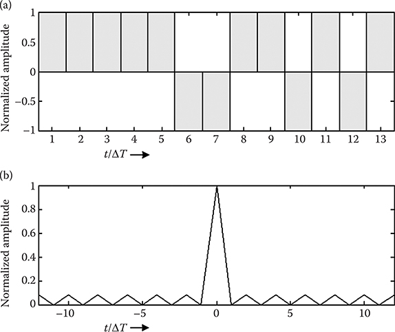
FIGURE 6.17
Carrier-free coded waveform: (a) 13-digit Barker codes, D = 1. (b) Autocorrelation function.

Images

FIGURE 6.18
Carrier-free coded waveform: (a) 13-digit Barker codes, D = 5. (b) Autocorrelation function.

Images

FIGURE 6.19
Hussain’s hardware implementation of a carrier-free pulse expansion system for the generation of a UWB carrier-free coded waveform. (Hussain, M.G.M., “Principles of high-resolution radar based on nonsinusoidal waves—Part 1: Signal representation and pulse compression,” IEEE Trans. Electromag. Compatibil., 31, 4, 359-368, November 1989, © 1989 IEEE.)

6.3 Advantages of UWB Random Signal Radar

Benefiting from large bandwidth and random signal modulation, the UWB random signal radar possesses many special advantages over conventional radars. For example, an easily implemented random UWB signal can achieve very high range resolution. The resulting random signal radar can extract a fine target signature and alleviate the influences of multipath or clutter. On the other hand, conventional pulse radars suffer from ambiguities in range and Doppler (velocity) measurement. For the UWB random signal radar, the random nature of the waveform totally eliminates the constraints on range/Doppler ambiguities and can detect very long range targets with very high velocities. In this section, we investigate another three attractive advantages of the UWB random signal radar, namely (a) anti-RFI capability, (b) LPI property, and (c) EMC. These features make the UWB random signal radar a winner in both the military and civilian operating environments [68,72].

6.3.1 Anti-RFI Capability

Since the UWB radar occupies much broader bandwidth than the conventional radars and often operates at lower frequency bands, it is extremely vulnerable to the RFI from other illuminator sources. A typical example is the foliage penetration radar. To attain the capability of foliage penetration, the radar has to operate at VHF-UHF bands. Unfortunately, the VHF-UHF portion of the spectrum is already in heavy use by other services such as radio/television broadcasting and mobile communications. To achieve high range resolution, the radar waveform must share its spectrum with unwanted interference signals. Thus, the anti-RFI performance is one of the critical issues for UWB radar applications. In Sections 6.3.1.1 and 6.3.1.2, we compare the target detection performance of the conventional radar and the random signal radar in the presence of strong narrowband and wideband RFI, respectively.

6.3.1.1 Narrowband RFI

For UWB radars, most RFIs from other illuminator sources have narrow bandwidths, such as FM radio, analog TV, analog wireless communication (like the walkie-talkie), and the second generation of digital cellular mobile communications, which normally have band-widths of less than 100 kHz. To examine this problem, we investigate the effects of narrowband RFIs on the performance of different radar waveforms. We shall select the typical LFM waveform and the random noise waveform for comparison.

We assume that the signal has a 30 MHz bandwidth, the complex sampling rate is 50 MHz, the integration time is 100 μs, and the environment contains two discrete narrowband RFI sources. The range point spread function (PSF), which describes the response of a target after matched filtering, is adopted as a reference to evaluate the performance of the two waveforms. Figure 6.20 depicts the comparison results of the baseband spectrum and PSF of the LFM signal, with and without narrowband RFI contamination. It can be seen that the sidelobes of the PSF are significantly increased when the LFM signal is contaminated by the narrowband RFIs. Figure 6.21 shows the corresponding results for one recurrence of a random noise waveform. We can find that the contamination effect of the narrowband RFI on the PSF of the random noise waveform is very trivial, and no significant difference can be seen for the results with and without narrowband RFI contamination. Comparing the RFI-contaminated PSFs in Figures 6.20 and 6.21, the sidelobe level of random noise waveform is slightly lower than that of the conventional LFM waveform for about 1-2 dB. Note that due to the random nature of the waveform, the PSF sidelobes of the random noise signal are randomly distributed, which can be further suppressed by averaging some number of recurrences; however, such averaging will not reduce the sidelobe level of the deterministic signal such as LFM. Figure 6.22 shows the results of random noise waveform after an average of 10 recurrences, where the random noise signal has at least a 5 dB lower sidelobe level than the LFM signal.

Images

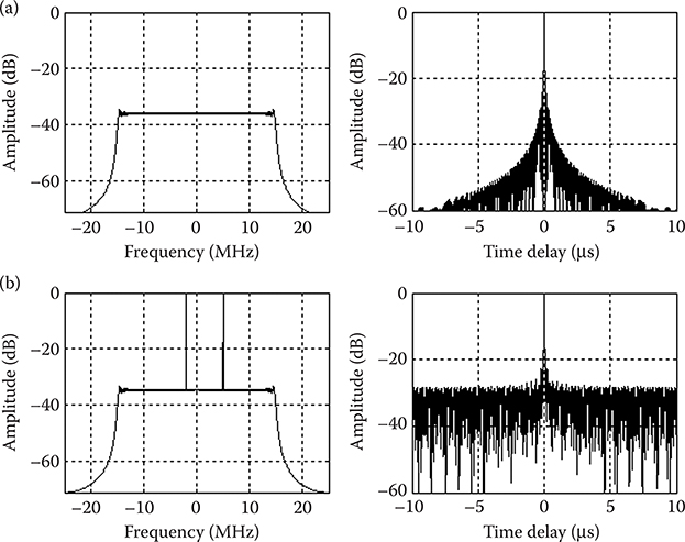
FIGURE 6.20
Comparison of spectrum and PSF of LFM waveform: (a) Without and (b) with narrowband RFI contamination.

Figures 6.20 through 6.22 show the comparison results for the case of two discrete narrowband RFIs. Other researchers performed and reported similar analyses in other literatures. Xu et al. [36] showed the comparison results for the case of dense RFI environment, where a 10 dB lower sidelobe level can be achieved by the random noise waveform. Xu and Narayanan [37] analyzed the integrated sidelobe ratio (ISLR) and peak sidelobe level (PSL) as the function of percentage bandwidth coverage of RFI. Mogila et al. [73] demonstrated the different effects of monochromatic RFI on SAR imaging for the LFM waveform and random noise waveform, respectively. All of these results prove that the random signal waveform is immune to the impact of the narrowband RFIs, compared with the conventional deterministic radar waveform such as LFM.

Images

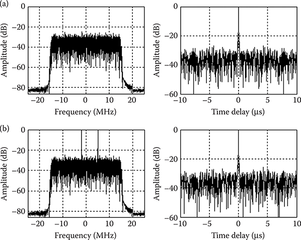
FIGURE 6.21
Comparison of spectrum and PSF of random noise waveform (one recurrence): (a) Without and (b) with narrowband RFI contamination.

Images

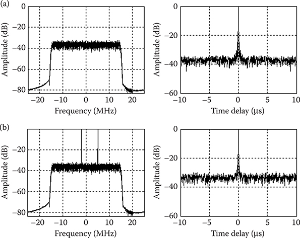
FIGURE 6.22
Comparison of spectrum and PSF of random noise waveform (10-recurrence averaging): (a) Without and (b) with narrowband RFI contamination.

6.3.1.2 Wideband RFI

In recent years, more new commercial broadcasting and communication systems started operation, such as digital audio/video broadcasting (DAB/DVB), worldwide interoperability for microwave access (WiMAX) network, and the third generation of digital cellular mobile communication. The signals emitted by these service systems possess very wide bandwidth (from a few MHz to several tens of MHz) and act as new challenges for the applications of UWB radar. However, this issue has not been addressed in public literature. This section will present some simulation results to compare the effects of wideband RFI on the PSF of LFM signal and random noise signal.

We still assume the same radar parameters as those used in Section 6.3.1.1, and a simulated DVB signal with 8-MHz bandwidth is injected as a wideband RFI. The processing results for the LFM signal are illustrated in Figure 6.23. We can find that the influence of wideband RFI on the PSF of LFM signal is more significant than the narrowband RFI. The wideband RFI-contaminated PSF shown in Figure 6.23 has about 8 dB higher sidelobes than the narrowband RFI-contaminated PSF shown in Figure 6.20. Figures 6.24 and 6.25 depict the results of random noise waveform for the cases of 1- and 10-recurrence averaging, respectively. Owing to the effect of wideband RFI, the sidelobe level of the PSF of random noise waveform increases by about 7 dB. However, comparing the RFI-contaminated results in Figures 6.23 and 6.25, the random noise waveform is still superior to the LFM signal for about 5-7 dB lower PSL. These results conclude that compared with the conventional LFM waveform, the random signal waveform is also immune from the impact of the wideband RFI.

Images

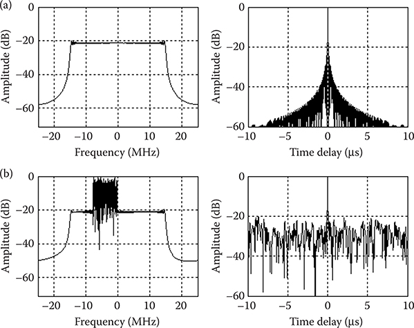
FIGURE 6.23
Comparison of spectrum and PSF of LFM waveform: (a) Without and (b) with wideband RFI contamination.

Images

FIGURE 6.24
Comparison of spectrum and PSF of random noise waveform (one recurrence): (a) Without and (b) with wideband RFI contamination.

Images

FIGURE 6.25
Comparison of spectrum and PSF of random noise waveform (10-recurrence averaging): (a) Without and (b) with wideband RFI contamination.

6.3.2 Low Probability of Interception

In the modem battlefield, the increased use of electronic support measures (ESM), radar warning receivers (RWR), and antiradiation missile (ARM) systems brings serious threats to the survival of the radar. These make LPI an important requirement to modern radars. In order to hide themselves from the interception by enemy RWRs, radar systems should work silently. That is to say, the operating range, R_R, of the radar system should be larger than that of the enemy’s RWR, R_I. To evaluate the LPI performance quantitatively for radar systems, Schleher defined the range factor α = R_I/R_R and analyzed the relationship between the range factor and radar parameters [74]. Generally, based on the requirements of reducing range factor, and therefore, improving LPI performance, radar systems should have a wide transmit antenna pattern, reduce the noise temperature and loss in radar receiver, choose a lower operating frequency, and transmit waveforms with large time-bandwidth product. These conclusions apply to all radars and should be taken into account in the system design.

Besides the above factors, reducing the radar system’s peak transmission power provides another effective technique to improve the LPI performance. Thus, for the same average transmission power and maximum target detection range, the CW radar has better LPI performance than the conventional pulse radar. As mentioned, the random signal radar measures target range by the correlation processing between the target echo signal and the delayed transmit signal, and therefore, this makes it very suitable for CW operating mode. To overcome the signal leakage problem in CW radars, we can apply the technique of interrupted CW waveforms, as presented in Section 6.2.2.4.

From the waveform’s point of view, we can reduce the range factor and enhance the LPI performance significantly by choosing a proper waveform modulation to reduce the required input SNR for the radar receiver and simultaneously bring a great loss to the enemy’s intercept receiver. In a radar receiver, increasing integration time can enhance coherent integration and target SNR. However, the enemy intercept receiver may not always achieve sufficient coherent integration, which depends on the properties of the intercepted radar waveform. Conventional radars transmit identical pulses or recurrences of a waveform, which can be easily integrated and identified by the intercept receiver. To prevent integration in the RWR, we can design the radar to transmit a randomly time varied and nonperiodic waveform. The intercept receiver will see a noiselike signal and cannot perform coherent integration without some a priori knowledge of the signal characteristics. Thus, even with very long integration time, the intercept receiver will have a difficult time detecting and identifying the random signal radar waveform. Figure 6.26 shows the simulated Fourier spectrums of LFM waveform when 1, 10, and 100 recurrences are intercepted, respectively. It is assumed that there are 200 samples in one recurrence, and the original SNR is 10 dB. We can find that increasing the observation time and integrating more recurrences significantly enhances the SNR of the LFM waveform, which makes it easier to intercept. Figure 6.27 illustrates the results of random frequency-modulated waveform. Owing to its time-varied and nonperiodic natures, the SNR of random frequency-modulated waveform remains at the same level when different numbers of recurrences are integrated. The probability of interception for the random radar waveform cannot be increased by extending the observation time. Note that in Figure 6.27 we have selected the random frequency modulation waveform as an example. Similar results for comparing the LFM and the random noise waveform were obtained in the work [75]. All these prove that the random signal radar has an excellent LPI property.

Images

FIGURE 6.26
Fourier spectrums of LFM waveform after integrating: (a) 1, (b) 10, and (c) 100 recurrences.

Note that even if you can intercept a random signal radar waveform, then you still have a major problem in identifying, replicating, and jamming it. Given this introduction, we shall consider the typical repeater jammer. After intercepting the radar signal, the repeater jammer must be able to identify its waveform, then predict and replicate it with additional regular or random time delays. Apparently, the radar using a periodic, deterministic waveform such as the LFM is especially susceptible to this type of jamming, since the jammer can construct a good estimate of LFM signal parameters and use it to jam the radar system with forged replicas. In recent years, the use of a digital RF memory (DRFM) device has greatly facilitated the implementation of the repeater jammer and has enhanced its capabilities. In the DRFM-based jammer system, the intercepted radar signal is first digitized and recorded into RF memory. Analyzing the recorded signals helps estimate the interrupted waveform parameters and generate a false target response in digital form. Finally, this jammer converts the digital signal to an analog format and transmits it toward the victim radar to produce a false target indication. However, this scenario will not work for the random signal radar, because (a) the random signal radar waveform parameters are very difficult to identify and estimate, particularly for CW or randomly interrupted CW random waveforms and (b) each intercepted and stored signal sample in the repeater jammer will become obsolete quickly as the random signal radar waveform unpredictably varies with time.

Garmatyuk and Narayanan [76] investigated the property of random noise waveform that can complicate the signal identification/emulation in the repeater jammer. This assumes that we know the central frequency and bandwidth of the radar signal, and the jammer works by continuous estimation of the instantaneous frequency of the intercepted radar signal. The jammer will try to estimate the deviation of the signal’s frequency and adjust its own frequency to produce the jamming signal. To test the performance of this model, the author generated the band-limited random noise (BLRN) and LFM chirp (LFMC) waveforms and fed them into the above jammer model. Figure 6.28a and b shows an example of signal identification/prediction, whereas Figure 6.28c shows the normalized cross-correlation functions between the jammer-predicted and real radar waveforms. Notice how easily you can predict the LFM signal, while the random frequency variations in BLRN signal effectively prevent signal identification and prediction.

Images

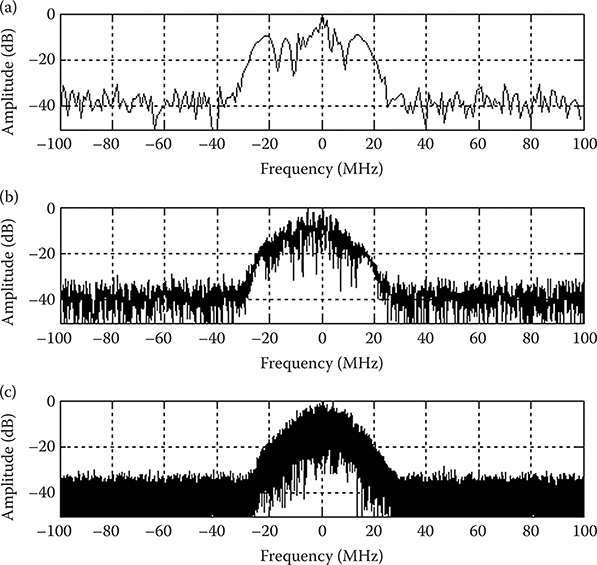
FIGURE 6.27
Fourier spectrums of random frequency-modulated waveform after integrating: (a) 1, (b) 10, and (c) 100 recurrences.

6.3.3 Electromagnetic Compatibility

In February 2002, the Federal Communications Commission (FCC) officially released the authorization that permits the marketing and operation of UWB systems for commercial use. This will make more UWB radar systems available for civilian applications. When civilian radars go into mass production and application, many systems may work in the same area simultaneously. This will require suppressing the electromagnetic interference among such systems so that each system can work normally without mutual interference. Therefore, civil UWB radars require a high standard of EMC performance. We know that the available spectrum resources have limits, and we cannot realistically assign a different portion of the available spectrum for each UWB radar system. Thus, we must inevitably share frequencies among multiple systems. Conventional radars using deterministic waveforms (such as LFM) and sharing the same frequency band cannot work simultaneously in the same area. Otherwise they will interfere with each other significantly and generate ghost targets. By using the nature of random modulation, random signal radars can share the same frequency band and operate simultaneously in close proximity. Thayaparan et al. [75] presented a series of simulation results to compare the mutual interference effects for LFM and random noise waveforms. In this section, we use the automotive collision warning radar as an example to show the superior EMC performance of random signal radars.

Images

FIGURE 6.28
Signal identification/prediction performance: (a) Predicated LFM signal. (b) Predicated random noise signal. (c) Cross-correlation function of predicated and real radar signals. (Garmatyuk, D.S. and Narayanan, R.M., “ECCM capabilities of an ultrawideband bandlimited random noise imaging radar,” IEEE Trans. Aerospace Elect. Sys., 38, 1243-1255, October 2002, © 2002 IEEE.)

Recently, there has been an upsurge of research on automotive collision-warning radar. We suppose that in a given area we have multiple car radars and there is the potential for interference among them. Before producing automotive collision warning radars as commercial products, we must overcome the principal problem of high false alarm rates. Among all the factors leading to false alarm, the oncoming vehicle’s interference on the opposite direction lane will pose the most serious condition. The host radar will receive a strong interference signal from the approaching radar. Furthermore, the same operation frequency and transmitting waveform make the situation worse. To prevent this mutual interference, designers of automotive collision-warning radars have paid increased attention to random/pseudorandom signal modulation. For example, Lukin studied random noise waveform in automotive collision-avoidance applications [56–57]. Detlefsen et al. [77] developed a collision warning radar prototype based on a pseudonoise (PN-code) phase-modulated signal. Kajiwara [78] proposed an m-sequence phase modulation pulse waveform for the collision warning radar. In that work, the correlation processing of random/pseudorandom modulated signal ensures that the target signal be detected correctly while suppressing the interference.

Based on Kajiwara’s work [78], Liu and Zhang proposed an improved multiple-slope m-coded stepped FMCW waveform [72,79], as shown in Figure 6.29a. The radar transmitting cycle has two (or more) slope pairs divided into four segments A-D. Segments A and C correspond to an up-chirp signal, and B and D correspond to a down-chirp signal, where f_c indicates the carrier frequency. Using different frequency modulation (FM) sweep limits enhances multiple-target detection capability and reduces the false alarm probability. For A-D, each segment comprises N steps of short burst. The duration of each burst is T_p. For each segment, a unique m-sequence is also modulated. The time-width of a code in this m-sequence is equal to the width of an FM step, that is, T_p, as shown in Figure 6.29b. For each segment (up-chirp or down-chirp) of the slope pair, the echo signal from a target is homodyne-detected and I/Q sampled. According to the principle of high-resolution radar profile synthesis, an inverse Fourier transform operation can synthesize the target profile from the samples. Figure 6.30 shows the proposed block diagrams of the multiple-slope m-coded stepped FMCW radar system and signal processor. More detailed description about range/velocity measurement and multiple-targets detection algorithms can be seen in [79]. Next, we will show the excellent EMC performance of the proposed waveform.

Images

FIGURE 6.29
Multiple-slope m-coded stepped FMCW waveform (a) Frequency variation of the multiple-slope stepped FMCW waveform and (b) m-sequence modulated transmitting bursts. (Liu, G. et al., “Random signal radar—A winner in both the military and civilian operating environments,” IEEE Trans. Aerospace Elect. Sys., 39, 489-498, April 2003, © 2003 IEEE.)

Images

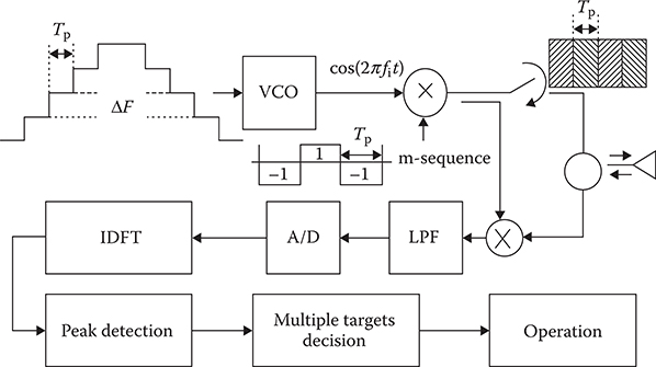
FIGURE 6.30
Proposed block diagram of multiple-slope m-coded stepped FMCW radar system and signal processor. (Liu, G. et al., “Random signal radar—A winner in both the military and civilian operating environments,” IEEE Trans. Aerospace Elect. Sys., 39, 489-498, April 2003, © 2003 IEEE.)

The use of m-sequence-modulated waveform can ensure correct detection in a strong interference environment. In the case of the vehicle radar, assume that all vehicles in the frontal area have different m-sequences and that every vehicle transmits the similar triangle waveform modulated by a unique m-sequence. When the host radar receives an echo signal consisting of interference and a useful target signal, receiver homodyne detects the combined signal first. The host m-sequence demodulates the interference, and the resulting phase of the sampled sequence should be random. On the contrary, after demodulation by the host m-sequence, the resultant phase of the useful target signal will be linear. Subsequent coherent processing can largely remove the effects of interference. Thus, other radars will not interfere with the host radar unless the interfering radar uses the same m-sequence coding.

A computer simulation verifies the superior EMC performance of this waveform. Suppose the radar carrier frequency f_c = 77 GHz, the number of bursts in every slope N = 128, frequency spacing ΔF = 0.5 MHz, the duration of each burst T_p = 1 ns, and the length of m-sequence is 127 bits. Figure 6.31 shows the resulting range profiles for various signal-to-interference ratios (SIR) with the following conditions: (a) for a target range of 50 m, (b) when the received signal includes a strong interference signal from a random range, and (c) the interference signal has the same waveform as the transmitted signal but with different m-sequence modulation. Figure 6.31a and b correspond to the results with and without m-sequence modulation, respectively. Figure 6.32 shows the unwrapped phases of the target signal and interference. We can see that after the correlation processing with the host reference signal, the phase of the target signal is linear, while the phase of the interference signal is random. The m-sequence modulation can effectively suppress the interference component, which greatly enhances the EMC performance of the automotive collision warning radar.

It is worth noting that the true random waveform has better EMC performance than the pseudorandom waveform. Liu et al. introduced an experiment of EMC performance comparison between random binary-phase-coded (RBPC) and pseudorandom binary-phase-coded (PBPC) waveforms [72,80]. Figure 6.33 shows the experimental scene. The jammer is positioned 3.2 m away from the radar, within the sidelobe direction of the radar receiving antenna. The false target is positioned at 7.5 m from the radar, within the mainlobe direction of the radar receiving antenna. This false target locates in the first range bin of the radar with a Doppler offset of 6 kHz. Table 6.2 gives the operating parameters of the radar, and Table 6.3 shows the jammer characteristics. The experiment used four types of jamming signals including aiming jamming, random FM jamming, RBPC modulation jamming, and PBPC modulation jamming. Figure 6.34 shows the jamming signal spectra. The experimenters performed a total of 100 observations to calculate the detection probability and false alarm probability for the two types of radar signals. Table 6.4 shows the experimental results. It clearly shows that compared with the pseudorandom signal modulation, the true random signal modulation has better resistance to external interferences. Thus, it has better EMC performance and suitability for civilian applications.

Images

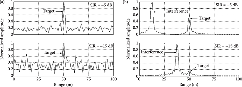
FIGURE 6.31
Radar range profiles for various signal-to-interference ratios (SIR). (a) With m-sequence modulation. (b) Without m-sequence modulation. (Liu, G. et al., “Random signal radar—A winner in both the military and civilian operating environments,” IEEE Trans. Aerospace Elect. Sys., 39, 489-498, April 2003, © 2003 IEEE.)

Images

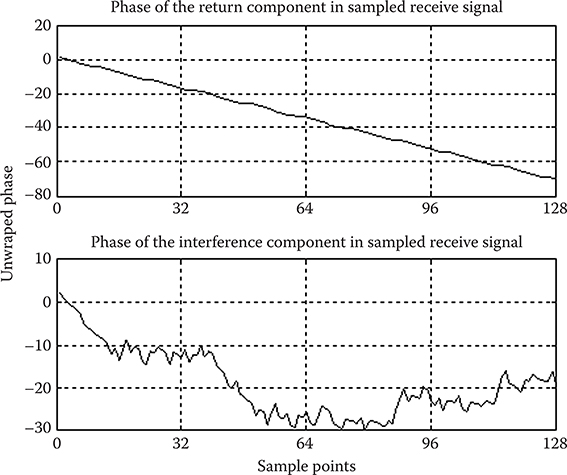
FIGURE 6.32
Unwrapped phases of the target signal and interference. (Liu, G. et al., “Random signal radar—A winner in both the military and civilian operating environments,” IEEE Trans. Aerospace Elect. Sys., 39, 489-498, April 2003, © 2003 IEEE.)

Images

FIGURE 6.33
Experimental setup for comparing the EMC performances of RBPC and PBPC radar waveforms. (Liu, G. et al., “Random signal radar—A winner in both the military and civilian operating environments,” IEEE Trans. Aerospace Elect. Sys., 39, 489-498, April 2003, © 2003 IEEE.)

TABLE 6.2
EMC Performance Comparison—Radar System Operating Parameters

Images

6.4 Applications of UWB Random Signal Radar

The UWB random signal radar system can provide excellent capabilities for unambiguous range and Doppler measurements with high resolution and accuracy, and superior anti-RFI, LPI, and EMC performance, which promises success in both the military and civilian operating environments [68,72]. So far, random signal radars have been successfully used in the following applications:

TABLE 6.3
EMC Performance Comparison—Jammer Operating Parameters

Images

FIGURE 6.34
Spectra of the EMC test jamming signals: (a) Aiming jamming. (b) Random FM jamming. (c) RBPC modulation jamming. (d) PBPC modulation jamming. (Liu, G. et al., “Random signal radar—A winner in both the military and civilian operating environments,” IEEE Trans. Aerospace Elect. Sys., 39, 489-498, April 2003, © 2003 IEEE.)

Radar fuze systems [81–84]
Detection of underground and buried objects [35–36]
Detection of targets obscured by foliage and walls [37–39]
Short-range SAR imaging [37,39,40,51-53]

TABLE 6.4
EMC Performance Comparison—Experimental Results

Images

Remote monitoring of structural changes [54,55]
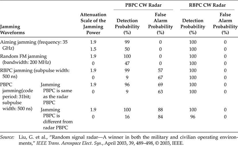
ISAR imaging measurements in microwave anechoic chamber [41,42,59]
Impulse function measurements for moving targets [60–62]
Car collision warning/avoidance and intelligent traffic control systems [56,57]

Next, we show some typical examples of the UWB random signal radar in various application scenarios.

6.4.1 Detection of Buried Objects

Detection of buried objects under the ground is an important task for both the military and civilian radar systems. Narayanan and his coworkers at the University of Nebraska-Lincoln developed an experimental UWB polarimetric random noise radar for this purpose [35,36]. The simplified block diagram and brief introductions about this system have been presented in Section 6.2.2.1. Table 6.5 summarizes the system specifications. Narayanan et al. used this system to gather data from an assortment of buried objects in a sand box (3.5 m long, 1.5 m wide, and 1 m deep). The experimenters scanned the radar antennas over the surface and collected continuous data. The buried targets included metallic and non-metallic objects of different sizes and shapes that mimicked land mines and other objects. Figure 6.35 shows photographs of the radar system and the trial setup.

From the raw data, the system produced four images corresponding to the copolarized received amplitude, cross-polarized received amplitude, and polarimetric phase difference between the orthogonally polarized received signals, and the depolarization ratio. To enhance the target detection and identification performance, the raw image data could then undergo postprocessing with an apodization filter, a median filter, and thresholding techniques and form Stokes matrix images and depolarization ratio images. As an example, Figure 6.36 shows the postprocessed images pertaining to two dissimilar metallic objects, a round metal plate 23 cm diameter × 2 cm thick, and a square metal plate 27 cm on each side × 1 cm thick, separated by 25.4 cm and buried at depths of 17.8 cm and 43.2 cm, respectively. The copolarized reflectivity image in Figure 6.36a clearly shows the presence of the two objects, but the objects do not appear in the cross-polarized reflectivity image. We can also clearly discern the presence of the object in three of the Stokes matrix images shown in Figure 6.36g through i. These results indicate that the polarimetric random noise radar does succeed in detecting metallic objects buried at depths as much as about 50 cm in relatively dry sandy soil.

TABLE 6.5
Specifications of Narayanan’s UWB Random Noise Radar for Detection of Buried Objects

Images

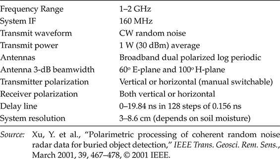
FIGURE 6.35
Photographs of Narayanan’s UWB random noise radar and trial setup for buried object detection. (Adapted from Narayanan, R.M. et al., Opt. Eng., 37, 1855-1869, 1998. With permission from SPIE, © 1998.)

Images

FIGURE 6.36
Processed images for two metallic plates. (a-d)—Raw images: (a) Copolarized magnitude, (b) cross-polarized magnitude, (c) polarimetric phase difference, and (d) depolarization ratio. (e-j)—Processed images: (e) Copolarization magnitude, (f) depolarization ratio, (g) S1, (h) S2, (i) S3, and (j) S4 images. (Adapted from Xu, Y. et al., “Polarimetric processing of coherent random noise radar data for buried object detection,” IEEE Trans. Geosci. Rem. Sens., 39, 467-478, March 2001, © 2001 IEEE.)

6.4.2 Short-Range SAR Imaging

Lukin and his coworkers at the Institute of Radio-Physics and Electronics, National Academy of Science of Ukraine, did numerous research works on the random noise radar. They developed a series of experimental random noise radar systems with ground-based SAR capabilities and obtained many promising measurement results for short-range surveillance of outdoor and indoor environments [51–53]. As an example, Figure 6.37 shows the simplified block diagram of Lukin’s ground-based X-band noise waveform SAR system for outdoor measurements. Table 6.6 lists the system specifications. In this system, the synthetic aperture is formed by the rotation of a 1.75 m-long boom, so it is called “arc-SAR.” The transmit waveform is a random noise pulse with a bandwidth of 500 MHz.

Images

FIGURE 6.37
Simplified block diagram of Lukin’s ground-based X-band noise waveform arc-SAR. (Courtesy of Professor K.A. Lukin.)

TABLE 6.6
Specifications of Lukin’s Ground-Based X-Band Noise Waveform Arc-SAR System

Images

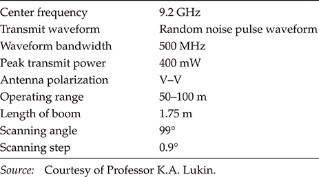
Figure 6.38 shows the system setup for outdoor SAR measurements. Lukin’s team mounted the radar beside a room window at the height of 20 m above the ground. Figure 6.39 shows the observed outdoor scene. Figure 6.40 shows the processed SAR image overlapped with ground truth. Most of the relevant features in the scene are clearly recognizable in the radar image. In particular, the layouts of the buildings, the metallic structure in the middle and right-hand side, and the reference corner reflector are correctly imaged.

Lukin and his coworkers also developed a ground-based Ka-band noise waveform SAR system for indoor measurements [52–53]. Figure 6.41 shows the simplified block diagram, and Figure 6.42 shows the system as built. This SAR system includes two pairs of TR antennas, two transmitters, and two receivers operating in adjacent frequency bands shifted by 500 MHz and having central frequencies 36.25 and 36.75 GHz, respectively. Besides, it also has two microcontroller-based synchronizers and a PC-based control, data acquisition, and processing unit. With different setups, this system works in monostatic, bistatic, and multiple input multiple output (MIMO) modes, and it can be used to verify various new concepts. Table 6.7 gives the detailed specifications of this versatile Ka-band SAR system. In addition, note that this system has a specially designed sliding-slot antenna shown in Figure 6.43 [52–53]. This concept uses the sliding motion of a radiating slot along a feeding waveguide, which forms the antenna aperture.

Images

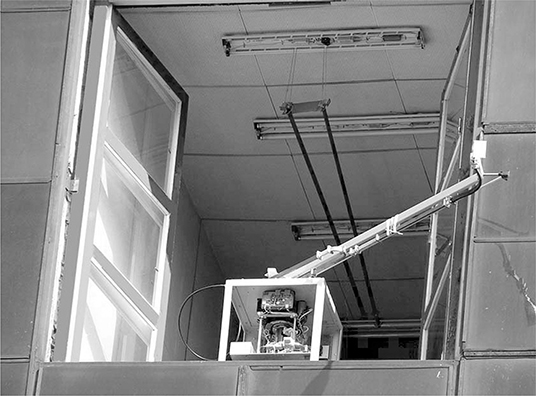
FIGURE 6.38
Photograph of Lukin’s ground-based arc-SAR measurement trial setup. (Courtesy of Professor K.A. Lukin.)

Images

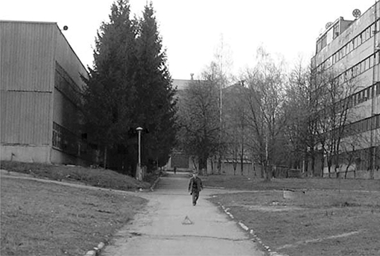
FIGURE 6.39
Photograph of Lukin’s arc-SAR outdoor trial scene. (Courtesy of Professor K.A. Lukin.)

Images

FIGURE 6.40
Lukin’s ground based arc-SAR outdoor scene processed measurement image. (Courtesy of Professor K.A. Lukin.)

Lukin and his coworkers performed indoor SAR imaging trials in a laboratory room with dimensions of 9.6 m × 5.7 m, in which some wooden tables with metal equipment stood along the walls, and the right wall had a few windows. They mounted the antennas at 1.6 m height and directed down toward the objects on the floor. The chosen bistatic configuration placed the antennas 2.5 m apart. Figure 6.44 shows a photograph of the test scene. Figure 6.45 shows the processed SAR image of the scene and a sketch of the room. As seen, the SAR image agrees well with the room topography, and we can see the two big targets clearly. This SAR system achieved range and azimuth resolutions of 0.4 and 0.06 m (at 5.65 m range), respectively.

To evaluate the temporal interferometric capabilities of this ground-based Ka-band SAR system, Lukin and his coworkers put two small targets (screw nuts) in the scene, as shown in Figure 6.46. First, they made a scan of the scene and generated the first SAR image, as shown in Figure 6.47a. In this normal SAR image, the two small targets were hidden by the sidelobes of strong scatterers and were not visible. Then, they made a second scan and generated the second image after shifting the two screw nut scatterers in range by 1 mm in opposite directions. They used these two SAR images to build the interferogram, which is shown in Figure 6.47b. Note that in Figure 6.47b an applied -30 dB-amplitude threshold helps avoid the influences from image areas with low reflectivity. The areas with reflectivity below -30dB appear in gray. Other parts of the interferogram have close to zero phase differences for most of the scatterers in the room. The yellow and blue small spots indicated by arrows correspond to the positions of the shifted small targets. The value of the phase difference detected for those targets agrees with the values calculated by the phase shifts of the signal caused by their true radial displacement.

Images

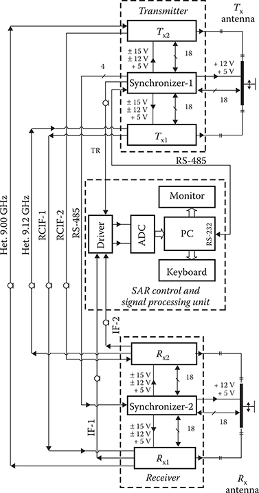
FIGURE 6.41
Simplified block diagram of Lukin’s ground-based Ka-band noise waveform SAR. (Lukin, K.A. et al., “Ka-band ground-based noise waveform SAR,” Proc. 6th Int. Kharkov. Symp. Phys. Eng. Microwaves, Millimeter and Submillimeter Waves and Workshop on Terahertz Technologies-MSMW’2007, 1, 59-164, June 2007, © 2007 IEEE.)

6.4.3 Remote Monitoring of Structural Changes

The indoor measurement results shown in Figure 6.47 demonstrated that the ground-based Ka-band noise waveform SAR system can detect very small changes in the scene by using a differential interferometry technique. We can apply this capability to remotely detect small changes on the surface of engineering structural objects. For example, Lukin and his coworkers measured movements in the interior of the bell tower of the UNESCO world heritage site at St. Sophia Cathedral in Kiev, Ukraine [54–55]. This section presents some interesting results for the measurements in the bell tower.

Figure 6.48 contains a photograph of the bell tower and the ground-based noise waveform SAR system. Lukin and his coworkers used the same radar system in the previous indoor measurements [53]; however, they employed it working in a monostatic mode and using a single-frequency channel. They placed the radar 22 m from the bell tower during the measurements and aimed the antennas at 54° upward from the horizontal. Over a 24-h period, they took measurements at 30 min or 1-h intervals depending on the time of the day. Figure 6.49 shows an example of the resulting SAR image. We can clearly see the building of bell tower and its parts such as peaks, windows, metal grates, dome, and cross in the image.

Images

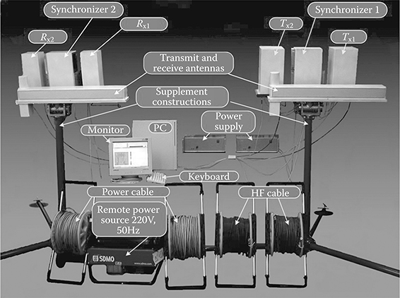
FIGURE 6.42
Lukin’s ground-based Ka-band noise waveform SAR system hardware. (Lukin, K.A. et al., “Ka-band ground-based noise waveform SAR,” Proc. 6th Int. Kharkov. Symp. Phys. Eng. Microwaves, Millimeter and Sub-millimeter Waves and Workshop on Terahertz Technologies-MSMW’2007, 1, 59-164, June 2007, © 2007 IEEE.)

TABLE 6.7
Lukin’s Ground-Based Ka-Band Noise Waveform SAR System Specifications

Images

By comparing the phases between the two SAR images obtained at different times, the differential interferograms can be generated. Figure 6.50 shows two examples of bell tower interferograms taken during nighttime and sunrise respectively, with a delay of 1 h. A threshold of 45 dB is shown by 50% gray in this figure. Green color corresponds to zero phase shifts, meaning there is no difference between two images. Apparently, night measurements showed rather high physical size stability of the bell tower, whereas some small shifts (up to 1 mm) can be spotted in the interferogram obtained during sunrise, which was supposed to be caused by the different heating of the building parts by the sun. Figure 6.51 shows the phase histogram calculated from the SAR data collected at night with constant temperature and absence of wind. The average width of the histogram of 3° gives a precision of displacement measurement of about 0.03 mm for the 8-mm wavelength.

Images

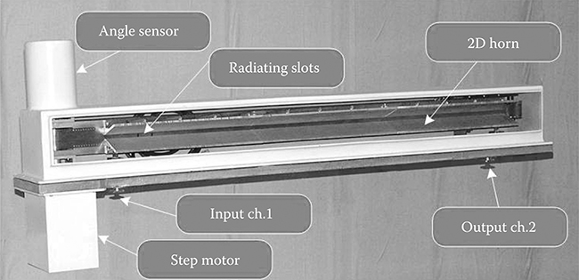
FIGURE 6.43
Lukin’s ground-based Ka-band noise SAR sliding slot antenna shown without the front radome. (Lukin, K.A. et al., “Ka-band ground-based noise waveform SAR,” Proc. 6th Int. Kharkov. Symp. Phys. Eng. Microwaves, Millimeter and Sub-millimeter Waves and Workshop on Terahertz Technologies-MSMW’2007, 1, 59-164, June 2007, © 2007 IEEE.)

Images

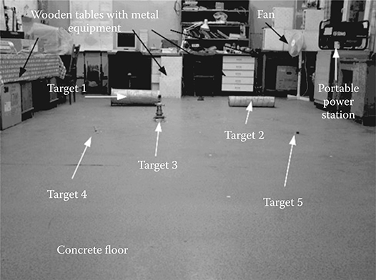
FIGURE 6.44
Photograph of the indoor trial scene observed by Lukin’s ground-based Ka-band noise SAR. (Courtesy of Professor K.A. Lukin.)

Images

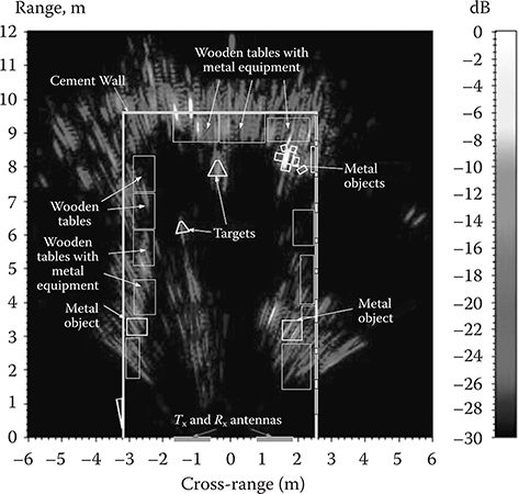
FIGURE 6.45
Processed image of the indoor scene in Figure 6.44. For reference, the locations of tables, walls, and objects are overlaid on the image. (Courtesy of Professor K.A. Lukin.)

Images

FIGURE 6.46
Photograph of the indoor trial scene observed by Lukin’s ground-based Ka-band noise SAR. (Courtesy of Professor K.A. Lukin.)

6.4.4 Future Potential Applications of Random Signal Radar

The combination of UWB technology and random signal radar can obtain both high-resolution target measurement and detection performance produced by an UWB waveform and also excellent EMC performance resulting from random signal modulation. This makes the UWB random signal radar very suitable for many applications in civil environments. Other suggested potential applications of UWB random signal radar include [49] automotive traffic monitoring, foreign object (such as debris) detection for railway and airport runway, concealed weapon detection through clothing for passenger security scanning, forward-looking radar for automated landing of aircrafts and automated docking of ships, etc.

Images

FIGURE 6.47
Processed image of the indoor scene in Figure 6.46: (a) Normal SAR image. (b) Interferogram. The two small targets are detected in the interferogram. (Courtesy of Professor K.A. Lukin.)

Images

FIGURE 6.48
Photograph of the St. Sophia cathedral bell tower and Lukin’s ground-based Ka-band noise waveform SAR system. (Lukin, K. et al., “Measurement of shifts in bell tower of Sophia cathedral using Ka-band noise waveform SAR,” Proc. 2nd. Int. Symp. Microwaves, Radar Remote Sensing, September 2008, © 2008 IEEE.)

Images

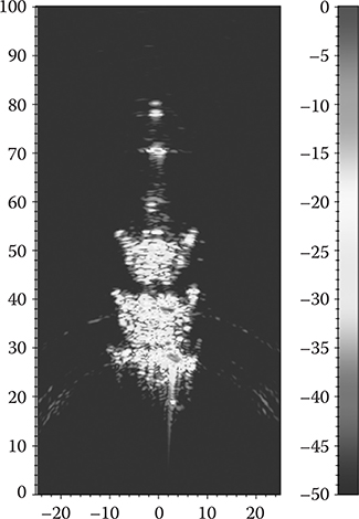
FIGURE 6.49
Processed image of the St. Sophia bell tower in Figure 6.48. (Courtesy of Professor K.A. Lukin.)

Images

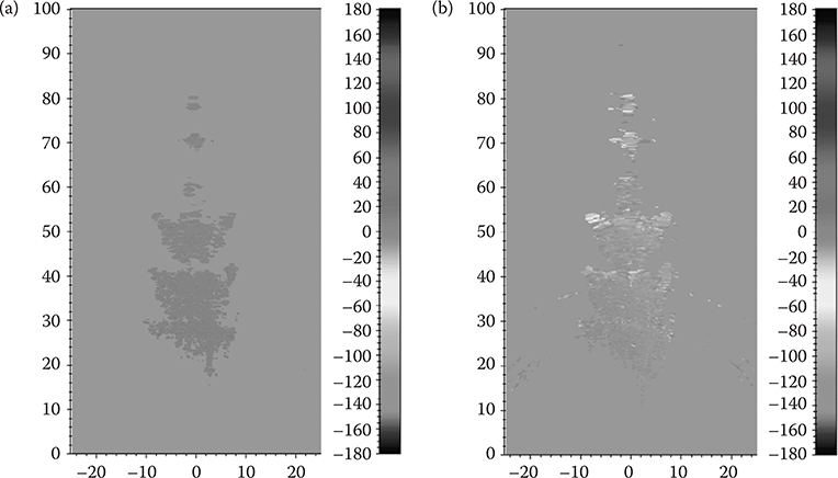
FIGURE 6.50
Differential interferogram of St. Sophia bell tower from data taken with an 1-h delay during (a) nighttime and (b) sunrise. (Courtesy of Professor K.A. Lukin.)

Images

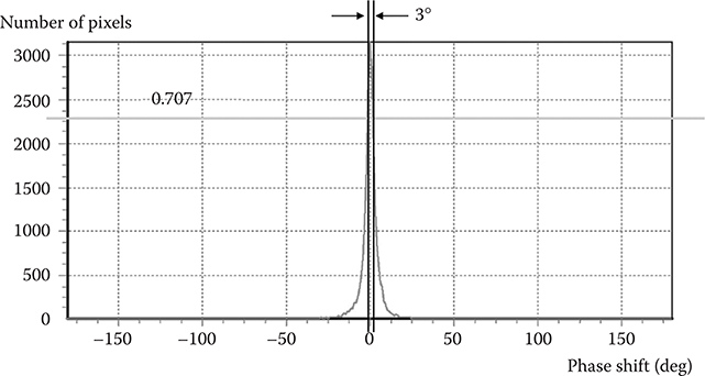
FIGURE 6.51
Histogram of the phase shift between two images obtained at night. (Lukin, K. et al., “Measurement of shifts in bell tower of Sophia cathedral using Ka-band noise waveform SAR,” Proc. 2nd. Int. Symp. Microwaves, Radar Remote Sensing, September 2008, © 2008 IEEE.)

Short-range surveillance for complex environments presents another attractive application scenario for civilian use, which has not received extensive explorations. In particular, the current counter-terrorist security applications urgently require sensitive all-weather, high-resolution, and reliable surveillance systems to cover a selected local complex area from a small factory to an international airport. Compared with the ultrasonic, laser, infrared, video sensors, or conventional radar systems, the UWB random signal radar presents the best candidate to satisfy all of the above-mentioned requirements.

First, short-range, wide-area, and high-resolution surveillance requires adopting the UWB waveform. In addition, the UWB waveform at low frequencies can also provide a wall or foliage penetration capability for the surveillance of a sensitive area. Next, civilian radars should have low cost and low energy consumption. A random signal radar working in CW mode can easily be implemented with very low cost and low energy consumption. Single high-power UWB radar systems may provide the required surveillance capability. However, multiple low-power systems can replace single, large expensive radar systems and perform more reliable surveillance. For some special application scenarios like the big warehouse or harbor area shown in Figure 6.52, there are many regularly or randomly distributed obstacles. For this case, a single high-power system cannot cover all the required areas. To assure complete coverage, a multistatic radar network of low-power radar sensors is required. Random signal modulation can provide a way to avoid interference among the multiple radar systems operating in the same area. Therefore, the configuration and signal processing of multistatic UWB random signal radar networks makes an attractive research topic, given the developing security requirements driven by current international counter-terrorist requirements.

Images

FIGURE 6.52
The noninterfering properties of the random signal radar can provide a solution to building a multistatic short-range surveillance system.

References

1. Van, L.B., Radar 101: Celebrating 101 years of development. Proc of the IEEE, Vol. 93, No. 4, pp 844-8846, April 2005.

2. Cherneyak, V.S., Immoreev, I.Y., and Vovshin, B.M., Radar in the Soviet Union and Russia: A brief historical outline. IEEE Aerosp Elect Syst Mag, Vol. 18, No. 12, pp 8-12, December 2003.

3. Bourret, R., A proposed technique for the improvement of range determination with noise radar. Proc of IRE, Vol. 45, No. 12, pp 1744-11744, December 1957.

4. Horton, B.M., Noise-modulated distance measuring systems. Proc of IRE, Vol. 49, No. 5, pp 821-8828, May 1959.

5. Grant, M.P., Cooper, G.R., and Kamal, A.K., A class of noise radar systems. Proc IEEE, Vol. 51, No. 7, pp 1060-11061, July 1963.

6. Copper, G.R. and McGillem, C.D., Random Signal Radar. Report TR EE-67-11, Purdue University, Lafayette, IN, June 1967.

7. McGillem, C.D., Copper, G.R., and Wiltaman, W.B., An experimental random signal radar. Proc Natl Electron Conf, Vol. 23, pp 409-4411, October 1967.

8. Cooper, G.R. and Purdy, R.J., Detection, Resolution and Accuracy in Random Signal radar. Report TR-EE 68-16, Purdue University, Lafayette, IN, August 1968.

9. Cooper, G.R. and Gassner, R.L. Analysis of a Wideband Random Signal Radar System. Report TR-EE 69-9, Purdue University, Lafayette, IN, August 1969.

10. Chadwick, R.B., Use of Random Signals to Study Distributed Radar Targets. Ph.D. Dissertation, Purdue University, Lafayette, IN, August 1970.

11. Chadwick, R.B. and Cooper, G.R., Measurement of distributed targets with random signal radar. IEEE Trans on Aerosp Elect Sys, Vol. 8, No. 6, pp 743-7750, November 1972.

12. Chadwick, R.B. and Cooper, G.R., A clutter reduction technique for random signal radars. IEEE Trans Aerosp Elect Sys, Vol. 10, No. 1, pp. 156-1160, January 1974.

13. Chadwick, R.B. and Cooper, G.R., Measurement of ocean wave heights with random signal radar. IEEE Trans Geosci Elect, Vol. 9, No. 4, pp 216-2221, October 1971.

14. Kaveh, M. and Cooper, G.R., Average ambiguity function for a randomly staggered pulse sequence. IEEE Trans Aerosp Elect Sys, Vol. 12, No. 3, pp 410-4413, May 1976.

15. Kaveh, M. and Cooper, G.R., Properties of randomly staggered pulsed random signal radar. Proc 1976 Elect Aerosp Sys Convention, Washington, D.C., pp 65A-65E, September 26-229, 1976.

16. Smit, J.A., Rudar—An experimental noise radar system. AGARD Conf Proc No. 66 Adv Radar Syst, North Atlantic Treaty Organization, pp 39.1-39.17, May 1970.

17. Forrest, J.R. and Meeson, J.P., Solid-state microwave noise radar. Elect Lett, Vol. 12, No. 15, pp 365-3366, July 1976.

18. Forrest, J.R. and Meason, J.P., Solid-state microwave noise radar. IEE Int Radar Conf, London, UK, pp 531-5534, October 1977.

19. Poirier, J.L., Quasi-monochromatic scattering and some possible radar applications. Radio Sci, Vol. 3, No. 9, pp. 881-8886, September 1968.

20. Schindler, J.K., Optimal spectrum filtering for the radar detection of targets in clutter. Phys Sci Res Papers. AD0853335. Air Force Cambridge Research Labs, January 1969.

21. Schindler, J.K. and Holt, F.S., Spectrum Analysis Radar. U.S. Patent 3745568, July 10, 1973.

22. Holt, F.S., Pierce, J.N., and Schindler J.K., Improved spectrum analysis noise radar systems. Phys Sci Res Papers. AD0768694. Air Force Cambridge Research Labs, April 1973.

23. Pierce, J.N. and Holt, S.F., Spectrum Analysis Radar System. U.S. Patent 3795912, May 1974.

24. Liu, G., Shi, X., and Lu, J., Random FM-CW radar and its ECCM. Proc 1986 Int Conf Radar, China, pp 155-1160, November 1986.

25. Liu, G., Shi, X., Lu, J., Yang, G., and Song, Y., Noise FM-CW radar system. Proc 1989 Int Symp Noise Clutter Rejection Radars Imaging Sensors, Japan, pp 578-5583, November 1989.

26. Liu, G., Shi, X., Lu, J., Yang, G., and Song, Y., Design of noise FM-CW radar and its implementation. IEE Proc—Part. F: Radar and Signal Process. Vol. 138, No. 5, pp 420-4426, September 1991.

27. Liu, G., Yang, G., and Zhu, D., A method obtain “HOLE” characteristic of spectral comparison type for noise radar. Proc 1987 Int Symp Electron Devices, Circuits Syst, India, pp 852-8853, December 1987.

28. Liu, G. and Gu, H., A comparison between random and pseudorandom binary phase-coded CW radar system. Proc 1991 Int Conf Radar, China, pp 390-3392, October 1991.

29. Liu, G. and Gu, H., Random binary phase coded CW radar system. Proc 1996 Int Conf Radar, China, pp 254-2258, October 1996.

30. Gu, H. and Liu, G., A new kind of radar—Random binary phase-coded CW radar. Proc 1997 Natl Radar Conf, Syracuse, New York, pp 202-2206, May 1997.

31. Wang, J. and Liu, G., Pulse random signal radar. Proc 1996 Int Conf Radar, China, pp 523-5526, October 1996.

32. Liu, G., Gu, H., Zhu, X., and Su W., The present and the future of random signal radars. IEEE Aerospace Elect Syst Mag, Vol. 12, No. 10, pp 35-340, October 1997.

33. Liu, G., Gu, H., and Su, W., The development of random signal radar. IEEE Trans Aerospace Elect Sys, Vol. 35, No. 3, pp 770-7777, July 1999.

34. Gu, H. and Su, W., A new quasi-continues wave radar. Proc 9th Chinese Natl Radar Symp, China, pp 23-226, April 2004 (in Chinese).

35. Narayanan, R.M., Hoffmeyer, P.D., and Curtis, J.O., Design, performance, and applications of a coherent ultra-wideband random noise radar. Opt Eng, Vol. 37, No. 6, pp 1855-11869, June 1998.

36. Xu, Y., Narayanan, R.M., Xu, X., and Curtis, J.O., Polarimetric processing of coherent random noise radar data for buried object detection. IEEE Trans Geosci Rem Sens, Vol. 39, No. 3, pp 467-4478, March 2001.

37. Xu, X. and Narayanan, R.M., FOPEN SAR imaging using UWB step-frequency and random noise waveforms. IEEE Trans Aerosp Elect Sys, Vol. 37, No. 4, pp 1287-11300, October 2001.

38. Narayanan, R.M. and Kumru, C., Implementation of fully polarimetric random noise radar. IEEE Antennas Wireless Propagat Lett, Vol. 4, pp 125-1128, 2005.

39. Narayanan, R.M., Xu, X., and Henning, J.A., Radar penetration imaging using ultra-wideband (UWB) random noise waveforms. IEE Proc-Radar, Sonar Navigation, Vol. 151, No. 3, pp 143-1148, June 2004.

40. Garmatyuk, D.S. and Narayanan, R.M., Ultra-wideband continuous-wave random noise arc-SAR. IEEE Trans Geosci Remote Sens, Vol. 40, No. 12, pp 2543-22552, December 2002.

41. Bell, D.C. and Narayanan, R.M., ISAR imaging using coherent random noise radar techniques. Proc SPIE Conf Radar Process, Technol Appl III, San Diego, CA, Vol. 3462, pp 284-2295, July 1998.

42. Bell, D.C. and Narayanan, R.M., Inverse synthetic aperture radar imaging using a coherent ultra-wideband random noise radar system. Opt Eng, Vol. 40, No. 11, pp 2612-22622, November 2001.

43. Zhang, Y. and Narayanan, R.M., Design considerations for a real-time random-noise tracking radar. IEEE Trans Aerospace Elect Sys, Vol. 40, No. 2, pp 434-4445, April 2004.

44. Xu, X. and Narayanan, R.M., Range sidelobe suppression technique for coherent ultra-wideband random noise radar imaging. IEEE Trans Antennas Propagat, Vol. 49, No. 12, pp 1836-11842, December 2001.

45. Narayanan, R.M. and Dawood, M., Doppler estimation using a coherent ultrawide-band random noise radar. IEEE Trans Antennas Propagat., Vol. 48, No. 6, pp 868-8878, June 2000.

46. Li, Z. and Narayanan, R.M., Doppler visibility of coherent ultrawideband random noise radar systems. IEEE Trans Aerospace Elect Sys, Vol. 42, No. 3, pp 904-9916, July 2006.

47. Bell, D.C. and Narayanan, R.M., Theoretical aspects of radar imaging using stochastic waveforms. IEEE Trans Signal Process, Vol. 49, No. 2, pp 394-3400, February 2001.

48. Zhang, Y. and Narayanan, R.M., Monopulse radar based on spatiotemporal correlation of stochastic signals. IEEE Trans Aerospace Elect Sys, Vol. 42, No. 1, pp 160-1173, January 2006.

49. Lukin, K.A., Noise radar technology for short range application. Proc 5th Int Conf Exhibition Radar Sys—RADAR’1999, France, May 1999.

50. Lukin, K.A., Millimeter wave noise radar applications: Theory and experiment. Proc 4th Int Kharkov Symp Phys Eng Millimeter and Sub-millimeter Waves, Vol. 1, pp 68-673, June 2001.

51. Tarchi, D., Lukin, K., Leva, D., Fortuni, J., Mogila, A., Vyplavin, P., and Sieber, A., Implementation of noise radar technology in ground based SAR for short range applications. Proc 6th Int Kharkov Symp Phys Eng Microwaves, Millimeter and Sub-millimeter Waves and Workshop on Terahertz Technologies—MSMW’2007, Vol. 1, pp 442-4444, June 2007.

52. Lukin, K.A., Mogyla, A.A., Vyplavin, P.L., Palamarchuk, V.P., Zemlyaniy, O.V., Shiyan, Y., Zaets, N.K., Skresanov, V.N., Shubniy, A.I., Glamazdin, V., Natarov, M.P., and Nechayev, O.G., Ka-band ground-based noise waveform SAR. Proc 6th Int Kharkov Symp Phys Eng of Microwaves, Millimeter and Sub-millimeter Waves and Workshop on Terahertz Technologies—MSMW’2007, Vol. 1, pp 159-1164, June 2007.

53. Lukin, K.A., Mogyla, A.A., Palamarchuk, V.P., Vyplavin, P.L., Zemlyaniy, O.V., Shiyan, Y.A., and Zaets, M., Ka-band bistatic ground-based noise waveform SAR for short-range applications. IET Radar, Sonar Navigation, Vol. 2, No. 4, pp 233-2243, August 2008.

54. Lukin, K., Mogyla, A., Palamarchuk, V., Vyplavin, P., Kozhan, E., and Lukin, S., Monitoring of St. Sophia cathedral interior using Ka-band ground based noise waveform SAR. Proc 2009 European Radar Conf—EuRAD’2009, Italy, pp 215-2217, September-October 2009.

55. Lukin, K., Mogyla, A., Palamarchuk, V., Vyplavin, P. and Kozhan, E., Measurement of shifts in bell tower of Sophia cathedral using Ka-band noise waveform SAR. Proc 2nd Int Symp Microwaves, Radar Remote Sensing, Ukraine, September 2008.

56. Lukin, K.A., Noise radar with correlation receiver as the basis of car collision avoidance system. Proc 25th European Microwave Conf, Vol. 1, Italy, pp 506-5507, October 1995.

57. Lukin, K.A., Mogyla, A.A., Alexandrov, Y.A., Zemlyaniy, O.V., Lukina, T., and Shiyan, Y., W-band noise radar sensor for car collision warning systems. Proc 4th Int Kharkov Symp Phys Eng Millimeter and Sub-millimeter Waves, Vol. 2, pp 870-8872, June 2001.

58. Lukin, K.A., Kulyk, V., and Zemlyaniy, O.V., Chaos generators for noise radar. In I.N. Visarath et al. (eds.), Applications of Nonlinear Dynamics: Model and Design of Complex Systems, Springer, Berlin, 2009.

59. Walton, E.K., Fillimon, V., and Gunawan, S., ISAR imaging using UWB noise radar. Proc 18th Ann Meeting Symp Ant Measurement Technol Assoc, Seattle, WA, pp 167-1171, September-October 1996.

60. Walton, E.K., Theron, I.P., Gunawan, S., and Cai, L., Moving vehicle range profiles measured using a noise radar. Proc 1997 IEEE. Ant Propagat Soc Int Symp, Vol. 4, pp 2597-22600, July 1997.

61. Theron, I.P., Walton, E.K., Gunawan, S., and Cai, L., Ultrawide-band noise radar in the VHF/UHF band. IEEE Trans Ant Propagat, Vol. 47, No. 6, pp 1080-11084, June 1999.

62. Theron, I.P., Walton, E.K., and Gunawan, S., Compact range radar cross-section measurements using a noise radar. IEEE Trans Ant Propagat, Vol. 46, No. 9, pp 1285-11288, September 1998.

63. Stephan, R. and Loele, H., Theoretical and practical characterization of a broadband random noise radar. Proc IEEE 2000 Int Microwave Symp, Boston, MA, Vol. 1-3, pp 1555-11558, June 2000.

64. Axelsson, S.R.J., Noise radar using random phase and frequency modulation. IEEE Trans Geosci Remote Sens, Vol. 42, No. 11, pp 2370-22384, November 2004.

65. Special Issue on Signal Processing in Noise Radar Technology. IET Radar, Sonar Navigation, Vol. 2, No. 4, August 2008.

66. Xu, X. and Narayanan, R.M., Impact of different correlation receiving techniques on the imaging performance of UWB random noise radar. Proc 2003 IEEE Int Geosci Remote Sensing Symp— IGARSS’2003, France, Vol. 7, pp 4525-44527, July 2003.

67. Axelsson, S.R.J., Noise radar for range/Doppler processing and digital beamforming using low-bit ADC. IEEE Trans Geosci Remote Sensing, Vol. 41, No. 12, pp 2703-22720, December 2003.

68. Sun, H., Lu, Y., and Liu, G., Ultra-wideband technology and random signal radar: An ideal combination. IEEE Aerospace Elect Sys Mag, Vol. 18, No. 11, pp 3-7, November 2003.

69. Khan, R.H. and Mitchell, D.K., Waveform analysis for high-frequency FMICW radar. IEE Proc F Radar Signal Process, Vol. 138, No. 5, pp 411-4419, October 1991.

70. Gu, H., Li, X., Shang, W., Su, W., and Liu, G., A new approach of periodic square-wave interruption to solution of the leakage of CW radar. Acta Electron Sinica, Vol. 26, No. 12, pp 7-11, December 1998 (in Chinese).

71. Hussain, M.G.M., Principles of high-resolution radar based on nonsinusoidal waves—Part 1: Signal representation and pulse compression. IEEE Trans Electromag Compatibil, Vol. 31, No. 4, pp 359-3368, November 1989.

72. Liu, G., Gu, H., Su, W., Sun, H., and Zhang, J., Random signal radar—A winner in both the military and civilian operating environments. IEEE Trans Aerospace Elect Sys, Vol. 39, No. 2, pp 489-4498, April 2003.

73. Mogila, A.A., Lukin, K.A., Kovalenko, N.P., and Kovalenko, R.P., Ka-band noise SAR simulation. Proc 4th Int Kharkov Symposium Phys Eng Millimeter and Sub-millimeter Waves, Kharkov, Ukraine, Vol. 1, pp 441-4443, June 2001.

74. Schleher, D.C., Low probability of intercept radar. Proc 1985 IEEE Int Radar Conf, Arlington, VA, pp 346-3349, May 1985.

75. Thayaparan, T., Dakovic, M., and Stankovic, L., Mutual interference and low probability of interception capabilities of noise radar. IET Radar Sonar Navigation, Vol. 2, No. 4, pp 294-2305, August 2008.

76. Garmatyuk, D.S. and Narayanan, R.M., ECCM capabilities of an ultrawideband bandlimited random noise imaging radar. IEEE Trans Aerosp Elect Sys, Vol. 38, No. 4, pp 1243-11255, October 2002.

77. Detlefsen, J., Schmidhammer, E., and Troll, T., Collision warning radar using PN-code-modulation and wavefront reconstruction. Proc 1998 Int Radar Symp, Munich, Germany, pp 363-3370, September 1998.

78. Kajiwara, A., Vehicular stepped-FM coded radar for collision avoidance. Proc 1998 IEEE Int Conf Vehicular Technol, Ottawa, Canada, pp 2085-22089, May 1998.

79. Zhang, J., Liu, G., Gu, H., and Su, W., A novel transmit signal based on high range-resolution concept for FLAR or AICC system application. Proc CIE 2001 Int Conf Radar, China, pp 81-884, October 2001.

80. Liu, G., Gu, H., Zhu, X., Sun, Y., Sun, G., and Su, W., A contrast experiment of ECCM of random to pseudorandom binary phase coded CW radar. Proc IEEE 1996 Int Conf Signal Process, China, pp 1621-11624, October 1996.

81. Adrian, D.J., Autocorrelation Type Spectral Comparison Fuze System. U.S. Patent 3906493, September 16, 1975.

82. Adrian, D.J., FM Autocorrelation Fuze System. U.S. Patent 4232314, November 4, 1980.

83. Whitely, T.B. and Adrian, D.J., Random FM Autocorrelation Fuze System. U.S. Patent 4220952, September 2, 1980.

84. Liu, G., Shi, X., and Lu, J., Random FM-CW Radar Fuze System. Chinese Invention Patent 85105878, August 7, 1987.

..................Content has been hidden....................

You can't read the all page of ebook, please click here login for view all page.

Table of Contents for 6 Ultrawideband and Random Signal Radar

Create new playlist

Sign In

Sign Up

Table of Contents for
6 Ultrawideband and Random Signal Radar