8 UWB Pulse Backscattering from Objects Located near Uniform Half-Space

This chapter is devoted to the theory of backscattering of ultrawideband (UWB) pulse signal from perfect electrically conducting (PEC) large objects. The analysis considers targets located near the boundary of uniform half-space with both real and complex electrical parameters. The approach uses a high-frequency (physical optics approach) approximation of pulse (transient) wavefront characteristics to calculate the UWB response of the object by convolution transformation. The calculation method uses developed field integral representations and the high-frequency approximation of a (PEC) object pulse characteristic (PC) in a general bistatic case for oblique incidence. This also deals with the problem of UWB signal scattering from the half-space, representing a layered uniform medium with arbitrary layers of complex permeabilities. These analytical methods have many potential applications for estimating UWB signal responses from large targets.

8.2 Superwideband Signal Scattering in the Layered Half-Space with Parameters of Ground

8.2.1 Objectives

The solution of many electrodynamic-medium distance sounding problems and radar problems requires finding the solution of the problem of UWB signal scattering from the half-space. The half-space represents a layered uniform medium with arbitrary complex electrodynamic parameters of layers near an electrically large target, which is much larger than the physical pulse length cτ, where τ is the pulse duration. Determining the target response requires obtaining the smoothed PC from the Gaussian videopulse for the multi-layered earth surface. R. W. P. King [1] solved this problem for the particular case of normal incidence of the Gaussian videopulse on the boundary of the uniform half-space.

L. M. Brekhovskikh [2] researched this problem for the arbitrary incidence of the plane-polarized pulsed wave on the half-space mentioned above. In contrast, the methods developed in this chapter provide a general solution to the problem and allow to calculate the pulse fields in all points of the sounding half-space.

The received results can be physically justified if one considers the approximately calculated reflected or refracted pulse signal as the response of an object to the components of multiple finite front plane waves, which is codirected with the scattering pulse wave distribution.

8.2.2 Problem Solution Method

We will consider only the case of the pulse physical size cτ ≪ target size. Our examination assumes a scattering problem of the sounding UWB signal on the layered uniform half-space as shown in Figure 8.1:

$\begin{array}{l} \begin{matrix} {\vec{\begin{matrix} ℰ \end{matrix}}}^{0} ({\vec{R}}^{0}, t) = {\vec{p}}^{0} Q (t + {\vec{R}}^{0} \vec{x}), \\ {\vec{ℋ}}^{0} ({\vec{R}}^{0}, t) = \sqrt{\frac{ε_{0}}{μ_{0}}} [{\vec{p}}^{0} \times {\vec{R}}^{0}] Q (t + {\vec{R}}^{0} \vec{x}), \end{matrix} \\ Q (t + {\vec{R}}^{0} \vec{x}) = \frac{1}{\sqrt{π} τ_{u}} exp [- \frac{{(t + {\vec{R}}^{0} \vec{x})}^{2}}{τ_{u}^{2}}] - \frac{1}{1.5 \sqrt{π} τ_{u}} exp [- \frac{{(t + {\vec{R}}^{0} \vec{x})}^{2}}{{(1.5 τ_{u})}^{2}}] . \end{array} (8.1)$

Here - ${\vec{R}}^{0}$ = (sin θ,0, cos θ) is the unit normal to the incident wavefront, ${\vec{p}}^{0} = (p_{1}^{0}, p_{2}^{0}, p_{3}^{0})$ is the unit polarization vector, and τ_u = cτ is the pulse physical length, when τ is the pulse duration in seconds. The half-space is divided into areas G_i (i = 0, 1, ...s, m) with complex permittivities ε_i and permeabilities μ_i, correspondingly. The vectors ${\vec{ℰ}}^{0}$ and ${\vec{ℋ}}^{0}$ characterize electrical and magnetic components of the sounding signal, and Q(t) is the time-dependence of this signal.

Images

FIGURE 8.1
The sounding medium model showing the characteristics of layers at different depths.

Taking into account that the signal of Equation 8.1 is the Fourier-original for the stationary plane wave, so that

$\begin{matrix} \begin{matrix} {\vec{E}}^{0} (\vec{x}) = {\vec{p}}^{0} exp (- j k_{0} ({\vec{R}}^{0} \vec{x})), \\ {\vec{H}}^{0} (\vec{x}) = \sqrt{\frac{ε_{0}}{μ_{0}}} ({\vec{p}}^{0} \times {\vec{R}}^{0}) exp (- j k_{0} ({\vec{R}}^{0} \vec{x})), \end{matrix} \end{matrix} (8.2)$

the response to the signal of Equation 8.1 ${\vec{ℰ}}^{0} (\vec{x}, t)$ , ${\vec{ℋ}}^{0} (\vec{x}, t)$ can be received in the form of a reverse Fourier transformation from the product of spectral density of the pulse signal and the frequency characteristic of the medium. For example,

$\vec{ℰ} (\vec{x}, t) = (2 π)^{1} \int_{- \infty}^{\infty} \vec{E} (\vec{x}) S ({\vec{R}}^{0}, k) \exp (- j k t) d k, (8.3)$

where

$S ({\vec{R}}^{0}, k) = \exp [- \frac{(τ_{u} k)^{2}}{4}] - exp [- \frac{(1.5 τ_{u} k)^{2}}{4}],$

and $\vec{E} (\vec{x})$ is the frequency characteristic of the medium when a field is generated in space by incident monochromatic plane wave of Equation 8.2.

Therefore, to obtain the transient field of Equation 8.3, it is necessary to calculate the frequency characteristic of the medium $\vec{E} (\vec{x})$ in any of G_i(i = 0,1, . . . ,m) areas.

In region G₀ of Figure 8.1, we will calculate the required (reflected) field in the following form:

$\begin{array}{l} \vec{E} (\vec{x}) = {\vec{p}}^{1} \exp (- j k_{0} ({\vec{R}}^{1} \vec{x})), \\ \vec{H} (\vec{x}) = \sqrt{\frac{ε_{0}}{μ_{0}}} ({\vec{p}}^{1} \times {\vec{R}}^{1}) \exp (- j k_{0} ({\vec{R}}^{1} \vec{x})), \end{array} (8.4)$

where ${\vec{R}}^{1} = (- sin θ, 0, cos θ)$ , and the vector ${\vec{p}}^{1}$ is to be determined.

We will calculate the field that passed through the layered structure in the half-space G_m in the same form as the plane wave:

$\begin{array}{l} \vec{E} (\vec{x}) = {\vec{p}}^{m} \exp (- {j k}_{m} ({\vec{R}}^{m} \vec{x})), \\ \vec{H} (\vec{x}) = \sqrt{\frac{ε_{m}}{μ_{m}}} ({\vec{p}}^{m} \times {\vec{R}}^{m}) \exp (- j k_{m} ({\vec{R}}^{m} \vec{x})) . \end{array} (8.5)$

Here $k_{m} = k_{0} \sqrt{ε_{m}^{'} μ_{m}^{'}}, ε_{m}^{'} = ε_{m} / ε_{0}, μ_{m}^{'} = μ_{m} / μ_{0}, k_{0} = ω \sqrt{ε_{0}^{'} μ_{0}^{'}, ω}$ is the frequency of the incident plane wave ${\vec{R}}^{m} = (- sin θ_{m}, 0, - cos θ_{m})$ . Vector ${\vec{p}}^{m}$ and value θ_m (both complex in the general case) are to be determined. In this case, the orthogonal conditions must exist such that

$({\vec{p}}^{0} {\vec{R}}^{0}) = ({\vec{p}}^{1} {\vec{R}}^{1}) = ({\vec{p}}^{m} {\vec{R}}^{m}) = 0. (8.6)$

To find the field inside the layer G_i (i = 1, ..., m−1), we use Maxwell equations:

${\begin{cases} j k_{0} μ_{i}^{'} \vec{H} = \frac{1}{W_{0}} (\vec{\nabla} \times \vec{E}), \\ - j k_{0} ε_{i}^{'} \vec{E} = W_{0} (\vec{\nabla} \times \vec{H}), \end{cases} (8.7)$

where

$W_{0} = \sqrt{\frac{ε_{0}}{μ_{0}}}$

is the wave resistance and

$\vec{\nabla} = \vec{i} \frac{\partial}{\partial x} + \vec{j} \frac{\partial}{\partial y} + \vec{k} \frac{\partial}{\partial z}$

is the Hamilton operator.

We can introduce the designations ${\vec{A}}_{⊥} = {\vec{e}}_{z} \vec{A}, {\vec{A}}_{T} = {\vec{A}}_{⊥} {\vec{e}}_{z}$ , and ${\vec{A}}_{z} = \vec{A} {\vec{e}}_{z}$ , where ${\vec{e}}_{x}, {\vec{e}}_{y}$ , and ${\vec{e}}_{z}$ are the unit vectors of Cartesian frame of reference.

From the system of Equations 8.7, the relations linking the tangential and normal (in relation to the media boundary) components of vectors $\vec{E}$ and $\vec{H}$ can be obtained:

$j k_{0} μ_{i}^{'} W_{0} {\vec{H}}_{⊥} = - \frac{\partial {\vec{E}}_{T}}{\partial z} + {\vec{e}}_{x} \frac{\partial E_{z}}{\partial x}, (8.8)$

$j k_{0} ε_{i}^{'} \frac{1}{W_{0}} {\vec{E}}_{T} = - \frac{\partial {\vec{H}}_{⊥}}{\partial z} + {\vec{e}}_{y} \frac{\partial H_{z}}{\partial x}, (8.9)$

$j k_{0} μ_{i}^{'} W_{0} H_{z} = {\vec{e}}_{y} \frac{\partial {\vec{E}}_{T}}{\partial x}, (8.10)$

$j k_{0} ε_{i}^{'} \frac{1}{W_{0}} E_{z} = {\vec{e}}_{x} \frac{\partial {\vec{H}}_{⊥}}{\partial x} . (8.11)$

Let us search the field in layer G_i (i = 0, 1, ..., m) in the form

$\begin{array}{l} \vec{E} (\vec{x}) = \tilde{\vec{E}} (z) \exp (j k_{0} x \sin θ), \\ \begin{matrix} \begin{matrix} \vec{H} (\vec{x}) = = \tilde{\vec{H}} (z) exp ({j k}_{0} x sin θ), \end{matrix} & where (0 < z < δ_{m - 1}) . \end{matrix} \end{array} (8.12)$

Then from Equations 8.8 through 8.11, the following relations can be obtained:

${\tilde{E}}_{z} = \frac{W_{0}}{ε_{i}^{'}} \sin θ ({\vec{e}}_{x} \cdot {\tilde{\vec{H}}}_{⊥}), (8.13)$

$\frac{1}{j k_{0} μ_{i}^{'} W_{0}} \frac{\partial {\tilde{\vec{E}}}_{T}}{\partial z} = - {\tilde{\vec{H}}}_{⊥} + \frac{\sin^{2} θ}{ε_{i}^{'} μ_{i}^{'}} {\vec{e}}_{x} ({\vec{e}}_{x} \cdot {\tilde{\vec{H}}}_{⊥}), (8.14)$

${\tilde{H}}_{z} = \frac{\sin θ}{μ_{i}^{'} W_{0}} ({\vec{e}}_{y} \cdot {\tilde{\vec{E}}}_{T}), (8.15)$

$\frac{W_{0}}{j k_{0} ε_{i}^{'}} \frac{\partial \tilde{\vec{H}}}{\partial z} = - {\tilde{\vec{E}}}_{T} + \frac{\sin^{2} θ}{ε_{i}^{'} μ_{i}^{'}} {\vec{e}}_{y} ({\vec{e}}_{y} \cdot {\tilde{\vec{E}}}_{T}) . (8.16)$

The system of linear Equations 8.8 through 8.16 is decomposed into two systems:

$\frac{\partial}{\partial z} [\begin{matrix} U_{1} \\ V_{1} \end{matrix}] = A_{1}^{(i)} [\begin{matrix} U_{1} \\ V_{1} \end{matrix}], (8.17)$

$\frac{\partial}{\partial z} [\begin{matrix} U_{2} \\ V_{2} \end{matrix}] = A_{2}^{(i)} [\begin{matrix} U_{2} \\ V_{2} \end{matrix}], (8.18)$

where

$\begin{array}{l} \vec{U} (z) = U_{1} (z) {\vec{e}}_{x} + U_{2} (z) {\vec{e}}_{y} = {\tilde{\vec{E}}}_{T} (z), \\ \vec{V} (z) = V_{1} (z) {\vec{e}}_{x} + V_{2} (z) {\vec{e}}_{y} = {\tilde{\vec{H}}}_{⊥} (z), \end{array}$

and

$A_{1}^{(i)} = [\begin{matrix} 0 & \frac{W_{0}}{j k_{0} ϵ_{i}^{'}} γ_{i}^{2} \\ - \frac{j k_{0} ϵ_{i}^{'}}{W_{0}} & 0 \end{matrix}], A_{2}^{(i)} = [\begin{matrix} 0 & - j k_{0} μ_{i}^{'} W_{0} \\ - \frac{γ_{i}^{2}}{j k_{0} μ_{i}^{'} W_{0}} & 0 \end{matrix}], γ_{i}^{2} = k_{0}^{2} (ϵ_{i}^{'} μ_{i}^{'} - {sin}^{2} θ) .$

Since $A_{1}^{{(i)}^{2}} = A_{2}^{{(i)}^{2}} = - γ_{i}^{2} I$ (I is the unit matrix), we get

$A_{k}^{(i)^{2 m}} = (- 1)^{m} γ_{i}^{2 m} I; A_{k}^{{(i)}^{2 m + 1}} = (- 1)^{m} γ_{i}^{2 m} A_{k}^{(i)}, (m = 0, 1, 2, ...; k = 1, 2, . . .),$

and the matrix exponential

$\exp (z A_{k}^{(i)}) = I \cos (γ_{i} z) + A_{k}^{(i)} \frac{\sin (γ_{i} z)}{γ_{i}}, (k = 1, 2, . . .) . (8.19)$

Taking into account the equality in Equation 8.19, the solution of the system shown in Equations 8.17 and 8.18 can be represented as

$\begin{matrix} (\begin{matrix} U_{k} (z) \\ V_{k} (z) \end{matrix}) = [I cos (γ_{i} (z - δ_{i - 1})) + A_{k}^{(i)} \frac{sin (γ_{i} (z - δ_{i - 1}))}{γ_{i}}] B_{k}^{(i - 1)} (\begin{matrix} U_{k} (0) \\ V_{k} (0) \end{matrix}), \\ where (δ_{i 1} < z < δ_{i} and k = 1, 2...) . \end{matrix} (8.20)$

where the matrix operator

$B_{k}^{(i - 1)} = Π_{l = 1}^{i - 1} [I cos (γ_{l} (δ_{l} - δ_{l - 1})) + A_{k}^{(l)} \frac{sin (γ_{l} (δ_{l} - δ_{l - 1}))}{γ_{l}}] .$

In particular,

$(\begin{matrix} U_{k} (δ_{m - 1}) \\ V_{k} (δ_{m - 1}) \end{matrix}) = B_{k}^{(m - 1)} (\begin{matrix} U_{k} (0) \\ V_{k} (0) \end{matrix}) . (8.21)$

In Equations 8.20 and 8.21, the values U_k (0) and V_k (0) are unknown and must be determined by boundary conditions.

From the conditions of the kind ${\vec{E}}_{T}^{+} = {\vec{E}}_{T}^{-}$ and ${\vec{H}}_{T}^{+} = {\vec{H}}_{T}^{-}$ on the planes z = 0 and z = δ_{m − 1} taking into account Equation 8.12, it is possible to obtain the relation between the values $\vec{U}$ and $\vec{V}$ when z = 0 (i.e., on the top boundary of the area G₁)

$\vec{V} \cos θ - \frac{1}{W_{0}} [\vec{U} - \sin^{2} θ \cdot {\vec{e}}_{y} ({\vec{e}}_{y} \cdot \vec{U})] = 2 \cos θ ({\vec{e}}_{z} \times (\vec{p} \times {\vec{R}}^{0})) (8.22)$

as well as the relation between the vector function $\vec{U}$ and $\vec{V}$ when z = δ_m−1 (i.e., on the bottom boundary of the area G_m−1):

$\sqrt{\frac{ε_{m}^{'}}{μ_{m}^{'}}} \vec{V} \cdot \cos θ_{m} = - \vec{U} + \sin^{2} θ_{m} \cdot {\vec{e}}_{y} (\vec{U} \cdot {\vec{e}}_{y}) (8.23)$

and

$\sin θ_{m} = \frac{\sin θ}{\sqrt{ε_{m}^{'} μ_{m}^{'}}} . (8.24)$

Vector equalities of Equations 8.22 and 8.23 are decomposed into two scalar systems of boundary conditions corresponding to differential systems 8.17 and 8.18:

${\begin{matrix} \sqrt{\frac{μ_{0}}{ε_{0}}} V_{1} (0) \cos θ - U_{1} (0) = - 2 p_{1}^{0} \\ \sqrt{\frac{μ_{m}}{ε_{m}}} V_{1} (δ_{m - 1}) \cos θ_{m} + U_{1} (δ_{m - 1}) = 0 \end{matrix}, (8.25)$

${\begin{matrix} \sqrt{\frac{μ_{0}}{ε_{0}}} V_{2} (0) - U_{2} (0) \cos θ = - 2 p_{2}^{0} \cos θ \\ \sqrt{\frac{μ_{m}}{ε_{m}}} V_{2} (δ_{m - 1}) + U_{2} (δ_{m - 1}) \cos θ_{m} = 0 \end{matrix} . (8.26)$

The linear algebraic system of Equation 8.25 with the system of Equation 8.21 when k = 1 and the system of Equation 8.26 along with the system of Equation 8.21 when k = 2 allow determining the vectors ( ${\vec{U}}_{1} (0)$ , ${\vec{V}}_{1} (0)$ ) and ( ${\vec{U}}_{2} (0)$ , ${\vec{V}}_{2} (0)$ ), respectively. When the mentioned vectors have been determined, it is possible to calculate the formula in Equation 8.20, thus to find values ${\tilde{\vec{E}}}_{T} (z)$ , ${\tilde{\vec{H}}}_{T} (z)$ for any 0〈z〈δ_m−1, and then to calculate the field $\vec{E} (\vec{x})$ , $\vec{H} (\vec{x})$ using the Equation 8.12.

The vector components ${\vec{p}}^{m} = {\vec{p}}_{T}^{m} + {\vec{e}}_{z} \cdot p_{z}^{m}$ necessary for finding the field in the area G_m are determined by the following formulas:

${\vec{p}}_{T}^{m} = \vec{U} (δ_{m - 1}) \exp (- j k_{m} δ_{m - 1} \cos θ_{m}), (8.27)$

${\vec{p}}_{z}^{m} = - \tan θ_{m} ({\vec{p}}_{T}^{m} {\vec{e}}_{x}) . (8.28)$

To meet the condition of field reduction when z → ∞ the branch of root for calculation

$\cos θ_{m} = \sqrt{1 - \sin^{2} θ_{m}}$

should be determined from the condition

$I m (\sqrt{ε_{m}^{'} μ_{m}^{'}} \cos θ_{m}) > 0 .$

Vector components ${\vec{p}}_{1} = {\vec{p}}_{T}^{1} + {\vec{e}}_{z} {\vec{p}}_{z}^{1}$ are determined from the boundary conditions at z = 0 using the formulas:

${\vec{p}}_{T}^{1} = \vec{U} (0) - {\vec{p}}_{T}, (8.29)$

${\vec{p}}_{z}^{1} = \tan θ ({\vec{p}}_{T}^{1} {\vec{e}}_{x}) . (8.30)$

Thus, having determined the required frequency characteristic $\vec{E} (\vec{x})$ of the sounding medium, we can calculate the pulse UWB signal $\vec{ℰ} (\vec{x}, t)$ by means of the equality in Equation 8.3 in any of G_i(i = 0, 1, ... , m) areas.

A series of numerical calculations illustrate the method described above.

8.2.3 Results of Numerical Calculations

We chose models of sounding medium for numerical calculation. The models represent layered uniform structures with the following parameters shown in Table 8.1.

We selected a horizontal polarization UWB probing signal as shown in Equation 8.1 with 1 μs, 0.5 μs, and 1 and 10-ns duration (for level −6dB from peak value).

We did the calculations when probing the second model at the angle of 20° by the signal with 1-μs duration on different layers. Table 8.2 summarizes the test conditions shown in Figures 8.2 through 8.5. In Figures 8.2 through 8.6, h(t) corresponds to horizontal projection of $\vec{ℰ} (\vec{x}, t)$ , and v(t) corresponds to vertical projection of $\vec{ℰ} (\vec{x}, t)$ .

The qualitative view of the plots obtained in all cases of passing of the UWB signal in a material medium (Figures 8.2 through 8.5) has the same tendency as that in the plots obtained at normal (to ground) incidence of the UWB videopulse in the case of half-space [1].

Figure 8.3 shows how the response amplitude in the material medium decreases as the incident angle increases, that is, the ground surface reflects more of the pulse energy with the increasing incident angle. The field strength attenuation occurs faster in wet ground than in dry ground (see Figures 8.2 and 8.3a), and more severe attenuation occurs at high frequencies. The ground–air boundary reflects better the lower frequencies of the pulse spectrum. With the increasing depth, we observe the maximum response shift and amplitude reduction. Figure 8.2d describes the moment when the response changes its form.

TABLE 8.1
Characteristics of Sounding Medium Model

Medium Model	1	2	3
Layer 1	Dry soil (2.3 m): $ε_{r}^{'} = 7$ , σ = 10^-3 S/m, μ′ = 1	Wet soil (2.3 m): $ε_{r}^{'} = 30$ , σ = 3 × 10^-2 S/m, μ′ = 1	Granite (0.2 m): $ε_{r}^{'} = 11$ , σ = 10^-6 S/m, μ′ = 1
Layer 2	Dry sandstone (4.7 m): $ε_{r}^{'} = 9$ , σ = 10^-6 S/m, μ′ = 1	Wet sandstone (4.7 m): $ε_{r}^{'} = 9$ , σ = 10^-2 S/m, μ′ = 1	Air (0, 1, or 3 m): $ε_{r}^{'} = 1$ , μ′ = 1
Layer 3	Clay: $ε_{r}^{'} = 10$ , σ = 10^-5 S/m, μ′ = 1	Wet clay: $ε_{r}^{'} = 10$ , σ = 10^-3 S/m, μ′ = 1	Clay: $ε_{r}^{'} = 10$ , σ = 10^-5 S/m, μ′ = 1

TABLE 8.2
Summary of Radar Probe Test Conditions

Response Results	Model	Depth (m)	Incident Angle (degrees)	Pulse Duration	Polarization
Figure 8.2	2	1.1, 2.1, 4.8, 30	20	1 μs	Horizontal
Figure 8.3	1	4.8	20, 40	1 μs	Horizontal
Figure 8.4	1	4.8	20	0.5 μs and 10 ns	Horizontal
Figure 8.5	1	4.8	20	1 μs	Vertical

Images

FIGURE 8.2
Calculated time responses from the ground model 2 with 20° sounding angle and 1-βs duration and the horizontal polarization signal for various depths (a) 1.1, (b) 2.1, (c) 4.8, and (d) 30 m.

Images

FIGURE 8.3
Calculated time responses from the model 1 with 1-βs duration and the horizontal polarization signal at depth 4.8 m at sounding angles of (a) 20° and (b) 40°.

Images

FIGURE 8.4
Calculated time responses from model 1 with a horizontal polarization UWB sounding signal at an angle of 20° for a depth of 4.8 m and signal durations of (a) 0.5 μs and (b) 10 ns.

Images

FIGURE 8.5
Calculated time response from the model 1 with a vertical polarization of UWB sounding signal at an angle of 20° for a depth of 4.8 m and 1-βs signal duration.

Figures 8.3 and 8.4 show that the reduction of the sounding signal duration leads to the response width decrease. For the same case, however, the delay time of the signal from transmission to return increases. With the reduction of signal duration to 10 ns, we see that the pulse decomposes. It is necessary to note that the method described here permits calculating transient fields at any polarization of the sounding pulse signal. In particular, for the first model, UWB signal flow in the layered half-space for the vertically polarized sounding signal and the incident angle of 20°, (Figure 8.5). The analysis of calculated results shows that, as expected, the horizontally polarized signal penetrated in the mentioned half-space considerably better than a vertically polarized one. For example, at the depth of 4.8 m, the maximum amplitude of the horizontally polarized signal is approximately twice more than that of the vertically polarized one.

We calculated the reflected pulse signals when sounding the third model at the angle of 20° with a 1-ns signal with horizontal polarization on different thicknesses of the air layer. Figure 8.6 shows how the air layer thickness of 0.1 and 3 m affects the signal.

Figure 8.6b and c shows how the received signals contain the particular pulses reflected from the borders of each layer. The increased thickness of the air layer leads to a division of pulses reflected from the bottom boundary of granite and from “air-clay” border. The given effect allows finding air cavities in layered half-spaces and also approximately determining their thickness. The reflected pulse signals will be used in the calculation of scattering from perfectly conducting complex objects located near uniform half-space.

8.3 Pulse Characteristics of a Perfectly Conducting Object in Bistatic Cases

The PC is one of the most important scattering characteristics of an object in transient probing. Using the PC, one can calculate the object response to any transient signal by a convolution. The scattering characteristics can be obtained in a frequency domain with the Fourier transform. This section analyzes the best-known articles [3,4] about obtaining the PC in the high-frequency domain.

Images

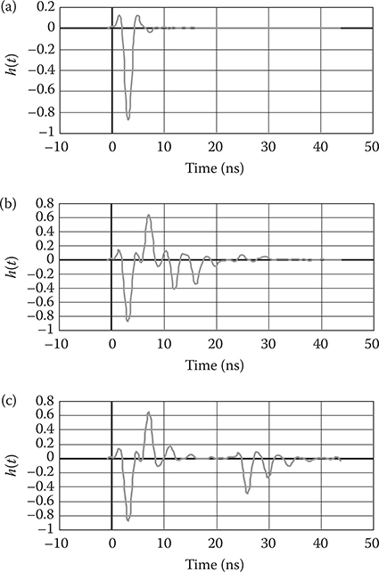
FIGURE 8.6
Calculated reflected time responses from the model 3 with an incident angle of 20° and 1-ns signal duration and different air layers: (a) for absence of an air layer, (b) for thickness of air layer 1 m, and (c) for thickness of air layer 3 m.

In the work [3], the PC physical optics approximation has been obtained under the following limitations: (1) Only the monostatic case was considered and (2) the terminator path or “light-shadow” boundary was a plane curve with the plane orthogonal to the illumination direction. At the same time, there are simple examples of the smooth closed convex surfaces with nonplanar terminators. An ellipsoid illuminated in the arbitrary direction ${\vec{R}}^{0}$ has the same terminator as a plane curve (ellipse), so its plane is orthogonal to ${\vec{R}}^{0}$ only when ${\vec{R}}^{0}$ is parallel to one of the main axes of the ellipsoid.

Separation of terms corresponding to the terminator break of the current density in a physical optics approximation was performed under the same conditions that is, only in the monostatic case and when the terminator path is a plane curve [4]. Research methods in works [3] and [4] are essentially based on the conditions (1) and (2) above, so they cannot be used in the absence of each of them.

Below, we propose the PC calculation method for the physical optics approximation for a smooth convex, perfectly conducting scatterer. This method allows calculating the PC in a bistatic case for an arbitrary orientation of the terminator plane relative to the illumination direction. The method is also valid for the nonplanar terminator case [10]. We can use the typical example of diffraction on a triaxial ellipsoid to describe bistatic scattering. This permits identifying the contribution introduced into PC by terminator breaks using the localization of the PC asymptotics near the terminator path. This contribution corresponds to the current density break on the terminator near moments of the first and the last contacts of the “intermediate” wave. The “intermediate” wave vector is equal to the difference of the unit vectors of illumination and reception direction.

The terminator break in PC has a nonlocalized structure in the monostatic scattering and a terminator plane orthogonal to the illumination direction as described in the work [4]. In this case, the contact of incident plane wave takes place simultaneously for all points of terminator path. The main terms of this “terminator path” asymptotics have been separated. These terms do not have physical sense and introduce infinite breaks to PC. Removal of such break terms regularizes the PC calculated in the physical optics approximation. In addition, this approximation noticeably increases the accuracy of the PC physical optics approximation on the time interval before the arrival of the diffraction wave rounding the shadow region.

8.3.1 Problem Solution Method

We consider the field $\vec{E} (\vec{x}, k)$ , $\vec{H} (\vec{x}, k)$ scattered by a perfectly conducting object bounded by the smooth closed convex surface S and probed by the plane wave

$\begin{array}{l} {\vec{E}}^{0} ({\vec{R}}^{0}, k) = \vec{p} \exp (i k ({\vec{R}}^{0} \cdot \vec{x} + a), \\ {\vec{H}}^{0} ({\vec{R}}^{0}, k) = \sqrt{\frac{ε_{0}}{μ_{0}}} [{\vec{R}}^{0} \times \vec{p}] \exp (i k ({\vec{R}}^{0} \cdot \vec{x} + a)), \end{array} (8.31)$

where $\vec{p} \cdot {\vec{R}}^{0} = 0$ and a is the distance between the origin of coordinates O associated with the object and the illumination source. Time dependence is determined by the factor exp(−iωt). From the strict vector integral formulae of Green’s type [5], the well-known asymptotic representation of the scattered field ${\vec{H}}^{r} ({\vec{r}}^{0}, k)$ in the far zone and in an arbitrary direction ${\vec{r}}^{0}$ is as follows:

${\vec{H}}^{r} ({\vec{r}}^{0}, k) \sim \frac{\exp (i k r)}{4 π r} i k \int_{S} (\vec{K^{}} \times {\vec{r}}^{0}) \exp (- i k ({\vec{r}}^{0} \cdot \vec{x})) d S, (8.32)$

where r is the distance between the origin of coordinates O and reception point, $\vec{K} = \vec{n} \times \vec{H}$ is an equivalent density of the surface current, $\vec{H}$ is a vector of the magnetic intensity of the full field, and $\vec{n}$ is an internal normal unit to S.

In the physical optics approximation, $\vec{K}$ is assumed to be approximately equal to $2 (\vec{n} \times {\vec{H}}^{0})$ on the “illuminated” part S′ of the surface S and to zero on the “nonilluminated” part. So the approximate formula (Equation 8.32) for the magnetic field intensity of the scattered field takes the form

${\vec{H}}^{r} ({\vec{r}}^{0}, k) \sim i k \int_{S'} \exp (i k Φ (\vec{x}, {\vec{r}}^{0})) \vec{A} (\vec{x}, {\vec{r}}^{0}) d S, (8.33)$

where

$Φ (\vec{x}, {\vec{r}}^{0}) = ({\vec{R}}^{0} - {\vec{r}}^{0}) \cdot (\vec{x} + r + a), (8.34)$

$\vec{A} (\vec{x}, {\vec{r}}^{0}) = \sqrt{\frac{ε_{0}}{μ_{0}}} \frac{1}{2 π r} [({\vec{R}}^{0} \times \vec{p}) ({\vec{r}}^{0} \cdot \vec{n}) - ({\vec{R}}^{0} \vec{p} {\vec{r}}^{0}) \vec{n}] . (8.35)$

The PC of the object becomes

${\vec{H}}^{r} ({\vec{r}}^{0}, t) \approx - \frac{\partial}{\partial t} \int_{S'} δ (t - Φ (\vec{x}, {\vec{r}}^{0})) \vec{A} (\vec{x}, {\vec{r}}^{0}) d s, (8.36)$

which is an operational original spectral transform of which the high-frequency approximation is determined by Equation 8.33. Here, δ(t) is a Dirac delta-function. We can rewrite Equation 8.36 in the equivalent form

${\vec{H}}^{r} ({\vec{r}}^{0}, t) \approx - \frac{\partial^{2}}{\partial^{2}} \int_{S_{t}} \vec{A} (\vec{x}, {\vec{r}}^{0}) d s, (8.37)$

where

$S_{t} : {\vec{x} \in S^{'} \cap P_{t}}, P_{t} = {\vec{x} : Φ (\vec{x}, {\vec{r}}^{0}) \leq t} . (8.38)$

Introducing the vector function

$\vec{N} = \int_{S_{t}} \vec{n} d S (8.39)$

and substituting Equation 8.35 in Equation 8.37, we obtain

${\vec{H}}^{r} ({\vec{r}}^{0}, t) = - \sqrt{\frac{ε_{0}}{μ_{0}}} \frac{1}{2 π r} [({\vec{R}}^{0} \times \vec{p}) ({\vec{r}}^{0} \cdot \frac{\partial^{2} \vec{N}}{{\partial t}^{2}}) - ({\vec{R}}^{0} \vec{p} {\vec{r}}^{0}) \frac{\partial^{2} \vec{N}}{\partial^{2}}] . (8.40)$

Note that, as it follows from Equation 8.6, ${\vec{H}}^{r} ({\vec{r}}^{0}, t) = 0$ at t < t_min and at t > t_max, where

$\begin{matrix} \begin{matrix} t_{min} = \min_{\bar{x} \in S'} Φ (\vec{x}, {\vec{r}}^{0}) & and \end{matrix} & t_{max} = \min_{\bar{x} \in S'} \end{matrix} Φ (\vec{x}, {\vec{r}}^{0})$

and hence

${\vec{H}}^{r} ({\vec{r}}^{0}, k) = \int_{t_{\min}}^{t_{\max}} \exp (i k t) {\vec{H}}^{r} ({\vec{r}}^{0}, t) d t .$

Thus, to obtain the response ${\vec{H}}^{r} ({\vec{r}}^{0}, t)$ it is sufficient to calculate the function $\partial^{2} \vec{N} / \partial t^{2}$ on the time interval t ∈ (t_min, t_max). Values t_min and t_max determine the time boundaries of PC, outside of which the PC is identically equal to zero in physical optics approximation. Values t_min, t_max are the moments of arrival of the wavefronts (surfaces of the field break) limiting the pulse response.

If $\partial^{2} \vec{N} / \partial t^{2}$ has continuity breaks inside the interval t ∈ (t_min, t_max), then the wavefronts in ${\vec{H}}^{r} ({\vec{r}}^{0}, t)$ can correspond to these moments. For example, for ellipsoid scattering, the “intermediate” wavefront corresponds to the fist contact of the plane wave $Φ (\vec{x}, {\vec{r}}^{0}) = t$ with the terminator path.

After performing differentiation in Equation 8.39, we obtain

$\frac{\partial \vec{N}}{\partial t} = lim_{Δ t \to 0} \frac{1}{Δ t} [\int_{S_{t + Δ t}} \vec{n} d s - \int_{S_{t}} \vec{n} d s] = \lim_{Δ t \to 0} \frac{1}{Δ t} \int_{s_{t + Δ t} / s_{t}} \vec{n} d s . (8.41)$

Taking into account that

$d S = \frac{d t d l}{\sqrt{1 - ({\vec{l}}^{0} \cdot \vec{n})^{2}}}, {\vec{l}}^{0} = \frac{{\vec{R}}^{0} - {\vec{r}}^{0}}{| {\vec{R}}^{0} - {\vec{r}}^{0} |},$

where dl is the unit of curve Γ(t) (intersection of the plane $Φ (\vec{x}, {\vec{r}}^{0}) = t$ with the surface S′), we can obtain

$\frac{\partial \vec{N}}{\partial t} = \int_{Γ (t)} \frac{\vec{n}}{\sqrt{1 - ({\vec{l}}^{0} \cdot \vec{n})^{2}}} d l . (8.42)$

Thus, for the calculation of $\partial^{2} \vec{N} / \partial t^{2}$ , it is necessary to differentiate the right part of Equation 8.42 by t. The obtained expression can be used for the calculation of the object response to Heaviside step function χ(t). We consider the calculation of functions $\partial \vec{N} / \partial t$ and $\partial^{2} \vec{N} / \partial t^{2}$ for the special case when S is the surface of a triaxial ellipsoid.

8.3.2 Ellipsoid Pulse Characteristics

The ellipsoid with surface S satisfies the equation

$\begin{matrix} | A^{- 1} \vec{x} |^{2} = 1, & A = diag (a_{1}, a_{2}, a_{3}) \end{matrix} . (8.43)$

Therefore, the relation in Equation 8.42 can be rewritten in the form

$\frac{\partial \vec{N}}{\partial t} = \int_{ϕ_{0} (t')}^{π - ϕ_{0} (t')} \vec{f} (ϕ, t') d ϕ, (8.44)$

where

$t' = \frac{t - r - a}{| A ({\vec{R}}^{0} - {\vec{r}}^{0}) |} and φ_{0} (t^{'}) = {\begin{cases} - \frac{π}{2}, - 1 \leq t^{'} < t_{0}^{'} \\ arcsin (\frac{t^{'}}{\sqrt{1 - {t^{'}}^{2}}} . \frac{1}{α}), t_{0}^{'} \leq t^{'} \leq t_{max}^{'} \end{cases} .$

The values $t_{max}^{'} = - 1$ and $t_{max}^{'} = - α / \sqrt{1 + α^{2}}$ correspond to t_min and t_max, and the value $t_{0}^{'} = - α / \sqrt{1 + α^{2}} = - t_{max}^{'}$ corresponds to the moment t₀, starting from which the surface $Φ (\vec{x}, {\vec{r}}^{0}) = t$ intersects the terminator plane. Here

$α = \frac{\vec{Q} \cdot {\vec{v}}^{0}}{\vec{Q} \cdot {\vec{L}}^{0}}' \vec{Q} = A^{- 1} {\vec{R}}^{0}, {\vec{v}}^{0} = {\vec{u}}^{0} \times {\vec{L}}^{0}, {\vec{u}}^{0} = - \frac{{\vec{L}}^{0} \times \vec{Q}}{| {\vec{L}}^{0} \times \vec{Q} |}' {\vec{L}}^{0} = - \frac{A {\vec{l}}^{0}}{| A {\vec{l}}^{0} |} .$

It is easy to show that α ≥ 0. In reality, we note that

$\begin{matrix} \vec{Q} \cdot {\vec{L}}^{0} = - \frac{{\vec{R}}^{0} ({\vec{R}}^{0} - {\vec{r}}^{0})}{| A ({\vec{R}}^{0} - {\vec{r}}^{0}) |} = - \frac{1 - ({\vec{R}}^{0} \cdot {\vec{r}}^{0})}{| A ({\vec{R}}^{0} - {\vec{r}}^{0}) |} < 0, \\ \vec{Q} \cdot {\vec{v}}^{0} = - \frac{| \vec{Q} |^{2} - (\vec{Q} \cdot {\vec{L}}^{0})^{2}}{| {\vec{L}}^{0} \times \vec{Q} |} \leq 0 \end{matrix}$

and hence α ≥ 0.

The functions in the right part of Equation 8.44 have the form

$\begin{matrix} \vec{f} (ϕ, t') = & R (ϕ) A^{- 1} [t' {\vec{L}}^{0} + \sqrt{1 - t^{' 2}} \vec{Φ} (ϕ)], \\ Φ (ϕ) = & {\vec{u}}^{0} \cos ϕ + {\vec{ν}}^{0} \sin ϕ, \\ R (ϕ) = & \begin{matrix} [\frac{| A \vec{Φ}' (ϕ) |^{2}}{| A^{- 1} \vec{Φ} |^{2} - ({\vec{l}}^{0} A^{- 1} \vec{Φ})^{2}} ⌉^{\frac{1}{2}} . \end{matrix} \end{matrix} (8.45)$

After some easy transformations, the relation in Equation 8.44 can be represented in the form

$\frac{\partial \vec{N}}{\partial t} = [χ (t' + 1) \int_{0}^{2 π} \vec{f} (φ, t') d φ - χ (t' - t_{0}') \int_{π - φ_{0} (t^{'})}^{2 π + φ_{0} (t^{'})} \vec{f} (φ, t^{'}) d φ] χ (t_{max}^{'} - t^{'}) . (8.46)$

By differentiating Equation 8.46 with respect to t, we obtain the following equation after simplifications:

$\begin{array}{l} \frac{\partial^{2} \vec{N}}{\partial t^{2}} = \frac{χ (t_{max}^{'} - t')}{| A ({\vec{R}}^{0} - {\vec{r}}^{0}) |} {δ (t' + 1) \int_{0}^{2 π} \vec{f} (ϕ, - 1) d ϕ + χ (t' + 1) \int_{0}^{2 π} \frac{\partial \vec{f} (ϕ, t')}{\partial t'} d ϕ - \\ - χ (t' - t_{0}') [\int_{π - ϕ_{0} (t')}^{2 π + ϕ_{0} (t')} \frac{\partial \vec{f} (ϕ, t')}{\partial t'} d ϕ + ϕ_{0}^{'} (t') (\vec{f} (2 π + ϕ_{0} (t'), t') + \vec{f} (π - ϕ_{0} (t'), t'))]} \end{array} (8.47)$

Here

$φ_{0}' (t) = [(1 - t^{' 2}) \sqrt{1 + α^{2}} \sqrt{t_{\max}^{' 2} - t^{' 2}}]^{- 1}, (8.48)$

for $t_{0}^{'} < t^{'} < t_{max}^{'}$ .

Note that the expression in the right part of Equation 8.47 has infinite breaks for $t^{'} = t_{0}^{'}$ and $t^{'} = t_{max}^{'}$ stipulated by the behavior of the function $φ_{0}^{'} (t^{'})$ . These breaks were caused by the nonadequate description of the surface current density near the terminator path in physical optics approximation.

We remove these nonexisting breaks, deducing the main terms of the functional asymptotics in the neighborhood of points $t^{'} = t_{0}^{'}$ and $t^{'} = t_{max}^{'}$ from the right-hand part of Equation 8.47, that is, deducing the vector function:

$\vec{I} (t') = - \frac{[1 + α^{2}]^{\frac{3}{4}}}{| A ({\vec{R}}^{0} - {\vec{r}}^{0}) |} \sqrt{\frac{2}{α}} [\frac{\vec{f} (\frac{3 π}{2}' t_{0}')}{\sqrt{t' - t_{0}'}} + \frac{\vec{f} (\frac{π}{2}, t_{\max}^{'})}{\sqrt{t_{\max}^{'} - t'}}] χ (t_{max}^{' 2} - t^{'} 2) . (8.49)$

The vector function $\partial^{2} \vec{N} / \partial t^{2}$ derived in such a way is continuous, but it has derivatives, becoming infinity at points $t^{'} = t_{0}^{'}$ and $t^{'} = t_{max}^{'}$ .

8.3.3 Transient Response Calculation of the Aircraft Model in a Bistatic Case

If the target PC ${\vec{H}}^{r} ({\vec{r}}^{0}, t)$ is known, we can find the response of the complex target to the probing signal Ω(t) by convolution:

$H^{s} ({\vec{r}}^{0}, t) = \int_{- \infty}^{\infty} Ω (s) {\vec{H}}^{r} ({\vec{r}}^{0}, t - s) d s . (8.50)$

Let us suppose that Ω(s) ≡ 0 for s < 0 and s > τ_p and ${\vec{H}}^{r} ({\vec{r}}^{0}, t) = 0$ for t < t_min. In this case, Equation 8.50 can be rewritten as

${\vec{H}}^{s} ({\vec{r}}^{0}, t) = \int_{0}^{\min {t - t_{\min}, τ_{p}}} Ω (s) {\vec{H}}^{r} ({\vec{r}}^{0}, t - s) d s . (8.51)$

Taking into account Equation 8.40 obtaining the transient response required calculating the vector function

$\vec{K} (t) = \int_{0}^{\min {t - t_{\min}, τ_{p}}} Ω (s) \frac{\partial^{2} \vec{N}}{{\partial t}^{2}} (t - s) d s . (8.52)$

Moreover, the value t − t_min in the upper limit of integration should be understood as t − t_min + 0, so the “peak” of δ-function in $\partial^{2} \vec{N} / \partial t^{2}$ is placed within the integration interval.

The calculation in Equation 8.52 is easy to perform when integration is carried out in parts. In this case,

$\vec{K} (t) = \int_{0}^{\min {t - t_{\min}, τ_{p}}} Ω' (s) \frac{\partial \vec{N}}{\partial t} (t - s) d s . (8.53)$

The expression in the right part of Equation 8.53 is preferable since the calculation of $\partial \vec{N} / \partial t$ is essentially simpler than the calculation of $\partial^{2} \vec{N} / \partial t^{2}$ .

Consider an aircraft model shown in Figure 8.7 containing m triaxial ellipsoids I₁, I₂, . . . , I_m (m = 5). In this case, obtaining of $\partial \vec{N} / \partial t$ is reduced to the following steps:

Determine $t_{min}^{l}$ , $t_{max}^{l}$ (l = 1, 2, …, m) for each ellipsoid.
If the current value of time t lies inside the corresponding interval ( $t_{min}^{l}$ , $t_{max}^{l}$ ), then we can calculate for lth ellipsoid, the radius vector of point ${\vec{X}}_{l_{j}}$ on curve Γ_t corresponding to polar angle φ₀ (t′) < φ_j < π − φ₀ (j = 1, 2,...,J_l).
For each point with radius vector ${\vec{X}}_{l_{j}}$ (j = 1, 2,..., J_l of lth ellipsoid) the visibility test has been carried out [4], that is, it checks whether the point is shadowed by other ellipsoids or not.
The calculation of integral in $\partial \vec{N} / \partial t$ is performed. In this case, the curve Γ_t includes the parts of curves Γ_t of separate ellipsoids composing the aircraft model.
The calculation of Equation 8.53 can be performed by numerical integration. Taking into account the smooth nature of function Ω′(s), the numerical integration can be carried out by trapezium formula.

In accordance with the proposed method, the calculations of transient responses of the aircraft model shown in Figure 8.7 have been obtained.

Images

FIGURE 8.7
Ellipsoidal aircraft model for PC computation.

We use the following sizes of ellipsoid half-axes:

I₁ : a₁ = 1.25 m, a₂ = 1.25 m, a₃ = 9 m,

I₂ : a₁ = 0.5m, a₂ = 11m, a₃ = 2m,

I₃ : a₁ = 0.5m, a₂ = 11m, a₃ = 2m,

I₄ : a₁ = 0.3 m, a₂ = 3 m, a₃ = 1m,

I₅ : a₁ = 3 m, a₂ = 0.3m, a₃ = 1m.

The centers of ellipsoids I₁, I₂, I₃ were placed at the origin of coordinate system OX₁X₂X₃ and the centers of ellipsoids I₄ and I₅ were located at 7.6 m from origin O along the axis OX₃.

We used the short videopulse shown in Figure 8.8 with the duration of τ_p as time-dependence probing signal:

$Ω (t) = \frac{1}{\sqrt{π} τ_{p}} \exp (- \frac{t^{2}}{τ_{p}^{2}}) - \frac{1}{1.5 \sqrt{π} τ_{p}} \exp (- \frac{t^{2}}{(1.5 τ_{P})^{2}}) . (8.54)$

Figures 8.9 and 8.10 show the model responses [time dependences of normalized electric field e(t)] for the pulses of duration τ_p = 3 and 10 ns, respectively. The electrical vector of the probing signal lies in the OX₂X₃ plane.

In Figures 8.9 and 8.10, “a” and “b” plots correspond to responses for “front” probing along the model axis as shown in Figure 8.7. The “c” and “d” plots correspond to probing at an angle 30° to the model axis. The “a” and “c” plots have been obtained for bistatic angle 20°. The “b” and “d” charts have been obtained for bistatic angle 40°.

The videopulses have physical lengths of 0.9 m for the 3-ns case and of 3 m for the 10-ns case. Note that the target response contains less information when the videopulse’s physical length approximates the physical size of the target. We can see that for the shortest probing signal allowed to determine responses from separated parts of the model. A longer probing signal has less resolution and produces less response from the aircraft model.

Images

FIGURE 8.8
The time dependence of videopulse probing signal.

Images

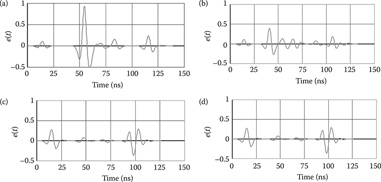
FIGURE 8.9
Responses of an aircraft model (r_p = 3 ns), which are shown for front- and 30° side probes with bistatic angles of 20° and 40°. This shows how the reflected signal varies with the receiver conditions for a complex geometric target: (a) for “front” probing and bistatic angle 20°, (b) for “front” probing and bistatic angle 40°, (c) for probing at an angle 30° to the model axis and bistatic angle 20°, and (d) for probing at an angle 30° to the model axis and bistatic angle 40°.

8.4 Pulse Signal Scattering from Perfectly Conducting Object Located near the Uniform Half-Space

This section presents an approximation method for calculating the pulse signal backscattering from perfectly conducting electrically large objects (with small curvatures) placed near the boundary of uniform half-space (with complex electrical parameters). The calculation results may be used for obtaining a priori information about scattering characteristics of ground objects in radar detection and recognition.

The method uses field integral representations obtained from Lorenz’s lemma. These representations take into account the electromagnetic interactions between a perfectly conducting scatterer (method for calculation presented in second part) and uniform half-space boundary (first part). Then a high-frequency approximation of object transient characteristic (for backscattering in a far-field zone) is obtained by taking account of the half-space boundary presence. Note that the behavior of a transient pulse response near its wavefront corresponds to short-wave asymptotics in the frequency domain. It is well known that such asymptotics correspond to the short-wave asymptotics in the frequency domain. Transient characteristic allows obtaining the object response on the arbitrarily shaped plane pulse wave.

Images

FIGURE 8.10
Responses of an aircraft model (r_p = 10ns): (a) for “front” probing and bistatic angle 20°, (b) for “front” probing and bistatic angle 40°, (c) for probing at an angle 30° to the model axis and bistatic angle 20°, and (d) for probing at an angle 30° to the model axis and bistatic angle 40°. Note how the physically longer pulse with less bandwidth produces a simpler response from the target than the shorter (3 ns) pulse shown in Figure 8.9. Decreased range resolution produces a target response different from that shown in Figure 8.9.

In the general case, the calculation of the pulse response of a perfectly conducting object located near ground surface means determining the fields scattered by the object in free space for different directions of pulse incidence.

The method for calculation of PC of smooth, perfectly conducting objects in bistatic case, based on a physical optics approximation [6], has been proposed in the work [7].

8.4.1 Formulation of the Problem and the Main Calculation Relations

Let us consider a perfectly conducting object placed near the ground surface. It is necessary to take into account the mutual interaction in the system “object-half-space with ground parameters.” For this purpose, we need to obtain the integral representations of the fields scattered by such system.

We consider a plane pulse wave (signal)

$\begin{array}{l} {\vec{E}}^{0} ({\vec{R}}^{0}, t) = {\vec{p}}^{0} Q (t + {\vec{R}}^{0} \cdot \vec{x}), \\ {\vec{H}}^{0} ({\vec{R}}^{0}, t) = \sqrt{\frac{β_{0}}{μ_{0}}} [{\vec{p}}^{0} \times {\vec{R}}^{0}] Q (t + {\vec{R}}^{0} \cdot \vec{x}), \end{array} (8.55)$

which falls on a perfectly conducting object with surface S located above the boundary L of the dielectric half-space V⁺ shown in Figure 8.11. Here, Q(t) is a function of signal time dependence, ${\vec{R}}^{0} = (- sin θ, 0, - cos θ)$ , ${\vec{p}}^{0} = (p_{1}, p_{2}, p_{3})$ and ε⁰, μ⁰ are the permittivity and permeability of the free half-space V^-.

For most of the cases, the multiple rereflections between the object and underlying surface have second-order effects compared to the single reflection from plane L. This part considers the nonresonant case.

Surface S is illuminated by the plane wave of Equation 8.11 and by the wave reflected one time from plane L shown in Figure 8.11, which is needed to obtain the integral representations for fields scattered by such systems.

Let $\vec{ℰ} (x | x_{0}, \vec{p})$ , $\vec{H} (x | x_{0}, \vec{p})$ be a field generated by point dipole located at point x₀ with vector moment p at the presence of half-space V+. The field $\vec{ℰ} (x | x_{0}, \vec{p})$ , $\vec{H} (x | x_{0}, \vec{p})$ follows Maxwell’s equations:

${\begin{cases} \vec{\begin{matrix} \nabla \end{matrix}} \times \vec{ℰ} = j ω μ_{0} \vec{H} \\ \vec{\begin{matrix} \nabla \end{matrix}} \times \vec{H} = - j ω ϵ \vec{ℰ} - j ω \vec{p} δ {(x - x_{0})}^{'} \end{cases} (8.56)$

where

$ε = {\begin{matrix} ε_{0}, x_{0} \in V^{-}, \\ ε_{1,} x_{0} \in V^{+} . \end{matrix}$

If the main part of probing signal spectrum is above 50 MHz, it is possible to neglect the dispersive properties of the absorbing medium with ground parameters [1].

Add the boundary conditions on the plane L

${\vec{ℰ}}_{T}^{+} = {\vec{ℰ}}_{T}^{-}, {\vec{H}}_{T}^{+} = {\vec{H}}_{T}^{-} (8.57)$

to the system of relations in Equation 8.56. Here ${\vec{A}}_{T} = \vec{A} - \vec{n} (\vec{A} \vec{n}), {\vec{B}}_{⊥} = (\vec{n} \times \vec{B})$ , where n is a unit normal to the corresponding boundary.

Images

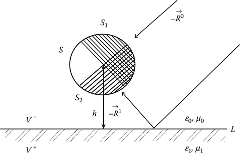
FIGURE 8.11
Geometry of scattering by a perfectly conducting object with surface S located above the boundary of half-space L.

The considered field $\vec{E} (\vec{x}), \vec{H} (\vec{x})$ is generated by the distribution of current volume density $\vec{J}$ in the region V^- in the presence of the half-space V+ and the perfectly conducting scatterer S. For this case, Maxwell’s equations are

${\begin{cases} \vec{\nabla} \times \vec{E} = j ω μ_{0} \vec{H}, \\ \vec{\nabla} \times \vec{H} = - j ω ϵ \vec{E} + \vec{J} . \end{cases} (8.58)$

Note that ∂V^- = L ∪ S is the boundary of the region V^- shown in Figure 8.11. Boundary conditions at plane L

${\vec{E}}_{T}^{+} = {\vec{E}}_{T}^{-}, {\vec{H}}_{T}^{+} = {\vec{H}}_{T}^{-} (8.59)$

need to be added by boundary conditions at the surface S

${\vec{E}}_{T} | s = 0. (8.60)$

Let us use Lorenz’s lemma for fields $(\vec{E} (\vec{x}), \vec{H} (\vec{x}))$ and $(\vec{ℰ} (x | x_{0}, \vec{p}), \vec{H} (x | x_{0}, \vec{p}))$ in the region V⁻ for x₀ ∈ V−, so that

$\int_{L} ({\vec{E}}_{T}^{-} . {\vec{H}}_{⊥}^{-} - {\vec{ℰ}}_{T}^{-} . {\vec{H}}_{⊥}^{-}) d l - \int_{S} {\vec{E}}_{T}^{-} \cdot {\vec{H}}_{⊥}^{-} d s = - \int_{V^{-}} (j ω \vec{p} δ (x - x_{0}) {\vec{E}}_{T}^{-} + \vec{J} \cdot \vec{ℰ}) d v . (8.61)$

By using filtering properties of δ–function and superposition principle, we obtain the representation

$j ω \vec{p} (\vec{E} (x_{0}) - \vec{ℰ} (x_{0})) = \int_{S} {\vec{ℰ}}_{T} (x | x_{0}, \vec{p}) \cdot {\vec{H}}_{⊥} (x) d s - \int_{L} ({\vec{E}}_{T}^{-} . {\vec{H}}_{⊥}^{-} - {\vec{ℰ}}_{T}^{-} \cdot {\vec{H}}_{⊥}^{-}) d l, (8.62)$

where $\vec{ℰ} (x_{0})$ is a field generated by the given distribution of currents $\vec{J}$ in half-space V- without scatterer S.

By applying Lorenz’s lemma to the same fields in the region V⁺, we obtain

$0 = \int_{L} ({\vec{E}}_{T}^{+} \cdot {\vec{H}}_{⊥}^{+} - {\vec{E_{T}}}^{+} \cdot {\vec{H}}_{⊥}^{+}) d l . (8.63)$

By adding the relations of Equations 8.62 and 8.63 term by term and taking into account the boundary conditions of Equations 8.59, 8.60, and 8.61, we obtain the following integral representation for field $\vec{E} (x_{0})$

$j ω \vec{p} (\vec{E} (x_{0}) - \vec{E} (x_{0})) = \int_{S} \vec{ℰ} (x | x_{0}, \vec{p}) \cdot {\vec{H}}_{⊥} (x) d s . (8.64)$

Let ${\vec{x}}_{0}$ be a vector with length x₀ directed to the radiation source

${\vec{x}}_{0} = x_{0} {\vec{R}}^{0}, (8.65)$

where ${\vec{R}}^{0}$ is a unit vector.

If x₀ → ∞, then the representation of Equation 8.64 has the following form:

$j ω \vec{p} (\vec{E} ({\vec{R}}^{0}) - \vec{E} ({\vec{R}}^{0})) = \int_{S} {\vec{E}}_{T} (x | {\vec{R}}^{0}, \vec{p}) \cdot {\vec{H}}_{⊥} (x) d s . (8.66)$

Here, $\vec{E} (x | {\vec{R}}^{0}, \vec{p})$ is the field generated by the plane wave

${\vec{ℰ}}_{0} (x | {\vec{R}}^{0}, \vec{p}) = k_{0}^{2} ω \sqrt{\frac{μ_{0}}{ε_{0}}} {\vec{p}}^{0} \exp (- j k_{0} ({\vec{R}}^{0} \cdot \vec{x})) \cdot Ω (k_{0} x_{0}), (8.67)$

where

$Ω (k_{0}, x_{0}) = \frac{1}{4 π} \frac{\exp (j k_{0} x_{0})}{k_{0} x_{0}} .$

The wave $\vec{ℰ} (x | {\vec{R}}^{0}, \vec{p})$ propagates in the direction − ${\vec{R}}^{0}$ in the presence of the half-space V+ only (without scatterer S). In this case, $\vec{E} ({\vec{R}}^{0})$ , $\vec{ℰ} ({\vec{R}}^{0})$ are the back-scattered fields in the presence and absence of the scatterer S, respectively.

The plane wave of Equation 8.67 originates by the limit process in the vector function:

$\begin{matrix} \vec{ℰ} (x | x_{0}, \vec{p}) = \frac{1}{ϵ_{0}} [\vec{\nabla} (\vec{p} {\vec{\nabla}}_{g}) + k_{0}^{2} \vec{p} g], & (g (x, x_{0}) = \frac{exp ({j k}_{0} | \vec{x} - {\vec{x}}_{0} |)}{4 π | \vec{x} - {\vec{x}}_{0} |}) . \end{matrix}$

The wave of Equation 8.67 corresponds to the field of the dipole located in free space at point ${\vec{x}}_{0} \in V^{-}$ if $| {\vec{x}}_{0} | \to \infty$ . The following asymptotic expansion of function g(x, x₀) for x₀ → ∞ has been used:

$g (x, x_{0}) ~ k_{0} Ω (k_{0} x_{0}) exp (- j k_{0} ({\vec{R}}^{0} \cdot \vec{x})) .$

In the general case, the plane wave of Equation 8.67 falls on the plane L arbitrarily. Then the field scattered in direction ${\vec{R}}^{0}$ is equal to zero $(\vec{ℰ} ({\vec{R}}^{0}) = 0)$ Thus, expression for the field above the surface L without the scatterer S has the following form:

$\vec{ℰ} (x | {\vec{R}}^{0}, \vec{p}) = k_{0}^{2} ω \sqrt{\frac{μ_{0}}{ϵ_{0}}} [{\vec{p}}^{0} exp (- j k_{0} ({\vec{R}}^{0} \cdot \vec{x})) + {\vec{p}}^{1} exp (- j k_{0} ({\vec{R}}^{1} \cdot \vec{x}))] Ω (k_{0} x_{0}), (8.68)$

where $- {\vec{R}}^{1} = - {\vec{R}}^{0} + 2 \vec{n} ({\vec{R}}^{0} \cdot \vec{n})$ is a propagation direction of the wave reflected from surface L and ${\vec{p}}^{1}$ is an unknown vector to be calculated, for example, by the method set out in the work [7].

Images

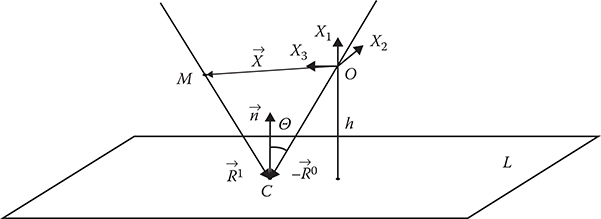
FIGURE 8.12
Calculation of the phase delays of the wave rereflected from the plane L.

It is necessary to take into account the phase delays associated with reflection from the boundary L. Set a point M at the object surface with radius vector $\vec{x}$ in some frame of reference OX₁X₂X₃. Let C be a point of a mirror reflection on the plane L. The reflected beam from point C passes through the point M on S shown in Figure 8.12.

The plane L is described by the equation:

$(\vec{x} \cdot \vec{n}) + h = 0, (8.69)$

where h is the distance from the plane L to the origin of the coordinate system O.

Let $\vec{c} = \vec{OC} = \vec{x} - λ {\vec{R}}^{1}$ , $\vec{ξ} = \vec{CM} = \vec{x} - \vec{c} = λ {\vec{R}}^{1}$ where λ is determined from the condition that the point C is placed on the plane L:

$λ = \frac{(\vec{x} \cdot \vec{n}) + h}{({\vec{R}}^{1} \cdot \vec{n})} . (8.70)$

So, the incident wave of Equation 8.67 is represented in the form

$\begin{matrix} {\vec{ℰ}}_{0} (x | {\vec{R}}^{0}, \vec{p}) = & Ω (k_{0} x_{0}) k_{0}^{2} ω \sqrt{\frac{μ_{0}}{ϵ_{0}}} {\vec{p}}_{0} exp (- {j k}_{0} ({\vec{R}}^{0} \cdot (\vec{c} + \vec{ξ}))) \\ = & Ω (k_{0} x_{0}) k_{0}^{2} ω \sqrt{\frac{μ_{0}}{ϵ_{0}}} {\vec{p}}^{0} exp (- j k_{0} ({\vec{R}}^{0} \cdot \vec{c})) exp (- j k_{0} ({\vec{R}}^{0} \cdot \vec{c})) exp (- j k_{0} (\vec{R} \cdot \vec{ξ})) = {\hat{\vec{p}}}^{0} exp (- j k_{0} ({\vec{R}}^{0} \cdot \vec{ξ})) \end{matrix}$

and the reflected wave, respectively, in the form

$\begin{matrix} \vec{ℰ} (x | {\vec{R}}^{1}, {\vec{p}}^{1}) = & {\hat{\vec{p}}}^{1} exp (- j k_{0} ({\vec{R}}^{1} \cdot \vec{ξ})) = Ω {(k_{0} x_{0}) k}_{0}^{2} ω \sqrt{\frac{μ_{0}}{ϵ_{0}}} {\vec{p}}^{1} exp (- {j k}_{0} ({\vec{R}}^{0} \cdot \vec{c})) exp (- j k_{0} ({\vec{R}}^{1} \cdot \vec{ξ})) \\ = & Ω (k_{0} x_{0}) k_{0}^{2} ω \sqrt{\frac{μ_{0}}{ϵ_{0}}} {\vec{p}}^{0} exp (- j k_{0} (({\vec{R}}^{0} \cdot {\vec{R}}^{1}) \cdot \vec{c} + {\vec{R}}^{1} \cdot \vec{x})) . \end{matrix}$

Thus, the total field at the point $\vec{x}$ at the surface of the object S with taking into account the phase delays can be written:

$\vec{ℰ} (x | \overset{\to 0}{R}, \vec{p}) = k_{0}^{2} ω \sqrt{\frac{μ_{0}}{ε_{0}}} [\overset{\to 0}{p} \exp (- j k_{0} (\overset{\to 0}{R} \cdot \vec{x})) + \overset{\to 1}{p} \exp (- j k_{0} (({\vec{R}}^{0} - {\vec{R}}^{1}) \cdot \vec{c} + {\vec{R}}^{1} \cdot \vec{x}))] Ω (k_{0} x_{0}) . (8.71)$

By using Equation 8.71, we obtain from Equation 8.66

$\begin{matrix} \vec{p} \cdot \vec{E} ({\vec{R}}^{0}) = & - j Ω (k_{0} x_{0}) k_{0}^{2} \sqrt{\frac{μ_{0}}{ε_{0}}} \times \int_{S} [{\vec{p}}^{0} \exp (- j k_{0} ({\vec{R}}^{0} \cdot \vec{x})) \\ + \overset{\to 1}{p} \exp (- j k_{0} (({\vec{R}}^{0} - {\vec{R}}^{1}) \cdot \vec{c} + {\vec{R}}^{1} \cdot \vec{x}))] {\vec{H}}_{⊥} (\vec{x}) d s . \end{matrix} (8.72)$

Note that ${\vec{H}}_{⊥} (\vec{x})$ is the surface current density on S generated by the plane wave propagated in the direction $- {\vec{R}}^{0}$ in the presence of boundary L of half-space V+. The presence of half-space V+ in the considered system gives the additional wave (reflected from the plane L and propagated in the direction $- {\vec{R}}^{1}$ ) that is incident on surface S. So two mutually intersecting (in the general case) illuminated regions S₁ and S_s are localized on the surface of the object as shown in Figure 8.11. In the physical optics approximation, the surface current density in the region S can be expressed in the form

${\vec{H}}_{⊥} (\vec{x}) = {\begin{matrix} 2 \vec{n} \times {\vec{H}}_{1}^{0}, & \vec{x} \in S_{1}, \\ 2 \vec{n} \times {\vec{H}}_{2}^{0}, & \vec{x} \in S_{2}, \end{matrix} (8.73)$

where

$\begin{array}{l} {\vec{H}}_{1}^{0} = ({\vec{p}}^{0} \times {\vec{R}}^{0}) \sqrt{\frac{{\underline{ε}}_{0}}{μ_{0}}} \exp (- j k_{0} ({\vec{R}}^{0} \cdot \vec{x})), \\ {\vec{H}}_{2}^{0} = ({\vec{p}}^{1} \times {\vec{R}}^{1}) \sqrt{\frac{ε_{0}}{μ_{0}}} \exp (- j k_{0} ({\vec{R}}^{0} - {\vec{R}}^{1}) \cdot \vec{c}) \exp (- j k_{0} ({\vec{R}}^{1} \cdot \vec{x})) . \end{array} (8.74)$

The expression in Equation 8.72 can be transformed into a sum of two surface integrals:

$\begin{array}{l} \vec{p} \cdot \vec{E} ({\vec{R}}^{0}) = - {jk}_{0} \times {\int_{S_{1}} [A_{0} (\vec{x}) exp (- {jk}_{0} (2 {\vec{R}}^{0} \cdot \vec{x} - r)) + A_{1} (\vec{x}) exp (- {jk}_{0} (({\vec{R}}^{0} + {\vec{R}}^{1}) \cdot \vec{c} - r))] ds \\ + \int_{S_{2}} [B_{0} (\vec{x}) exp (- {jk}_{0} (2 {\vec{R}}^{1} \cdot \vec{x} + ({\vec{R}}^{0} + {\vec{R}}^{1}) \cdot \vec{c}) - r) + B_{1} (\vec{x}) exp (- {jk}_{0} (({\vec{R}}^{0} + {\vec{R}}^{1}) \cdot \vec{x} + ({\vec{R}}^{0} + {\vec{R}}^{1}) \cdot \vec{c} - r))] ds} . \end{array} (8.75)$

Here, $r = | {\vec{x}}_{0} |$ is a distance from the radiation source to the object, so that

$\begin{array}{l} {\overset{'}{A}}_{0} (\vec{x}) = \frac{1}{2 π r} ({\vec{R}}^{0} \cdot \vec{n}) {\overset{'}{A}}_{1} (\vec{x}) = \frac{1}{2 π r} (({\vec{p}}^{0} \cdot {\vec{p}}^{1}) \cdot ({\vec{R}}^{0} \cdot \vec{n}) - ({\vec{p}}^{1} \cdot {\vec{R}}^{0}) \cdot ({\vec{p}}^{0} \cdot \vec{n})), \\ B_{0} (\vec{x}) = \frac{1}{2 π r} ({\vec{R}}^{1} \cdot \vec{n}) | {\vec{p}}^{1} |^{2}, B_{1} (\vec{x}) = \frac{1}{2 π r} ((p^{0} \cdot {\vec{p}}^{1}) ({\vec{R}}^{1} \cdot \vec{n}) - ({\vec{p}}^{0} \cdot {\vec{R}}^{1}) ({\vec{p}}^{1} \cdot \vec{n})) . \end{array}$

By using the relations between the short-wave asymptotics of the scattered wave (frequency response to plane monochromatic wave of Equation 8.75) and asymptotics of transient response $\vec{ℰ} (t)$ near the wavefront, we obtain

$\vec{p} \cdot \vec{ℰ} (t) = \frac{\partial}{\partial t} {\begin{matrix} \int_{S_{1}} ⌊ A_{0} (\vec{x}) δ (t + 2 ({\vec{R}}^{0} \cdot \vec{x}) - r) + A_{1} (\vec{x}) δ (t + ({\vec{R}}^{0} + {\vec{R}}^{1}) \cdot \vec{x} + ({\vec{R}}^{0} - {\vec{R}}^{1}) \cdot \vec{c} - r) ⌋ d s + \\ \int_{S_{2}} ⌊ B_{0} (\vec{x}) δ (t + 2 ({\vec{R}}^{0} \cdot {\vec{R}}^{1}) \cdot \vec{c} + {\vec{R}}^{1} \cdot \vec{x}) - r) + B_{1} (\vec{x}) δ (t + ({\vec{R}}^{0} + {\vec{R}}^{1}) \vec{x} + ({\vec{R}}^{0} - {\vec{R}}^{1}) \cdot \vec{c} - r) ⌋ d s \end{matrix}} . (8.76)$

Since $({\vec{R}}^{0} - {\vec{R}}^{1}) \cdot \vec{c} = 2 \vec{n} \cos θ \vec{x} - 2 (\vec{x} \cdot \vec{n}) \cos θ - 2 h \cos θ = - 2 h \cos θ$ , Equation 8.76 takes the form

$\vec{p} \cdot \vec{E} (t) = \frac{\partial}{\partial t} {\begin{matrix} \int_{S_{1}} ⌊ A_{0} (\vec{x}) δ (t + 2 ({\vec{R}}^{0} \vec{x}) - r) + A_{1} (\vec{x}) δ (t + ({\vec{R}}^{0} + {\vec{R}}^{1}) \vec{x} - (2 h cos θ) - r) ⌋ d s + \\ \int_{S_{2}} ⌊ B_{0} (\vec{x}) δ (t + 2 ({\vec{R}}^{1} \vec{x}) - (42 h cos θ) - r) + B_{1} (\vec{x}) δ (t + ({\vec{R}}^{0} + {\vec{R}}^{1}) \vec{x} + (2 h cos θ) - r) ⌋ d s \end{matrix}} (8.77)$

Note that the integrals in Equation 8.77 are similar to those in [7]. We use a relation between PC $\vec{ℰ} (t)$ and the transient characteristic $\tilde{\vec{ℰ}} (t)$ , which is the response to the step function,

$\tilde{\vec{ℰ}} (t) = \int \vec{ℰ} (t) d t . (8.78)$

By analogy with [7], we obtain a final expression for a projection of the transient characteristic at an arbitrary direction $\vec{p}$ so that

$\begin{matrix} \vec{p} \cdot \tilde{\vec{ℰ}} (t) = & \int_{Γ_{11} (t)} \frac{A_{0} (\vec{x})}{\sqrt{1 - ({\vec{R}}^{0} \cdot \vec{n})^{2}}} d l + \int_{Γ_{12} (t)} \frac{A_{1} (\vec{x})}{\sqrt{1 - (\frac{({\vec{R}}^{0} + {\vec{R}}^{1}) \cdot \vec{n}}{| {\vec{R}}^{0} + {\vec{R}}^{1} |})^{2}}} d l \\ + \int_{Γ_{21} (t)} \frac{B_{0} (\vec{x})}{\sqrt{1 - ({\vec{R}}^{1} \cdot \vec{n})^{2}}} d l + \int_{Γ_{22} (t)} \frac{B_{1} (\vec{x})}{\sqrt{1 - (\frac{({\vec{R}}^{0} + {\vec{R}}^{1}) \cdot \vec{n}}{| {\vec{R}}^{0} + {\vec{R}}^{1} |})^{2}}} d l, \end{matrix} (8.79)$

where the integral loops Γ_ij (t) are intersections of “illuminated” regions S₁, S₂ with planes determined by different combinations of vectors ${\vec{R}}^{0}$ and ${\vec{R}}^{1}$ so that

$\begin{matrix} Γ_{11} (t) : {S_{1} \cap Π_{1}}, & Γ_{21} (t) : {S_{2} \cap Π_{3}}, \\ Γ_{12} (t) : {S_{1} \cap Π_{2}}, & Γ_{22} (t) : {S_{2} \cap Π_{4}}, \end{matrix}$

where Π_i (i = 1,...,4) are planes given by the equations

$\begin{array}{l} \begin{matrix} \begin{matrix} - 2 {\vec{R}}^{0} \cdot \vec{x} + r = t (Π_{1}), \\ - ({\vec{R}}^{0} + {\vec{R}}^{1}) \cdot \vec{x} + 2 h \cos θ + r = t (Π_{2}), \end{matrix} \\ - 2 {\vec{R}}^{1} \cdot \vec{x} + 4 h \cos θ + r = t (Π_{3}), \end{matrix} \\ - ({\vec{R}}^{0} + {\vec{R}}^{1}) \cdot \vec{x} + 2 h \cos θ + r = t (Π_{4}) . \end{array}$

Here, θ is the incident angle of a plane wave (with respect to boundary L). Thus, the calculation of transient characteristic is reduced to the calculation of four loop integrals.

Obtaining Equation 8.79 from Equations 8.77 and 8.78 is based on the formal limit process in the finite-difference ratio for the calculation of derivatives by t.

Comparison of the obtained expression for the transient characteristic with the integral bistatic transient characteristic of a single object [7] implies that each integral in Equation 8.79 for transient characteristic can be interpreted in terms of a bistatic scattering problem solution. The contribution of the first integral to a transient characteristic is caused by direct reflection of the original plane wave from the surface S (without taking into account the rereflections from the plane L). The remaining integrals contribute to the transient characteristic from other possible combinations of illuminated regions with directions of the wave interacting with the surface S and the plane L.

We can obtain the expression of transient response for arbitrary pulse signal using the transient characteristic $\hat{\vec{ℰ}} (t)$ of a system and the expression for a sounding signal Q(t) with a duration τ:

$\vec{E} (t) = \int_{0}^{T} Q' (s) \tilde{\vec{E}} (t - s) d s, (8.80)$

where T = min {τ, t}

8.4.2 Numerical Results

Some numerical results are presented in this section. A perfectly conducting sphere with radius 1 m, a generalized model of a real tank, and a perfectly conducting model of aircraft B-2 are taken as the objects of research. All objects are placed over the half-space with dry ground parameters [9].

For numerical calculations, the mathematical model of UWB probing signal was chosen, as in Equation 8.1, where the time dependence Q(t) is determined by Equation 8.54. The probing signal duration r_p equals 1 ns. Note that the spectrum of the signal occupies the high-frequency range, thus the use of high-frequency approximation for objects’ transient characteristics is correct. The series of time dependences of normalized electric field e(t) were obtained for different incident angles, and the horizontal polarizations of the incident plane wave are shown in Figures 8.13 and 8.14. The uniform half-space has the following parameters: relative permittivity, ε = 7; relative magnetic permeability, μ = 1; and σ = 10⁻³ S/m. The origin of the coordinate system is placed in the center of the object. Angles φ and μ of the spherical coordinate system determine the illumination direction (unit vector - ${\vec{R}}_{0}$ ). The angle φ is counted from the positive direction of axis OX₃ in plane OX₁X₃ and (Figure 8.12) is changed clockwise from 0° to 180°, while the zero value of angle ψ is on axis OX₃ and the angle ψ is counted clockwise in a plane that is parallel to the dielectric half-space.

Images

FIGURE 8.13
The response of the sphere of 1-m radius located at the height 1 m from the dielectric half-space: (a) for φ = 5°, (b) φ = 20°, (c) φ = 30°, and (d) φ = 60°.

In Figure 8.13, the sphere’s responses to UWB pulse of duration r_p = 1 ns are shown for different angles φ and ψ = 0⁰. The center of the sphere is placed at height h = 1 m over the dielectric half-space (the sphere and the matter have a contact point).

When the angle φ is near 0°, we obtain small-amplitude positive partial pulses and rather big negative ones as shown in Figure 8.13a. If we increase the angle φ, then the second positive pulse appears. For example, if φ = 30°, the second pulse becomes obviously noticeable as shown in Figure 8.13c. We also see a reduction of the negative part and the isolation of a signal response from the sphere in a free space as shown in Figure 8.13. In addition, increasing the angle φ results in decreasing the second partial pulse, which is determined by rereflections between material half-space and the illuminated region S₂.

The method allows calculating an electromagnetic pulse scattering from objects of complex shape. As an example, response calculation results have been considered for a single (without the influence of matter half-space), generalized tank model and for a model of a tank, which is placed on dry ground.

The ellipsoid surface parts describe the surface of a tank model. The surface approximation method for the object of complex shape has been described in [7]. Figure 8.14 shows the approximated surface of a tank. Determination of “illuminated” region for such a complex object as a tank is based on the routing algorithm from the work [8].

Figure 8.15 shows the responses from the single tank and the tank on dry ground for φ = 30° and ψ = 0°. The influence of the material half-space appears as an increase of the partial pulse amplitudes and additional pulses in Figure 8.15b.

Images

FIGURE 8.14
Generalized tank model for study of reflected signals.

Images

FIGURE 8.15
The pulse response of the tank: (a) the tank located in free space and (b) the tank located on dry ground.

We also calculated the responses of the perfectly conducting model of aircraft B-2. The approximated surface of this model is shown in Figure 8.16.

Figure 8.17 shows the responses of the single aircraft model illuminated by a UWB signal at φ = 30° and ψ = 0°: (1) shows the aircraft response and (2) shows the combined aircraft on the landing strip.

Images

FIGURE 8.16
Generalized surface model of the B-2 aircraft.

Images

FIGURE 8.17
The pulse response of the B-2 aircraft (a) in free space and (b) on dry ground.

The analysis shows that components of the aircraft such as crew cabin and fuselage make main contribution to the aircraft’s response. The underlying surface also makes significant contribution to the aircraft’s response.

The suggested method of calculation of the pulse scattering from perfectly conducting objects near the medium interface can be used effectively, when object sizes are much more than the duration of the probing pulse (in “light” meters).

References

1. King, R. W. P., Smith, G. S. Antennas in Matter. The MIT Press, Cambridge, MA and London, UK, 1981.

2. Brekhovskikh, L. M. Waves in Layered Media. Academic Press, New York, 2nd edition, 1980.

3. Kennauch E. M., Moffatt D. L. Transient and impulse response approximations. Trans. IEEE, Vol. 53, No. 8, 1965, pp. 893-8901.

4. Gupta, I. J., Burnside W. D. A physical optics correction for backscattering from curved surface. Trans. IEEE, Vol. 35, No. 5, 1987, p. 553.

5. Silver, S. Microwave Antenna Theory and Design. MIT Series, Vol. 12, McGraw Hill Book Company, New York, Toronto, London, 1949.

6. Ufimtsev, P. Y. Theory of Edge Diffraction in Electromagnetics. Tech Science Press, Encino. CA, 2003.

7. Sukharevsky, O. I., Vasilets. V. A. Impulse characteristic of smooth object in bistatic case. J. Electromag. Waves Appl, Vol. 10, No. 12, 1996, pp. 1613-11622.

8. David, F. R. Procedural Elements for Computer Graphics. McGraw-Hill Book Company, New York and St. Louis, San Francisco, CA, 1985.

9. Sukharevsky, O. I., Gorelyshev, S. A., Vasilets. V. A., Muzychenko, A. V. Pulse signal scattering from perfectly conducting complex object located near uniform half-space. Prog. Electromag. Res., Vol. 29, 2000, pp. 169-1185.

10. Shirman, Y. D. (Ed.), Gorshkov, S. A., Leschenko, S. P., Orlenko, V. M., Sedyshev, S. Y., Sukharevskiy, O. I. Computer Simulation of Aerial Target Radar Scattering, Recognition, Detection and Tracking. Artech House, Boston, London, 2002.

..................Content has been hidden....................

You can't read the all page of ebook, please click here login for view all page.

Table of Contents for 8 UWB Pulse Backscattering from Objects Located near Uniform Half-Space

Create new playlist

Sign In

Sign Up

Table of Contents for
8 UWB Pulse Backscattering from Objects Located near Uniform Half-Space