
15
The Camero, Inc., Radar Signal Acquisition System for Signal-to-Noise Improvement
James D. Taylor, Eyal Hochdorf, Amir Beeri and Ron Daisy
CONTENTS
15.2.1 Signal, Noise, and Receiver Dynamic Ranges
15.2.1.1 Signal and Receiver Dynamic Range Considerations
15.2.1.2 Factors Affecting the SNR
15.2.2 Receiver SNR Improvement
15.3 Camero, Inc., “Signal Acquisition System and Method for Ultrawideband (UWB) Radar”
15.3.1 The Camero, Inc., SAS Components and Signal Processing
15.3.2 Camero, Inc., Signal Processing
15.3.4 Designing the Camero, Inc., SAS
15.3.5 Camero, Inc., SAS Calculation of Integration Cycles
15.3.6 Alternate Signal Integration Methods
15.3.7 The Camero, Inc., SAS General Operating Principles
15.1 Introduction
The main challenge in building the Camero, Inc., Xaver™400 and 800 series of through-wall radars involved improving the return signal-to-noise ratio (SNR) from all ranges, so that high-quality images could be obtained over the full operational range. This chapter summarizes the Camero, Inc., Patent US 7,773,031 B2 August 10, 2010 titled “Signal Acquisition System and Method for Ultra-Wideband (UWB) Radar” [1], which was invented by engineers (and co-authors of this chapter) Amir Beeri and Ron Daisy of Camero, Inc., Kfar Netter, Israel. In this chapter, the patented system is referred to as the Camero, Inc., Signal Acquisition System (SAS).
15.2 SAS Design Objectives
15.2.1 Signal, Noise, and Receiver Dynamic Ranges
15.2.1.1 Signal and Receiver Dynamic Range Considerations
During the SAS design, the engineers made a distinction between signal dynamic range and receiver dynamic range, which depends on the level of noise compared to the signal.
Signal dynamic range means the range of signal level from the highest strength at close ranges to the weakest return, caused by a combination of range (1/r4) attenuation, media losses, and maximum to minimum target radar cross section (RCS) variations for a given situation.
Receiver dynamic range describes the variation in signal level that the circuitry can handle without nonlinear effects or saturation. Exceeding the linear range and signal saturation will change the waveform and spectrum. Spectrum changes will mismatch the signal to the detector characteristics and change or delay the probability of detection. In practical terms, the receiver dynamic range goes from the inherent noise level to the signal strength that drives the receiver circuits into nonlinear or saturation values. A well-designed receiver must have a dynamic range from the noise level to the largest clutter signal [5].
15.2.1.2 Factors Affecting the SNR
A quick glance at the radar equation shows how improving the SNR or minimum detectable signal increases the target detection range without increasing the transmitted signal power. Therefore, to improve the radar imaging performance of the Xaver™ series, the engineers sought various ways to increase the SNR over the entire range. First, factors that affect the strength of a radar return signal were examined. From the physics of radar signals, the engineers knew that range, transmission media properties, target size, shape, and material characteristics determine how much of the incident signal returns to the radar receivers. By analyzing these characteristics, the following were found:
Target scattering magnitude (RCS) can vary such that a typical imaging system can expect variations ranging from 20 dB or more.
For a given far-field target (r > 2λ), the free space path losses and media attenuation properties decrease the received signal power. For a target at range r, the free space path loss naturally reduces the signal strength by a factor of 1/r 4. Every doubling of range will reduce the signal power by 12 dB. Near-field (0 < r < λ) target returns will have a 1/r2 or 6-dB loss each time the range doubles signal strength loss.
The transmission media can cause additional losses beyond free space effects. Material-penetrating and through-wall radars may have additional path losses approaching 30 dB or more, depending on the material and thickness of the medium.
15.2.2 Receiver SNR Improvement
The combined signal strength losses mean that UWB radar receivers must have a wide dynamic range to amplify signals without distortion from saturation at the highest return signal strengths. For example, a UWB through-wall radar system for a target range of 1-8 m requires about 86-dB dynamic range. Increasing the target range to 32 m will require a dynamic range of about 110 dB, and so on. This means that analog-to-digital convertors (ADCs) must have a large input range [1].
Integration of multiple signal returns to compensate for the signal losses can improve the received SNR for better information recovery. The signal processing literature discusses many examples of coherent integration schemes for improving signal detection capabilities. Generally, this process holds the received signals from different transmit-receive cycles and sums them repeatedly. Adding successive returns will increase the strength of the deterministic (repetitive and known) part of the signal. Dissimilar random noise signal components will not sum as quickly as the deterministic signal returns. Adding more returns to produce longer integration times will produce greater improvements in the SNR [2,3]. However, simple integration of all returns does not solve the dynamic range issue because close-range return signals will have a higher SNR than those from more distant returns.
15.3 Camero, Inc., “Signal Acquisition System and Method for Ultrawideband (UWB) Radar”
The returns were integrated to roughly give the same signal strength for a given target at all ranges, which became the Camero, Inc. SAS that is used to provide improved UWB radar imaging in the Xaver™ series radars. This unique and patented method compensates for the signal propagation losses with configurable SNR and dynamic range processing based on target range. The invention improves the SNR profile and decreases the requirement for dynamic range and rate of analog-to-digital conversions and other digital electronics. Although the SAS was designed for use in UWB through-wall radars, the principles apply to all radar systems.
15.3.1 The Camero, Inc., SAS Components and Signal Processing
The SAS can integrate at least one received signal by using the following physical components:
At least one sampler configured to sample the received signal and to provide samples of different range cells
At least one analog integrator coupled to the sampler and configured to integrate the said samples whereby compensating at least part of the signal loss and giving rise to analog samples
At least one analog/digital converter coupled to the analog integrator and configured to convert said analog samples into digital samples
At least one digital integrator coupled to the analog/digital converter and configured to integrate said digital samples
The signal acquisition method uses the following steps:
Sampling the received signal and saving samples of different range cells
Performing analog integration of the range cell samples to partly compensate for the signal loss and to produce analog samples
Sending each integrated range cell sample through an ADC and creating digital range cell samples
Integrating the digital range cell samples with standard computational techniques
15.3.2 Camero, Inc., Signal Processing
The SAS takes multiple samples of at least one range cell and processes them through an analog integrator for Na integration cycles. The digital integrator performs Nd digital integration cycles. This gives an overall number of integration cycles N = Na × Nd. To achieve a desired SNR profile, radar image frame rate, and/or desired dynamic range, the SAS method can vary the number of integration cycles and/or number of analog and/or digital integrations for samples of different range cells.
Figure 15.1 shows the overall block diagram of a UWB radar imaging system with N > 1 transmitters (TX) and M > 1 receivers (RX) arranged in, or coupled to, an antenna array (13). At least one transmitter sends a pulse signal (or other UWB waveform such as an M-sequence coded signal) into the imaged space and at least one receiver captures the scattered/reflected signal. Several receivers capture the reflected signal to achieve a high-quality image. The process can repeat for each transmitter either simultaneously or separately with different coding for each transmitter (e.g., M-sequence UWB coding). The received signals travel to the SAS (14) coupled to the antenna array. The image reconstruction and display system uses the sampled and integrated signals for the range cells in each transmitter-receiver channel to construct an image of the reflectors in range.
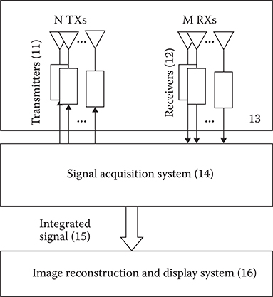
FIGURE 15.1
The general block diagram of a UWB radar system showing the antenna array (13), SAS (14), and image reconstruction and display system (16). The SAS uses analog and digital integration of multiple received signals from the same range (range cell) to increase the SNR of the returns and to compensate for the wide dynamic range of the radar. (Adapted from Gazelle, D. et al., Signal Acquisition System and Method for Ultra-Wideband (UWB) Radar, U.S. Patent No. 7,773,031 B2, August 10, 2010.)
15.3.3 SAS SNR Improvement
Under normal radar conditions, the received SNR decreases with target range because of the increased 1/r 4 attenuation. Integrating a signal for N cycles amplifies the signal by a factor N and the noise root-mean-square (RMS) amplitude by a factor of . Thus we may improve the SNR by integrating the signal over multiple cycles to compensate for all the system losses. When properly configured with multiple channels, the SAS can take signals from many receivers, integrate them, and control the signal acquisition process.
Signals from all receivers for each transmitter integrated in the SAS (15) pass to an image reconstruction and display system (16). Image reconstruction methods can use many different appropriate techniques such as ellipsoidal back-projection. Although many radar systems provide integration by way of digital sampling, the Camero, Inc., SAS samples the received signal on a uniform grid over the time domain at a given Nyquist criterion sampling rate and converts it to discrete digital samples. To achieve the required SNR, the SAS repeats sampling of the return signal at a given instant and performs an analog integration followed by digital integration using well-known digital signal techniques.
The frame rate of real-time radar imaging or other critical radar systems determines the signal acquisition period. This means the imaging frame duration sets the completion time for signal acquisition. During the frame period, the number of transmission/reception cycles (maximum integration number) required for integration must not exceed the total number of transmitted pulses within the frame duration defined by the pulse repetition frequency (PRF) and the number of transmitters N. In many cases, we cannot achieve a required SNR with this maximal integration number.
To get around the maximal integration number constraint, parallel sampling can be performed that samples the received signal on different L > 1 instants. This approach will shorten the additional signal acquisition time by a factor L. This parallelism requires each receive channel to have a very fast ADC sampler with enough bits to fit the required dynamic range and fast electronics to transfer the samples from the many ADCs. This can involve high hardware expenses and power consumption.
15.3.4 Designing the Camero, Inc., SAS
Considering the problems and objectives described above, the engineers needed to find a way to decrease the requirement for dynamic range and the speeds of the ADCs and other digital electronics. The Camero, Inc., SAS has broad applications outside the UWB radar shown in Figure 15.1 and may find applications in other UWB radars. Note how a synthetic aperture radar would provide the equivalent of the multiple transmitters and receivers shown here.
After reviewing the problems and literature of conventional radar signal acquisition methods, the sampling and digitizing configuration was devised (20) (Figure 15.2). The SAS includes a UWB sampler block (21) coupled to an analog integration block (22) coupled through an ADC (23) to a digital integration block (24) Typically, each separate acquisition channel (20) contains the same components and connects to a particular receiver.
To explain the Camero, Inc., SAS operation as shown in Figure 15.2 (20), consider the case of static targets moving slowly compared with the shortest transmitted wavelength during a frame interval. In this case, the periodic received signal is r(t) with a period T = 1/PRF, where PRF indicates the transmission pulse repetition frequency. The sampler block (21) repeatedly samples the received signal r(t) by tuning the sampling instants to the range cells at time t = T0 + nΔT. The nth sampling phase corresponds to the target range nΔTc/2 (where c is the speed of light in vacuum; ΔT is the sampling interval; T0 corresponds to the time of transmission of short UWB pulse by a selected transmitter in the current transmit/receive cycle and the factor 2 accounts for the round trip of the scattered wave).

FIGURE 15.2
Block diagram of one channel of the Camero, Inc., SAS showing the digitizing and integrating elements, which build the signal return from each range cell from the transmitter Txn and receiver Rxm pair. (Adapted from Gazelle, D. et al., Signal Acquisition System and Method for Ultra-Wideband (UWB) Radar, U.S. Patent No. 7,773,031 B2, August 10, 2010.)
The sampled signal goes to the analog integration block (22), which requires a reset at the beginning of each range cell. The sampling and analog integration process repeats for the desired number cycles as described later.
The analog integrator (22) output goes to the ADC (23) for conversion into a digital sample. The stream of digital samples Sn corresponds to the integrated received signal at the nth range cell, which then goes to the digital integration block (24) for further integration by means of discrete time signal processing. The Camero, Inc. SAS has a unique feature because of the following:
The analog integration block configuration compensates for at least part of the signal losses
The digital integration block configuration can substantially compensate for the nominal free space propagation losses
There are several ways to approach the problems of compensation for known/expected losses. For example, in different implementations
The configuration of the analog integration block can substantially compensate for the nominal free space propagation and the digital integration block can compensate for factors such as obstacle-oriented losses, RCS variations
The analog integration block may compensate for obstacle-oriented losses and/or expected RCS variations
The analog integration may partially compensate for propagation losses, and the digital integration block may complete the desired compensation for signal losses
The Camero, Inc., SAS has provisions for a variable number of integration cycles in accordance with the following:
Range (based on reception time)
Desired SNR profile providing better values of SNR for different range cells for a given RCS
Signal loss compensation
For example, to achieve a range-independent SNR for a predefined target RCS, the near range cells will receive a smaller number of integration cycles compared with far ones. In another case, the SAS can maximize the SNR for a subrange of special interest within the constraints of overall integration time, by setting the number of integration cycles for corresponding range cells on account of the integration of other range cells.
The SAS has great flexibility and can use different integration plans to cover any kind of predefined relationship between a number of integration cycles and range/reception time (range cell index). For example, the SAS can be programmed to a desired SNR profile and/or desired compensation for signal losses.
The total SAS may include a database (25) and processor (26) coupled with a digital integration block (24) and/or the analog integration block (22), which is coupled to each receiver channel Rxm. This feature lets the user integrate the database and processor with one or more blocks of the SAS (e.g., with the digital integration block). For example, the database may have precalculated integration plans(s) for a range independent SNR profile or a maximized SNR for selectable subranges, and so on.
15.3.5 Camero, Inc., SAS Calculation of Integration Cycles
By applying some previous information, the number of integration cycles can be calculated based on a known dependence between the nominal propagation path loss and target range/reception time. Some variations on this idea include the following:
Programming precalculated numbers of integrated cycles required for compensation of other types of signal losses such as those caused by a predefined obstacle or expected loss. This would let the operator adjust the processing for looking through different types of construction in through-wall radars based on expected losses.
Programming the SAS to calculate the required numbers of integration cycles with the help of adaptive and/or learning algorithms. This requires having some external interface (27) to obtain data from an image reconstruction system, user, and so on. The adaptive/learning algorithms may complement the precalculated integration plan(s) by enabling path loss compensation in real conditions (e.g., airborne radars) or replacing (partly or fully) the precalculated integration plan(s) by providing on-demand and/or online calculations of the required integration.
The number of integration cycles N required to increase the SNR from some initial value SNR0 to a target value SNRt can be determined by the following equation with SNR values
in dB:
A well-known radar equation found in A. Ishimaru’s Electromagnetic Wave Propagation, Radiation and Scattering [4] states that for a given fixed RCS target, the received SNR depends on the reception time t as follows:
where SNR(t) indicates the SNR at the starting receive time t0.
Equations 15.1 and 15.2 were used to devise an integration plan with the required SNR as a function of the receiving range (SNR profile). For example, an integration plan for a range independent SNR profile for a fixed RCS target is defined as
In this case, N(t) indicates the required number of integration cycles for different range cells as a function of reception time. N0 gives the number of integration cycles for t = t0 given by N0 = 10[SNR t ~SNR(t°)]/1°.
This plan compensates for free space propagation losses and gives a range-independent SNR profile. The Camero, Inc., SAS was designed such that it can predefine and store this integration plan in the system database. Depending on the particular radar antenna array geometry, the SAS may require an individual integration plan for each transmitter/receiver pair. For special cases where the antenna aperture has larger dimensions than the range, all receivers can use the same integration plan. A nonlimiting general example can show the case of an integration plan with a range-independent SNR profile. From Equation 15.3, the signal and noise can be described as the following functions of reception time (or range):
In this situation, the received signal amplitude ν for a given RCS without noise is proportional to v(t) ∝ v0(t0/t)2. This means that the received power varies inversely as range (ct/2)4 or t4, so the amplitude [square root of power] becomes inversely proportional to t2. Therefore, the signal amplitude vis and RMS noise amplitude viN at the integrator output working according to the integration plan of Equation 15.3 would give
where νΝrms describes the additive white noise RMS amplitude.
Thus Equation 15.5 shows how to achieve a constant SNR and an integrated signal (and noise) level that increases with range. Implementing the plan with only an analog integrator requires large number of bits to cope with the extended signal dynamic range at the ADC input. As shown in Figure 15.1, there is a similar problem when building an integration plan with only a digital integrator. To solve these problems, the Camero, Inc., SAS splits the integration process into two parts: analog integration followed by digital integration. This approach gives us an additional degree of freedom because we can design it for two separate integrators according to different criteria. For example, we can minimize the signal dynamic range of the ADC to reduce costs and get an adequate SNR at the output of the digital integrator.
The Camero, Inc., SAS can split the overall number of integration cycles N(t) into Na(t) analog integration cycles and Nd(t) digital integration cycles so Na(t) × Nd (t) = N(t). Given this, if , then we get the received signal amplitude at the output of the analog integration block as . According to this proposed integration plan, the received signal from a given RCS target becomes range independent after the analog integration. This compensates for the free space path loss and minimizes the expected signal dynamic range at the input of the ADC port. For example, this can reduce the ADC dynamic range requirements from 86 to 110 dB, as described in Figure 15.1, to less than 50 dB for some environments, where the obstacle caused variations contribute to 30 dB losses and target RCS diversity contributes to 20 dB losses.
Some versions of the Camero, Inc., SAS may perform the analog-to-digital conversion of the analog integrator output once, for each period of analog integration as shown in Figure 15.3. This will considerably reduce the required ADC conversion rate for integration plans with the number of analog integrations strictly greater than 1. This helps the SAS to use relatively low-cost slow ADCs. The SAS can reduce the signal acquisition power consumption that depends on the ADC conversion rate. Those familiar with signal processing would know that many variations exist for the equivalent and/or modified functionality of the SAS.

FIGURE 15.3
The Camero, Inc., SAS block diagram. This shows the operations performed on each frame including the analog conversion and digital integration of signals from each range cell. The number of analog and digital integrations may vary according to the time increment t0,t1, . . . ,tn to give an optimal SNR for targets at all ranges. (Adapted from Gazelle, D. et al., Signal Acquisition System and Method for Ultra-Wideband (UWB) Radar, U.S. Patent No. 7,773,031 B2, August 10, 2010.)
15.3.6 Alternate Signal Integration Methods
The Camero, Inc., SAS can have many implementations, but the following examples show some basic approaches: (1) off-line a priori information plan; (2) interactive user integration and noise plan; (3) automatic adaptive plan; and (4) online automatic predefined adaptive integration plan. The patent covers all variations of these.
Off-line a priori information plan: This off-line plan assumes a priori known system operation information about fixed losses and/or noise sources and takes this into account during the system design phase or in preparation for a specific use. We can summarize the a priori information by the following:
where SNR(t) describes the expected SNR versus reception time (or range) given by the a priori known function F1(t); P(t) is the expected received power at reception time t (corresponding to a target of given RCS located at range ct/2); and FR is the required imaging frame rate. We can supply F1(t) and F2(t) with a table or a mathematical representation such as the one shown in Equation 15.2 (i.e., SNR(t) = SNR(t0) - 40 × log10(t/t0), [dB]). Generally F1(t) depends on F2(t) because the received SNR depends on the received power and the receiver frontend additive noise profile F1(t) = F2(t)/Pnoise(t), where Pnoise(t) is the additive noise power profile (which typically comes from thermal sources at the frontend and has a profile Pnoise(t) = const). The plan may require additional information for calculating the integration plan as shown in Table 15.1.
We can then calculate the required analog, Na(t), and digital, Nd(t), integrations from
where N(t) is the total integration plan (according to the required integrated SNR profile) given by
TABLE 15.1
Camero, Inc., SAS Off-Line A Priori InformationRequired Information Symbol Function/Description Source SNR profile goal SNRt(t) Required integrated SNR vs. reception time (or range) Given ADC limit Vmax(ADC) Maximum admissible ADC input voltage (ADC saturation power) ADC specifications Frontend gain AFE Gain between antenna and ADC with no integration Measured Characteristic impedance Z0 Frontend characteristic impedance Measured Pulse repetition rate PRR System transmission PRR Design specifications which is subject to the constraint
This constraint ensures that the total number of cycles used to acquire the signal does not exceed the number of transmitted pulses in the frame duration. We can increase the system PRF or decrease the imaging frame rate FR to satisfy the constraint.
This Camero, Inc., SAS off-line a priori integration plan may provide a better utilization of ADC bits and give an integrated signal with the desired SNR profile SNRt(t). Note that because the equations for Na(t) and Nd(t) have integer values, we must round results of calculations to the closest integer, subject to Na(t), Nd(t) > 1. The calculation should include at least one cycle of integration for each range cell, otherwise it makes the radar equivalent to one with no processing.
Interactive user integration and noise plan: This plan will have a user interface that permits adjusting the number of analog integrations Na(t) and digital integrations Nd(t). The operator can interactively recognize a subrange with poor imaging or detection performance and change the integration plan by using more transmission cycles to integrate the signal at this subrange.
Automatic adaptive plan: This plan uses special purpose algorithms capable of analyzing the quality of integrated received signals and/or reconstructed images to adjust the system to achieve predefined goals. This might work by including a processor/database to collect statistics about the integrated signal power versus range. By analyzing these statistics we might recognize an abrupt decrease in signal power at some range (corresponding to a reception time denoted by t’) in the mean received power and related to an obstacle at the corresponding range. The processor can then increase Na(t) for t > t’ to remove the discontinuity. In this case, Equation 15.8 (for Nd(t)) will determine Na(t) and Nd(t) within the constraint of Equation 15.10 (i.e., Σ N(t) < PRF/FR).
Online automatic predefined adaptive integration plan: This plan uses special purpose algorithms, which use feedback from integrated received signals and/or reconstructed image to modify the integration plan to achieve a predefined goal. For example, as the system operates, the processor/database may collect statistics about the integrated received power versus range. These statistics could indicate an abrupt decrease or discontinuity in the mean received signal power at some range corresponding to reception time t’, indicating the presence of an obstacle at that range. The processor may use these algorithms to increase Na(t) for t > t and cause the discontinuity to vanish. Again Na(t) and Nd(t) are related through Equation 15.8, Nd(t) = N(t)/Na(t), and fulfill the constraint of Equation 15.10.
15.3.7 The Camero, Inc., SAS General Operating Principles
Figure 15.3 shows a generalized operating diagram of how the Camero, Inc., SAS works in accordance with some of the embodiments described earlier. During operation the SAS captures a signal from each of the n transmitters (TX1,TX2, . . . , TXN) sequentially during a frame (31). This means each transmitter acquires the received signals (32) for the entire range. The SAS takes the different simultaneous sampled range cells (t0, t1, etc.) for all m receivers (RX1,RX2, . . . , RXM) and performs Na analog and Nd digital integrations on each analog integrated sample. As mentioned earlier, the number of analog and digital integrations for each range cell can vary according to a priori assumptions about the range, or as required, based on image analysis or operator adjustment. The system resets the analog integrators (typically one per receiver) prior to each integration section. In Figure 15.3, r1/M (t3) and r1M (ti) stand for the integrated sample corresponding to the received signal at receiver M at times t3 and t, respectively, received from the reflected signal from transmitter TX1. As shown in the figure of the integration plan example, the number of integration cycles (Nd, Na, etc.) differs for different range cells.
We can imagine other signal acquisition schemes capturing the frame sequentially, range cell after range cell (in an increasing order), so that each range cell runs sequentially over all transmitters.
The Camero, Inc., SAS may take the form of a suitably programmed computer, or a computer program, or a machine-readable memory embodying a program of instruction to perform the functions described here.
15.4 Conclusions
The patented Camero, Inc., SAS takes a new approach to correcting the problem of increasing SNR as range weakens the return signal. Using multiple analog and digital integrations for each range cell opens possibilities for improving the performance of all radar systems. This allows the signal processing or imaging system to have an optimal SNR at all ranges. The Camero, Inc., Xaver™400 and Xaver™800 series use a combination of the SAS and time delay calibration system (TDCS) described in Chapter 16 to achieve high-quality real-time imaging performance shown in Chapter 11.
References
1. Gazelle, D., Beeri, D., and Daisy, R., Signal Acquisition System and Method for Ultra-Wideband (UWB) Radar, U.S. Patent No. 7,773,031 B2, August 10, 2010.
2. Shima, A., Fujisaka, T., and Ohashi, Y., Pulsed Doppler Radar System having an Improved Detection Probability, U.S. Patent No. 5,132,688, July 1992.
3. Mitsumoto, M., Sugimoto, T., Fujisaka, T., and Kondo, M., Radar Signal Processor and Pulse Doppler Radar System Therewith, U.S. Patent No. 5,457,462, October 1995.
4. Ishimaru, A., Electromagnetic Wave Propagation, Radiation and Scattering, Prentice Hall: Englewood Cliffs, NJ, 1990.
5. Wolff, C., Radar Tutorial. Radar receivers. Online: http://www.radartutorial.eu/09.receivers/rx04.en.html