CHAPTER 5

Reliability and Scalability Methods

CONTENTS

5.0 Introduction to High-Availability Systems

5.0.1 Reliability Metrics

5.0.2 Detection and Repair of Faults

5.0.3 Failure Mechanisms

5.1 HDD Reliability Metrics

5.1.1 Failure Rate Analysis Domains

5.2 Methods for High-Availability Design

5.2.1 RAID Arrays

5.2.2 RAID Level Defi nitions

5.2.3 RAID Clusters

5.3 Architectural Concepts for HA

5.3.1 Single Point of Failure

5.3.2 No Single Point of Failure

5.3.3 N + 1 Sparing

5.3.4 Networking with High Availability

5.3.5 Mirroring Methods

5.3.6 Replication of Storage

5.3.7 Client Caching Buys Time

5.3.8 Other Topologies for HA

5.3.9 Concealment Methods

5.3.10 A Few Caveats

5.4 Scaling and Upgrading System Components

5.4.1 Upgrading Components

5.5 It’s a Wrap—Some Final Words

References

5.0 INTRODUCTION TO HIGH-AVAILABILITY SYSTEMS

Things do not always go from bad to worse, but you cannot count on it. When money is on the line, system uptime is vital. A media services company charges clients $1K/day for editing and compositing services. A broadcaster is contracted to air the Super Bowl or World Cup finals along with $100M worth of commercials. A home shopping channel sells $10K worth of products per hour from on-air promotions. It is very easy to equate lost revenue to reliable equipment operations. How much time and money can you afford to lose in the event of downtime? Reliability is a business decision and must be funded on this basis. Therefore, it is straightforward to calculate the degree of reliability (and money to realize it) needed to secure continuous operations. For this reason, A/V facility operators often demand nearly 100 percent uptime for their equipment.

Of course, getting exactly 100 percent guaranteed uptime is impossible no matter how meticulous the operations and regardless of what backup equipment is available. Getting close to 100 percent is another matter. The classic “six sigma” measure is equivalent to 3.4 parts per million or an uptime of 99.9997 percent. In 1 year (8,760 hr), this equates to about 1.5 min of downtime. Adding another 9 results in 9.5 s of total downtime per year. In fact, some vendors estimate that adding a 9 may cost as much as a factor of 10 in equipment costs at the 99.999 percent level for some systems. Adding nines is costly for sure. This chapter investigates the techniques commonly used to achieve the nines required to support high-availability A/V systems. Also, it examines methods to scale systems in data rate, storage, and nodes.

5.0.1 Reliability Metrics

The well-known mean or average time between failures (MTBF) and mean time to repair (MTTR) are the most commonly used metrics for predicting up- and downtime of equipment. MTBF is not the same as equipment lifetime. A video server may have a useful life of 7 years, yet its MTBF may be much less, just as with a car, boat, or other product. An even more important metric is system availability (Av). How do MTBF and MTTR relate to availability?

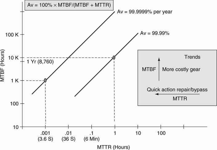
Let us consider an example. If the MTBF (uptime) for a video server is 10,000 hr and the MTTR (downtime) is 1 hr, then the server is not usable for 1 hr every 1.15 y on average. (Because Av—uptime/(uptime downtime)* 100 percent, then Av—99.99 percent availability for this example.) As MTTR increases, the availability is reduced. However, if the MTBF is small (1,000 hr) and if the MTTR is also small (3.6 s, auto failover methods), then Av may be excellent—99.9999 percent for this case. MTTR is an important metric when computing Av and for achieving highly available systems.

Figure 5.1 illustrates how availability is related to MTBF and MTTR. There are two significant trends. One is as MTBF is raised, the cost of equipment/systems usually raises too. Makes sense: more reliable gear requires better components, design, and testing. However, excellent Av can be maintained even with inexpensive gear if the MTTR is reduced correspondingly. A design can trade off equipment cost against quick repair/reroute techniques and still achieve the desired Av. It is wise to keep this in mind when selecting equipment and system design styles. Even inexpensive gear has the potential of offering excellent Av if it can be replaced or bypassed quickly. Incidentally, for most TV channels, a MTTR of less than ~ 10 s for the main broadcast signal is crucial to prevent viewers from switching away.

FIGURE 5.1 System device availability versus MTBF and MTTR.

Sometimes the term fault-tolerant system is used to describe high availability. (Well, nothing is completely fault tolerant with an Av—100 percent.) In most so-called fault-tolerant systems, one (or more) component failure can occur without affecting normal operations. However, whenever a device fails, the system is vulnerable to complete failure if additional components fail during the MTTR time.

One example of this is the braking system in a car. Many cars have a dual-braking, fault-tolerant system such that either hydraulic circuit can suffer a complete breakdown and the passengers are in no danger. Now, if the faulty circuit is not repaired in a timely manner (MTTR) and the second braking system fails, then the occupants are immediately in jeopardy.

This analogy may be applied to an A/V system that offers “fault tolerance.” In practice, sometimes a single system component fails, but no one replaces the bad unit. Due to poor failure reporting alarms or inadequate staff training, some single failures go unnoticed until a second component fails months or even years later—“Hey, why are we off the air?” Next, someone is called into the front office to explain why the fault-tolerant system failed.

5.0.2 Detection and Repair of Faults

Figure 5.2 shows a typical fault diagnosis and repair flow for a system with many components. There are two independent flows in the diagram: automated and manually based. Of course, all systems support manual repair, but some also support automatic self-healing. Let us focus on the automated path first on the left side of Figure 5.2. Automatic detection of a faulty component/path triggers the repair process. Detection may include HDDs, servers, switch ports, A/V links, and so on. Once the detection is made, then either self-healing occurs or a manual repair is required. Ideally, the system is self-healing and the faulty component is bypassed (implying alternate paths) or repaired in some automatic yet temporary way. The detection and repair should be transparent to the user community. In a traditional non-mission-critical IT environment, self-healing may take seconds to a minute(s) with few user complaints.

FIGURE 5.2 Failure detection and repair process flow in an A/V system.

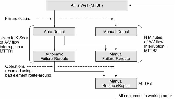
For many A/V applications, self-healing needs to be instantaneous or at least appear that way. Ideally, under a single component failure, no A/V flow glitching occurs. Quick failover is an art and not easy to design or test for. If done well, automated detection and healing occur in “zero” seconds (MTTR1 in Figure 5.2). In reality, most self-healing A/V systems can recover in a matter of a second or so. With proper A/V buffering along the way, the failure has no visual or user interface impact.

A no single point of failure (NSPOF) design allows for any one component to fail without operations interruption. Very few systems allow for multiple simultaneous failures without at least some performance hit. The economic cost to support two, three, or four crucial components failing without user impact goes up exponentially.

With an SPOF design, a crucial component will cause A/V interruption for a time MTTR2. Even with the automatic detection of an anomaly, the manual repair path must be taken as in Figure 5.2. Usually, MTTR2 is much greater than MTTR1. This can take seconds if someone is monitoring the A/V flow actively and is able to route around the failed component quickly. For example, Master Control operators in TV stations or playout control rooms are tasked to make quick decisions to bypass failed components. In other cases without a quick human response, MTTR2 may be minutes or even days. It should be apparent that availability (Av) is a strong function of MTTR. SPOF designs are used when the economic cost of some downtime is acceptable. Many broadcasters, network originators, and live event producers rely on NSPOF designs in the crucial paths at least.

The worst-case scenario is the right side flow of Figure 5.2. Without automatic detection, it often takes someone to notice the problem. There are stories of TV channel viewers calling the station to complain of image-quality problems unnoticed by station personnel. Once failure is detected, the active signal path must be routed to bypass the faulty component. Next, the faulty part should be replaced/repaired (MTTR3). All this takes time, and MTTR2 + MTTR3 can easily stretch into days.

In either case, manual or automatic detection, the faulty component eventually needs to be repaired or replaced. During this time, a NSPOF system is reduced to a SPOF one and is vulnerable to additional component failure. As a result, MTTR3 should be kept to a minimum with a diligent maintenance program. Examples of these system types are presented later in the chapter. The more you know about a system’s health, the quicker a repair can be made. covers monitoring and diagnostics—crucial steps in keeping the system availability high.

5.0.3 Failure Mechanisms

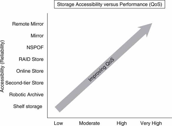
In general, A/V systems range from small SPOF types to full mirror systems with off-site recovery. Figure 5.3 plots the available system performance versus the degree of availability for storage components. Similar plots can be made for other system-level elements. Levels of reliability come in many flavors, from simple bit error correction to the wholesale remote mirroring of all online data. The increasing performance metric is qualitative but indicates a greater QoS in accessibility, reduced access latency, and speed.

FIGURE 5.3 Storage accessibility versus performance (QoS).

Individual devices such as archives, servers, switches, near-line storage, or A/V components each have a MTBF metric. Common system elements and influences (not strictly prioritized in the following list) that can contribute to faults are

In general, the three most common failure sources are human operational error and software- and hardware-related faults. Depending on the system configuration, either of these may dominate as failure modes. For non-human-related faults, Horison Information Strategies estimates that, on average, hardware accounts for 38 percent of faults, 23 percent is network based (including operational failures), 18 percent is software related, and 21 percent other.

Elements and influences are often interrelated, and complex relationships (protocol states) may exist between them. Device hardware MTBF may theoretically be computed based on the underlying design. Although in practice, it is difficult to calculate and is known more accurately after measuring the number of actual faulty units from a population over a period of time. A device’s software MTBF is almost impossible to compute at product release time, and users/buyers should have some knowledge of the track record of a product or the company’s reputation on quality before purchase. Often a recommendation from a trusted colleague who has experience with a product or its vendor is the best measure of quality and reliability.

In the list given earlier, the upper half items are roughly the responsibility of the supplying vendor(s) and system’s integrator, whereas the lower half items are the responsibility of the user/owner. Much finger pointing can occur when the bottom half factors are at fault but the upper half factors are blamed for a failure. When defining a system, make sure that the all modes of operation are well tested by the providing vendor(s).

Naturally, one of the most common causes of failure is the individual system element. Figure 5.4 shows a typical internal configuration for a device with multiple internal points of failure. It is very difficult to design a stand-alone “box” to be fault tolerant. For most designs, this would require a duplication of most internal elements. This is cost prohibitive for many cases and adds complexity. In general, it is better to design for single unit failure with hot spares and other methods to be described. That being said, it is good practice to include at least some internal-redundant elements as budget permits.

FIGURE 5.4 Standalone device with potential internal failure points.

The most likely internal components to fail are mechanically related: fans, connectors, HDD, and structure. The power supply is also vulnerable. Cooling is often designed to withstand at least one fan failure, and it is common to include a second power supply to share the load or as a hot spare. The most difficult aspect to duplicate is the main controller if there is one. With its internal memory and states of operations, seamlessly failing over to a second controller is tricky business.

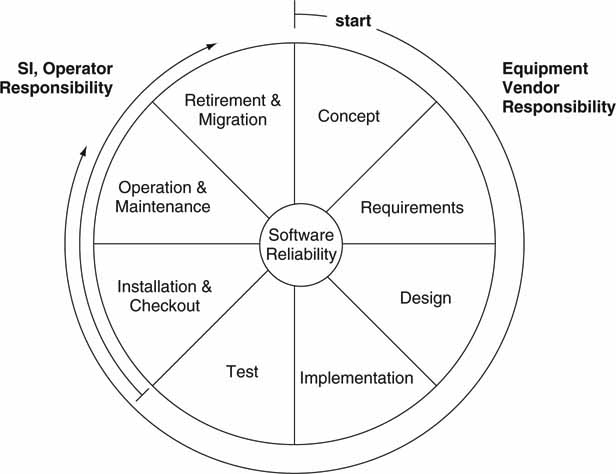
Ah, then there is software reliability. This is without a doubt the most difficult aspect of any large system. Software will fail and users must live with this fact and design systems with this in mind. The software life cycle is shown in Figure 5.5. From concept to retirement/migration, each of the eight steps should include software design/test methodologies that result in reliable code. Note that some steps are the responsibility of the original equipment vendor, whereas others belong to the operator or installer/SI.

FIGURE 5.5 Software reliability and its life cycle.

In the classic work The Mythical Man-Month, a surprising conclusion was learned from designing software for the IBM 360 mainframe: in complex systems the total number of bugs will not decrease over time, despite the best efforts of programmers. As they fix one problem or add new features, they create another problem in some unexpected way.

There are ways to reduce this condition, but bugs will never go to zero. The good news is that software does not make mistakes, and it does not wear out. See more on Lehman’s laws of software evolution in Chapter 4.

One hot topic is software security in the age of viruses, worms, denial of service attacks, and so on. Although a security breach is not a failure mechanism in the traditional sense, the results can be even more devastating. Traditional A/V systems never contended with network security issues, but IT-based systems must. Of course, A/V systems must run in real time, and virus checkers and other preventative measures can swamp a client or server CPU at the worst possible moment with resulting A/V glitches or worse. It takes careful design to assure system integrity against attacks and to keep all real-time processes running smoothly. One key idea is to reduce the surface of attack. When all holes are closed and exposure to foreign attacks is limited, systems are less vulnerable. This and other security-related concepts are covered in more detail in Chapter 8.

A potential cause of performance degradation—a failure by some accounting—is improper use of networked-attached A/V workstations. For example, a user may be told not to initiate file transfers from a certain station. If the advice is ignored, the network may become swamped with data, and other user’s data are denied their rightful throughput. This is a case of a fault caused by user error.

Before starting the general discussion of configurations for high availability, let us investigate how reliability is measured for one of the most valuable elements in an A/V design: the hard disk drive.

5.1 HDD RELIABILITY METRICS

Because disk drives are core technology in networked media systems, it is of value to understand how drive manufacturers spec reliability. Disk drive manufacturers often state some amazing failure rates for their drives. For example, one popular SCSI HDD sports a MTBF of 1.2 million hours, which is equivalent to 137 years. The annual failure rate (AFR) is 0.73 percent. How should these values be interpreted? Does this mean that a typical HDD will last 137 years? It sounds ridiculous; would you believe it? What do MTBF and AFR really mean? The following sections investigate these questions. First, let us classify failure rate measurements into three different domains.

5.1.1 Failure Rate Analysis Domains

Measuring HDD failure rate is a little like the proverbial blind man describing an elephant—depending on his viewing perspective, the elephant looks quite a bit different. The three domains of HDD failure rate relevance are (1) lab test domain, (2) field failure domain, and (3) financial domain.

5.1.1.1 Lab Test Domain

The lab test domain is a well-controlled environment where product engineers simultaneously test 500–1,000 same-vintage drives under known conditions: temperature, altitude, spindle on/off duty cycle, and drive stress R/W conditions. In this domain there are various accepted methods to measure HDD failure rates. The International Disk Drive Equipment and Materials Association (IDEMA, www.idema.org) sets specs that most HDD manufacturers adhere to. The R2-98 spec describes a method that blocks reliability measurements into four periods. The intervals are 1–3 months, 4–6 months, 7–12 months, and 13 to end-of-design-life. In each period the failure rate expressed as X %/1,000 hours is measured. In reality, the period from 1 to 3 months is the most interesting. The results of these tests are not normally available on a drive spec sheet because evaluating a multivariable reliability metric is a knotty problem and may complicate a buyer’s purchase decision.

Many electrical/mechanical components have a failure rate that is described by the bathtub curve as shown in Figure 5.6. A big percentage of “infant mortality” failures normally occur within the first 6 weeks of an HDD usage. If vendors exercise their product (burn-in) during these early weeks before shipment, the overall field failure rate decreases considerably. However, most cannot afford to run a burn-in cycle for more than a day or two, so failure rates in the field are dominated by those from the early part of the curve. In fact, most HDD vendors test SCSI drives 24/7 for 3 months during the design phase only. Correspondingly, ATA drives are often tested using stop/start and thermal cycling. This is yet another reason why SCSI is more costly than ATA drives.

FIGURE 5.6 Component failure rate over time.

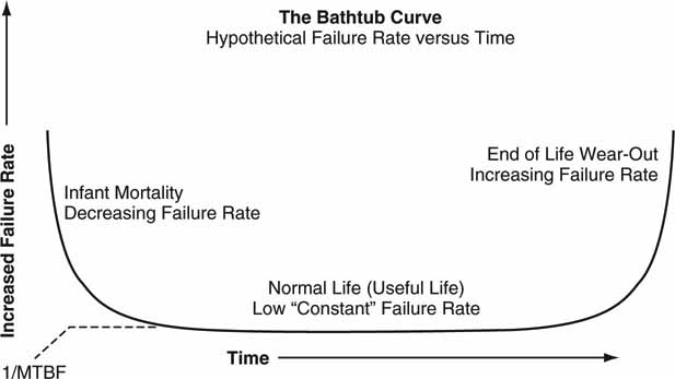
However, about 10 times more ATA disk drives are manufactured today than SCSI and Fibre Channel drives combined. At these levels, ATA drive manufacturers are forced to meet very high process reliability requirements or else face extensive penalties for returned drives.

The IDEMA also publishes spec R3-98, which documents a single X%/1,000 hours failure rate metric. For this test, a manufacturer measures a collection of same-vintage drives for only 3 months of usage. For example, if an aggregate failure rate was measured to be 0.2%/1,000 hours, we may extrapolate this value and expect an HDD failure before 500,000 hours (100/0.2 *1,000) with almost 100 percent certainty. However, the R3-98 spec discourages using MTBF in favor of failure rate expressed as X%/1,000 hours over a short measurement period. Nonetheless, back to the main question, how should MTBF be interpreted?

Used correctly, MTBF is better understood in relation to the useful service life of a drive. The service life is the point where failures increase noticeably. Drive MTBF applies to the aggregate measurement of a large number of drives, not to a single drive. If a drive has a specified MTBF of 500,000 hours (57 years), then a collection of identical drives will run for 500,000 device hours before a failure of one drive occurs. A test of this nature can be done using 500 drives running for 1,000 hours. Another way of looking at drive MTBF is this: run a single drive for 5 years (service life, see later) and replace it every 5 years with an identical drive and so on. In theory, a drive will not fail before 57 years on average.

5.1.1.2 Field Failure Domain

Next, let us consider failure rate as derived from units returned from the field—the field failure domain. In this case, manufacturers measure the number of failed and returned units (normally under warranty) versus the number shipped for 1 year. The annual return rate or annual failure rate may be calculated from these real-world failures. Of course, the “test” conditions are almost completely unknown, with some units being in harsh environments and others rarely turned on. The return rate of bad drives is usually lower than the actual respective failure rate. Why? Some users do not return bad drives and some drives stay dormant on distributors’ shelves. So this metric is interesting but not sufficient to predict a drive’s failure rate.

5.1.1.3 Financial Domain

The final domain of interest is what will be called the financial domain. The most useful statistic with regard to HDD reliability is the manufacturer’s warranty period. The warranty period is the only metric that has a financial impact on the manufacturer. Most vendors spec only a 5-year warranty—nowhere close to the 100+ years that the MTBF data sheet value may imply. For practical purposes, let us call this the service life of the drive. Of course the HDD manufacturer does not expect the drive to fail at 5 years and 1 day. Also, typical warranty costs for an HDD manufacturer are about 1 percent of yearly revenue. Because this value directly affects bottom-line profits, it is in the manufacturer’s best interest to keep returns as a very small percentage of revenue.

In reality, the actual drive lifetime is beyond the 5-year warranty period but considerably short of the so-called MTBF value. Conservatively built systems should be biased heavily toward the warranty period side of the two extremes. Of course, HDD reliability is only one small aspect of total system reliability. However, understanding these issues provides valuable insights for estimating overall system reliability and maintenance costs.

5.2 METHODS FOR HIGH-AVAILABILITY DESIGN

There are two kinds of equipment and infrastructure problems: those you know about and those you don’t. The ones you don’t know about are the most insidious. They hide and wait to express themselves at the worst time. Of those you know about, some can be repaired (corrected) and some can’t. So, in summary, problems can be classified as follows:

Here are some simple examples of these four:

The set of four examples deals with bad bits. Other error types occur, such as failed hardware components, broken links, software bugs. Each error type may need a custom error detection scheme and/or associated error correction method. It is beyond the scope of this book to analyze every possible technique. Nonetheless, keep these high-level concepts in mind as this chapter develops various methods for creating reliable systems out of inherently unreliable devices.

The high-availability (HA) systems’ methods under discussion are RAID for storage, storage clusters, NSPOF, N + 1 sparing, dual operations, replication, mirroring, and disaster recovery.

5.2.1 RAID Arrays

The RAID [redundant arrays of inexpensive (independent, nowadays) disks] concept was invented at UC Berkeley in 1987. Patterson, Gibson, and Katz published a paper titled “A Case for Redundant Arrays of Inexpensive Disks (RAID).” This paper described various types of disk array configurations for offering better performance and reliability. Until then, the single disk was the rule, and arrays were just starting to gain acceptance. The authors developed seven levels of RAID. Before we define each technique formally, let us illustrate how RAID works in general terms.

The basic idea behind most RAID configurations is simple. Use a parity bit to correct for one missing (bad) bit out of K bits. Figure 5.7 shows a 6-bit data field and one parity bit. Parity measures the evenness or oddness of the 6-bit string. For example, the sequence 001100 has even parity (P = 0), as there are an even number of ones, whereas the sequence 101010 has odd parity (P = 1). If any single bit is in error, then when the stored parity bit is used, the bad bit may be reconstructed. Parity is generated using the simple XOR function. It is important to note that data bit reconstruction requires knowledge of the bad bit (or data block or array) position. If the 0011 × 0 sequence in Figure 5.7 is given and P = 0 (even number of ones), then it is obvious that X = 0; otherwise, P could not equal zero. Of course, the parity idea can be extended to represent the parity of a byte, word, sector, entire HDD, or even an array. Hence, a faulty or intermittent HDD may be reconstructed. With an array of N data drives and one parity drive, one HDD can be completely dead and the missing data may be recovered completely. Most RAID configurations are designed to reconstruct at least one faulty HDD in real time.

FIGURE 5.7 RAID reconstruction example using parity.

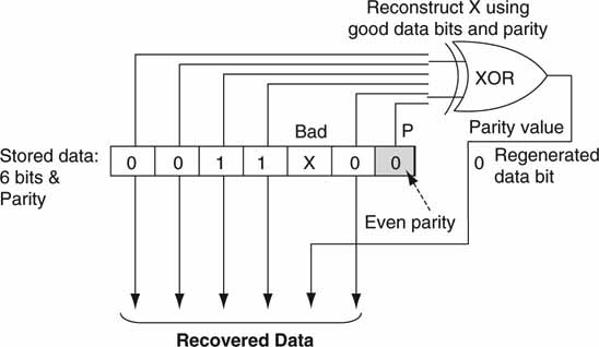
Figure 5.8 is typical of an HDD array with RAID protection. In this case, the disks are protected by two RAID controllers. Either can R/W to a disc or do the needed RAID calculations. In the event of one controller going haywire, the second becomes responsible for all I/O. If designed correctly, with a passive backplane and dual-power supplies, this unit offers NSPOF reliability. Note too that each HDD has a direct link to each controller. A less reliable array may connect each HDD to one or two internal buses. In this case, one faulty HDD can hang a bus and all connected drives will become inaccessible. With care, an array can offer superior reliability. Several manufacturers offer NSPOF, dualcontroller arrays ranging from a small 8-drive enclosure to an enormous array with 1,100 drives.

FIGURE 5.8 HDD array with dual RAID controllers.

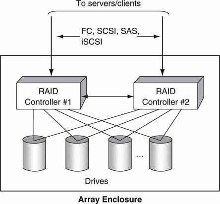
Incidentally, all clients or servers that access the storage array must manage the failover in the event of a controller failing or hanging. For example, if a client is doing a read request via controller #1 but with no response, it is the client’s responsibility to abort the read transaction and retry via controller #2. As may be imagined, the level of testing to guarantee glitch-free failover is nontrivial. This level of failover is offered by a few high-end A/V systems’ vendors.

5.2.1.1 Two-Dimensional (2D) Parity Methods

If we extend the RAID idea, it is possible to design a 2D array with two levels of parity. Figure 5.9 shows a 2D approach. One dimension implements horizontal RAID with parity for correcting data from a single faulty HDD. The second dimension implements vertical RAID and can correct for an entire array in the event of failure. The vertical parity method spans arrays, whereas the horizontal method is confined to a single array. The overhead in vertical parity can be excessive if the number of protected arrays is low. A four (three data VP) array system has 25 percent overhead in vertical parity plus the horizontal parity overhead. Note that the parity value P3 is of no use when the entire array faults. Two-dimensional parity schemes can be complex, and they offer excellent reliability but are short of a complete mirror of all data.

FIGURE 5.9 Two-dimensional horizontal and vertical parity methods.

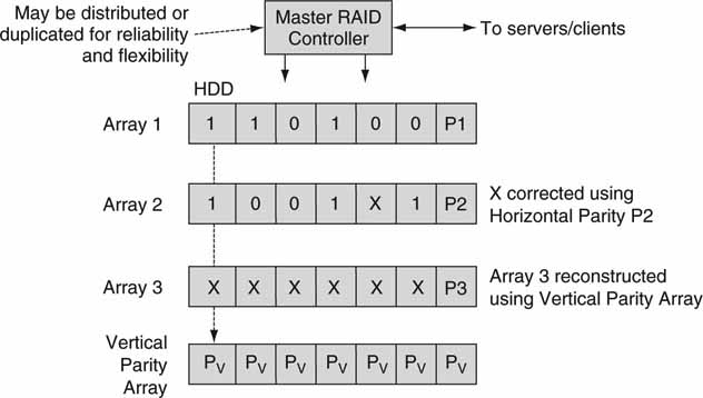
Two-dimensional parity methods require some sort of master RAID controller to manage parity. For standard 1D parity, each array has its own internal (normally, as shown in Figure 5.8) controller(s) for managing the parity values and reconstructing data. However, for a 2D parity method as illustrated in Figure 5.9, no single internal array controller can easily and reliably manage both H and V parity across all arrays. However, there are several different controller configurations for managing and reconstructing missing data using 2D parity. Three of these are as follows:

5.2.1.2 Factors for Evaluating RAID Systems

Despite the relative conceptual simplicity of RAID using parity, here are some factors to be aware of:

5.2.2 RAID Level Definitions

The following sections outline the seven main RAID types. Following this, the RAID levels are compared in relation to the needs of A/V systems.

5.2.2.1 RAID-0

Because RAID level 0 is not a redundancy method, it does not truly fit the “RAID” acronym. At level 0, data blocks are striped (distributed) across N drives, resulting in higher data throughput. See Figure 3A.14 for an illustration of file striping. When a client requests a large block of data from a RAID-0 array, the array controller (or host software RAID controller) returns it by reading from all N drives. No redundant information is stored and performance is very good, but the failure of any disk in the array results in data loss, possibly irrecoverably. As a memory aid, think “RAID-0 means zero reliability improvement.”

5.2.2.2 RAID-1

RAID level 1 provides redundancy by writing all data to two or more drives. The performance of a level 1 array tends to be faster on reads (read from one good disk) and slower on writes (write to two or more disks). This level is commonly referred to as mirroring. Of course, a mirror requires 2 N disks compared to a JBOD (N raw disks), but the logic to manage a mirror is simple compared to other RAID redundancy schemes.

5.2.2.3 RAID-01 and RAID-10 Combos

Both RAID-01 and RAID-10 use a combination of RAID-0 and -1. The 01 form is a “mirror of stripes” (a mirror of a RAID-0 stripe set), and the 10 form is a “stripe of mirrors” (a stripe across a RAID-1 mirror set). There are subtle trade-offs between these two configurations, and performance depends on the distance the mirrors are separated.

5.2.2.4 RAID-2

RAID level 2, which uses Hamming error correction codes, is intended for use with drives that do not have built-in error detection. Because all modern drives support built-in error detection and correction, this level is almost never used.

5.2.2.4 RAID-3

RAID level 3 stripes byte-level data across N drives, with N-drive parity stored on one dedicated drive. Bytes are striped in a circular manner among the N drives. Byte striping requires hardware support for efficient use. The parity information allows recovery from the failure of any single drive. Any R/W operation involves all N drives. Parity must be updated for every write (see Figure 5.10). When many users are writing to the array, there is a parity drive write bottleneck, which hurts performance. The error correction overhead is 100% * [1/N] compared to 100 percent for the mirror case. A RAID-3 set is sometimes referred to as an “N + 1 set,” where N is the data drive count and 1 is the parity drive.

Although not an official RAID level, RAID-30 is a combination of RAID-3 and RAID-0. RAID-30 provides high data transfer rates and excellent reliability. This combination can be achieved by defining two (or more) RAID sets within a single array (or different arrays) and stripe data blocks across the two sets. An array with K total drives may be segmented into two RAID-3 sets, each as N + 1 drives. For example, with K = 10 drives, 4 + 1 and 4 + 1 RAID-3 sets may be defined within a single array. User data may be block striped across the two sets using a RAID-0 layout. Note that any two drives may fail, without data loss, if they are each in a different set.

FIGURE 5.10 RAID level 3 with dedicated parity drive.

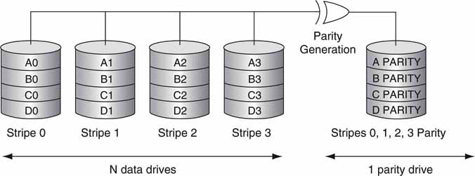
Source: AC&NC.

5.2.2.6 RAID-4

RAID level 4 stripes data at a block level, not byte level, across several drives, with parity stored on one drive. This is very similar to RAID-3 except the striping is block based, not byte based. The parity information allows recovery from the failure of any single drive. The performance approaches RAID-3 when the R/W blocks span all N disks. For small R/W blocks, level 4 has advantages over level 3 because only one data drive needs to be accessed. In practice, this level does not find much commercial use.

5.2.2.7 RAID-5

RAID level 5 is similar to level 4, but distributes parity among the drives (see Figure 5.11). This level avoids the single parity drive bottleneck that may occur with levels 3 and 4 when the activity is biased toward writes. The error correction overhead is the same as for RAID-3 and -4. RAID-50, similar in concept to RAID-30, defines a method that stripes data blocks across two or more RAID-5 sets.

FIGURE 5.11 Raid level 5 with distributed parity.

Source: AC&NC.

5.2.2.8 RAID-6

RAID-6 is essentially an extension of RAID level 5, which allows for additional fault tolerance by using a second independent distributed parity scheme (two-dimensional, row/column computed parity) as illustrated in Figure 5.12. There are several ways to implement this level. In essence, with two parity values, two equations can be solved to find two unknowns. The unknowns are the data records from the two bad drives. This scheme supports two simultaneous drive failures (within a RAID set) without affecting performance (ideally). So, any two drives in Figure 5.12 could fail with no consequent loss of data. This mode is growing very popular, and several IT-and A/V-specific vendors offer storage with this protection level. Compare this to Figure 5.9 where the 2D parity is distributed across several arrays, not only across one array.

FIGURE 5.12 RAID level 6 with 2D parity.

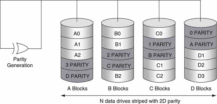
Source: AC&NC.

The salient RAID aspects are as follows:

RAID calculations may be done in the array’s I/O controller or in the attached client. In the first case, dedicated hardware is used to do the RAID calculations, or the RAID logic is performed by software in the CPU on the I/O controller. However, client-based RAID is normally limited to one client, as there is the possibility of conflicts when multiple client devices attempt to manage the RAID arrays. Microsoft supports so-called software RAID in some of its products.

At least one A/V vendor (Harris’s Nexio server) has designed a system in which all RAID calculations are done by the client devices in software. This system uses backchannel control locking to assign one A/V client as the master RAID manager. The master client controls the disk rebuild process. If the master faults or goes offline, another client takes over. Each client reconstructs RAID read data as needed. Client-based RAID uses off-the-shelf JBOD storage in most cases.

5.2.2.9 RAID and the Special Needs of A/V Workflows

From the perspective of A/V read operations, RAID-3 and -5 offer about the same performance for large blocks. Write operations favor level 3 because there is only one parity-write operation, not N as with level 5. A/V systems are built using RAID levels across all available types except 2 and 4 for the most part.

For A/V operations, the following may be important:

5.2.3 RAID Clusters

Another form of RAID-0 is to stripe across individual arrays (clustering). Say there are three arrays, each with RAID-3 support (N + 1 drives per array). For maximum performance in an A/V environment, it is possible to stripe a single file across all the arrays. This increases the overall throughput to three times the throughput of an individual array on average. Typical striping could be such that data block 1 is on array 1, 2 on 2, 3 on 3, block 4 on array 1, and so on in a continuous cycle of striping. However, the entire storage is now three times as vulnerable compared to the same file stored on only one array. If any one of the three arrays faults, all stored files are lost, possibly forever. Hence, there is the need to guarantee that each array is NSPOF compliant and has a large MTBF metric (see Figure 5.13).

FIGURE 5.13 Array-level data striping increases throughout.

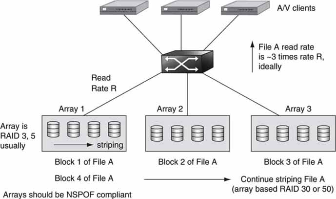
Is array striping really needed? For general-purpose enterprise data, probably not. However, if all clients need access to the same file (news footage of a hot story), then the need for simultaneous access is paramount. Take the case in which one array supports 400 Mbps of I/O, and the files are stored as 50 Mbps MPEG. If 15 clients need simultaneous dual-stream access, then the required throughput would be 15 × 2 × 50 Mbps = 1,500 Mbps. If we want to get this data throughput, the hot file should ideally be striped across at least four different arrays, providing 1,600 Mbps of read bandwidth. Many A/V systems vendors support array clustering to meet this requirement.

As it turns out, it is often easier to guarantee full availability to all files than to manage a few hot files. However, some storage vendors allow users to define the stripe width on a per-file basis. Of course, there are practical issues, such as upgrading for more storage and managing the wide stripes, but these issues can be resolved.

Striping across arrays is a multi-RAID schema. As discussed previously, RAID levels 30 and 50 are methods primarily for intra-array data and parity layout. These RAID level names can be extended to include interarray striping as well (Figure 5.13). There is no official sanction for these names, but striping across RAID sets whether intra- or inter-based is commonly done for A/V applications.

In practice, as files are striped across M arrays (a cluster), the aggregate access rates do not increase perfectly linearly. This was the case for files striped across individual HDD devices, as shown in Chapter 3A. It was reasoned that striping files across N individual disks increases the access rates but not exactly proportional to N. Also, if files are striped across M arrays, the aggregate access rate is not exactly M times the access rate of one array. Access strategies vary, and it is possible to approach a linear rate increase using clever queuing tactics (at the cost of increased R/W latency), but a deeper discussion is beyond the scope of this book.

5.2.3.1 Scaling Storage Clusters

A cluster of arrays with striped files is difficult to scale. Imagine that the storage capacity of Figure 5.13 is increased by one array, from three to four. If all files are again striped across all arrays, then each file must be restriped across four arrays. Next, the old three-stripe file is deleted. This process must be automated and can take many hours to do, depending on the array size and available bandwidth to do the restriping.

If the arrays are in constant use, then the restriping process can be very involved. Files in use (R/W) cannot be moved easily until they are closed. Files in read-only usage may be moved, but with strict care of when to reassign the file to the new four-stripe location. If the cluster is put offline for a time, then the upgrade process will be much faster and simpler. There are other strategies to scale and restripe, but this example is typical. Note that the wider the stripe (more arrays), the more risk there is of losing file data in the event of any array failure.

A few A/V vendors offer live scaling and restriping on array clusters for selected products. It is always good to inquire about scalability issues when contemplating such a system. A few of the questions to ask a providing vendor are as follows:

There are other methods of adding storage and bandwidth, but they tend to be less efficient. One method is to add mirrored storage. For read-only files (Web servers, some video servers), this works well, but for file data that are often modified, synchronizing across several mirrored copies is very difficult and can easily lead to out-of-sync data. More on mirrored storage later.

5.3 ARCHITECTURAL CONCEPTS FOR HA

“Oh, it looks like a nail-biting finish for our game. During the timeout, let’s break for a commercial.” Is this the time for the ad playback server or automation controller to fail? What are the strategies to guarantee program continuity? Of course, there are many aspects to reliable operations, but equipment operational integrity ranks near the top of the list. Author Max Beerbohm said, “There is much to be said for failure. It is more interesting than success.” What is interesting about failure? How to avoid it!

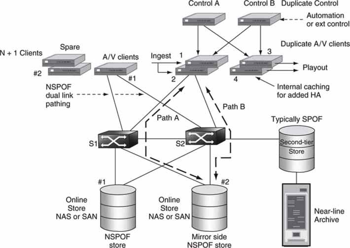
Figure 5.14 illustrates several HA methods in one system. The design exemplifies SPOF, NSPOF, N + 1 sparing, network self-healing, mirroring, and client caching. A practical design may use one or some mix of these methods. Let us examine each of them. Keep this in mind: reliability and budget go hand in hand. The more reliable the overall system, the more costly it is under normal circumstances. Paths of traditional A/V flows are not shown to simplify the diagram, but redundancy is the stock in trade to guarantee reliable operations.

FIGURE 5.14 High availability using NSPOF, N + 1, mirroring, and caching.

5.3.1 Single Point of Failure

Why use SPOF when NSPOF is available? The answer is cost and simplicity. The cost of a NSPOF robotic archive, for example, is prohibitive for most operations. The need for reliable storage decreases as the device becomes more distant from online activities. In the case of archived A/V content, most often the need for materials is predicted days in advance. Near-line storage and servers may be SPOF for similar reasons. If business conditions allow for some downtime on occasion (consistent with the availability, MTBF, and MTTR numbers), then by all means use SPOF equipment.

5.3.2 No Single Point of Failure

NSPOF designs come in two flavors: standalone devices and systems. A standalone device needs duplicated internal elements (controllers, drives, power supplies, and so on). These can be very expensive and are rare. One notable example is the NonStop brand of mainframe from HP (invented by Tandem Computers in 1975). Also, some IP switchers/routers make the claim of NSPOF compliancy. However, a system-centric NSPOF design relies on judicious SPOF element duplication to guarantee continuous operations.

It is not practical to design every system element to provide NSPOF operation. However, dual SPOF elements may be configured to act like a single NSPOF element. Critical path elements may be NSPOF in design. In Figure 5.14 there are several functionally equivalent NSPOF elements: the central switches are duplicated, some paths occur in pairs, control A and B elements are duplicated, and the ingest and playout A/V clients are duplicated. Here are a few of the ways that dual elements may be used to implement NSPOF:

In some designs, A/V clients are responsible for implementing NSPOF failover functionality. Take the case of recording ingest port #1. Path A is taken to record to online storage #2. If switch S1 faults, a connecting link faults or the online controller faults, then the client must abort the transaction and reinitiate using alternate path B. If path switching is done quickly (within buffering limits), then none of the input signal will be lost during the record process.

For bulletproof recording, an ingest client may record both to online stores #1 and #2 using a dual write scheme. This keeps the two stores in complete sync and guarantees that even if one fails, the other has the goods. Additionally, an input signal may be ingested into ports #1 and #2 for a dual record. Either port may fail, but at least one will record the incoming signal.

Because NSPOF designs are costly, is there a midstep between SPOF and NSPOF? Yes, and it is called N + 1 sparing.

5.3.3 N + 1 Sparing

While NSPOF designs normally require at least some 2 × duplication of components at various stages, N + 1 sparing requires only one extra, hot spare, out of N elements. It is obvious that this cuts down on capital cost, space, and overall complexity. So how does it work?

Let us consider an example. Say that N Web servers are actively serving a population of clients. An extra server (the + 1) is in hot standby, offline. If server #K fails, the hot spare may be switched into action to replace the bad unit. The faulty unit is taken offline to be repaired. Of course, the detection of failure and subsequent switching to a new standby unit require some engineering. Another application relates to a cluster of NAS servers. In this case, if a server fails out of a population, it must be removed from service, and all R/W requests are directed to a hot standby. For example, if the clients accessing the NAS are A/V edit stations (NLEs), then they must have the necessary logic to monitor NAS response times and switch to the spare. Each client has access to a list of alternate servers to use in failover. Failover is rarely as smooth as with NSPOF designs, as there will be some downtime between fault detection and rerouting/switching to the spare. Also, any current transaction will likely be aborted and restarted on the spare. Most NLEs do not support client-based storage failover, but the principle may be applied to any A/V client.

Of course, N + 2 sparing (or N + K in general) is better yet. The number of spares is dependent on the likelihood of an element failure and business needs. Some designs select “cheap” elements knowing that N + K sparing is available in the event of failure. This idea is not as daffy as it first sounds. In fact, some designs shun NSPOF in favor of N + K to cut equipment costs, as NSPOF designs can become costly. This is a good trade-off based on the trends shown in Figure 5.1.

Let us consider one more example. In Figure 5.15 there are N active video server I/O devices under control of automation for recording and playback. If device #2 fails, then by some means (automatic or manual) the recording and playout may be shifted to the spare unit.

FIGURE 5.15 N + 1 sparing for a bank of video server nodes.

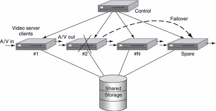
Of course, this also requires coordination of input and output signal routing. Also, this works best when all stored files are available to all clients. In some practical applications, N + 1 failover occurs with a tolerable delay in detection and rerouting. We must mention that not all automation vendors support N + 1 failover. However, all automation vendors do support using the brute-force method or running a complete mirror system in parallel, but this requires 2 N clients, not N + 1. Another vital aspect of AV/IT systems is network reliability. A failure of the network can take down all processes. HA networking is discussed next.

5.3.4 Networking with High Availability

Let us dig a little deeper into the methods for creating a high-availability networking infrastructure. Figure 5.16 illustrates a data routing network with alternate pathing and alternate switching. The concepts of layer 2 and layer 3 switching, routing protocols, and their failover characteristics are discussed in Chapter 6.

FIGURE 5.16 Data routing with alternate pathing and switching.

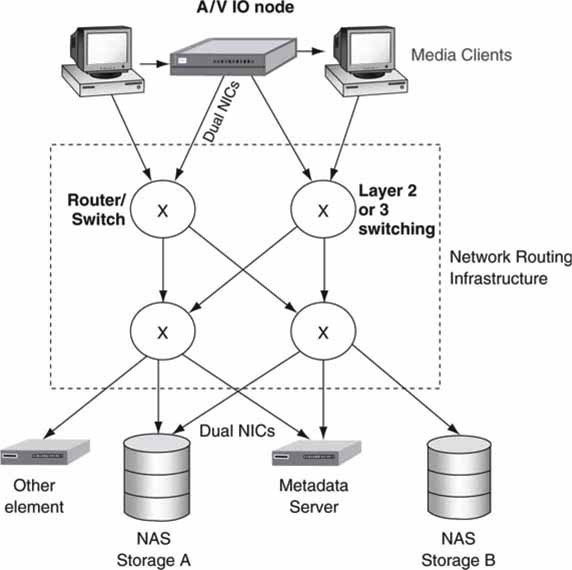
Figure 5.16 has some similarities to Figure 5.14. In addition to client-side route/path control, it is possible to create a network that has self-healing properties. It is always preferred for the network to transparently hide its failures than to invoke the client to deal with a network problem. For example, if one switch fails, packets may be routed over a different path/switch as needed. There are various routing and switching protocols, and each has its own specific automatic failover characteristics. Frankly, layer 2 switching is very practical for A/V workflow applications using small networks. Layer 3 is more advanced in general but can be used to route real-time A/V for more complex (including geographically separated) workflows.

Keep in mind that networked systems may introduce occasional delays that are not necessarily hard faults. For example, a local DNS cache may time out, requiring a delay in resolving a name to a numerical IP address. Routing tables too may need updating, causing a temporary and infrequent delay. These delays may occur at the most inopportune moment, so you need to plan for them or design them out.

Finally, there is a method (not shown) for creating a fault-tolerant “virtual router” using a pair of routers. One router is in standby, while the other is active. The Virtual Router Redundancy Protocol (VRRP, RFC 2338) performs an automatic failover between the two routers in the event that the active one fails. All connecting links attach to both routers, so there is always routed connectivity via one switch or the other. In effect, VRRP creates a NSPOF-configured router.

5.3.5 Mirroring Methods

In 1997 Alan Coleman and his geneticists amazed the world when his team cloned a sheep. Dolly became a household name. Cloning sheep holds little promise for A/V applications, but cloning data—now that is a different story. Cloned data are also called a data mirror. So how can mirroring juice up storage reliability?

If used in conjunction with N + 1 and NSPOF methods, mirrors provide the belt-and-suspenders approach to systems design. Mirrors may include the following:

One of the main worries when using a storage mirror is keeping them 100 percent identical. If one side of mirrored storage fails, then the other unit will likely contain new files by the time the storage is repaired. If this happens, some resync operation needs to occur to guarantee true mirrored files. This should be automatic. Using mirrors is usually based on business needs. If they can be avoided, the overall system is simplified.

5.3.6 Replication of Storage

Storage replication is a poor man’s mirror. Replicated storage is a snapshot in time of the primary source. As the primary storage is modified, the secondary one is updated as fast as business needs allow for. If the secondary storage is connected via a low bandwidth WAN, then the syncing may lag considerably. For read-centric applications where the primary storage changes infrequently, replication is a better bet than a sophisticated mirror approach. The secondary storage may be of lesser performance and, hence, less costly. If the primary storage fails, then some logic needs to kick in to use the secondary files. Many A/V system vendors and integrators can provide storage replication functionality.

Storage backup (tape, optical) finds a place in A/V systems too. Inexpensive backup will have slow recovery times, so design accordingly. Backup is the not the same as archive. Archive content lifetime may be 50 years, whereas most backups last days or weeks. Some A/V systems keep a spare copy only as long as the near-line or online store has the working copy. As a result, the save time can vary depending on schedules and use patterns.

5.3.7 Client Caching Buys Time

Client local caching (~buffering) also provides a measure of HA. Figure 5.14 shows several clients with A/V outputs. The main programming source files for playout come from either online or near-line storage. Usually, each playout client also has a measure of local storage. If the programming is known in advance (e.g., broadcast TV), then the local client cache may be prefilled (prequeued) with target files. When playout starts, files are read from local memory and not directly from any external stores. With sufficient buffering, it is possible to cut the umbilical cord between the playout (or ingesting) client and external storage with no ill effects for some set time. In fact, a client may play out (or record) hours’ or days’ worth of A/V even though the main storage and connecting infrastructure are down. If the playout or record schedule is also cached in the client, then all client operations are independent of external control or storage. For sure, local caching increases the overall system reliability. Refer to Figure 3B.22 and associated text for more insights into the advantages of caching.

Many control schemas do not support local caching, preferring to run directly from online storage. One issue is last-minute changes. Given a list of prequeued files, they may need to be flushed if the schedule changes at the last minute. This may happen in a live news or sports program. The control logic is more complex with caching but worth the effort to gain the added reliability. Also, running off local client-based storage relaxes the QoS of the external storage and connecting infrastructure, as the queuing step may be done in NRT under most circumstances. Also, the internal storage will need to support the required bandwidth (say for HD rates), not just the needed storage capacity. As A/V vendors make their products more IT friendly, expect to see more use of client caching.

One more use of local client caching is for remote operations. If the A/V client is remote from the main storage, providing a reliable WAN-based QoS can be costly. With proper client caching, remote clients may offer a high level of reliability, despite a low-grade link to main storage. This technique works best when the record/playout schedules are stable and known in advance. Remote clients are sometimes called edge clients because they are at the edge of a network or system boundary.

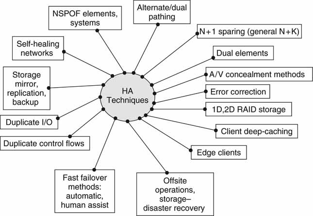
Figure 5.17 summarizes the main themes discussed so far. It is a good reminder of the choices that systems designers have at their disposal when configuring HA systems. There are other methods to build HA systems and the next section focuses on some novel approaches.

FIGURE 5.17 Summary of high-availability techniques.

5.3.8 Other Topologies for HA

Currently, there is industry buzz about the virtual data center, virtual computing, and utility computing. Each of these describes a variant of a configuration where requests for services are routed to an available resource. Imagine a cluster of servers, clients, processors, and networks all offered as undedicated resources. A managing entity can assign “jobs” to server/client/network resources; when the job is complete, the resource is released and returned to the pool, ready for the next assignment. If one resource faults, another can take its place, although not always glitch-free in the A/V sense.

In enterprise IT, these new paradigms are capturing some mind share. The sense of a dedicated device statically assigned a fixed task is replaced by a pool of resources dynamically scheduled to perform as needed. Reliability, scalability, and flexibility are paramount in this concept. This idea has not yet been embraced by A/V systems designers, but the time will come when virtual computing will find some acceptance for select A/V (encoding, decoding, format conversing, conforming, etc.), control (scheduling, routing), and storage (NAS servers) processes. Although not yet applicable to A/V applications (other than searching methods), one particularly interesting no-fault design is that used by Google (Barroso). It has configured ~500,000 “unreliable” SPOF servers linked to form huge searching farms located worldwide. Query terms (video + IT + networking) are split into “shards,” and each shard is sent to an available search engine from a pool of thousands. The results of each shard query are intersected, and the target sites are returned to the client. The system scales beautifully and can withstand countless server failures with little impact on overall performance. There has been speculation that a Google-like architecture may be offered as a utility computing resource, ready for hire. This is an exciting area, ripe for innovation.

5.3.9 Concealment Methods

When all else fails, hide your mistakes. Sound familiar? Not only does this happen with human endeavors, A/V equipment does it as well. It is not a new idea; when a professional VTR has tape dropout problems, the output circuitry freezes the last good frame and mutes the audio until the signal returns. Concealing problems is preferred to viewing black or jerky video frames or hearing screeching audio. Similar techniques may be used when a device receives corrupted data over a link or data are late in arriving from storage. A good strategy is to hold the last good video frame and to output the audio if it has integrity or else mute it. When you are recording an A/V signal that becomes momentarily corrupt, it is good practice to record the last valid frame along with any good audio until signal integrity returns. It is preferable to conceal problems than to fault, display, or record garbage.

5.3.10 A Few Caveats

When specifying an HA design, always investigate what the performance is after a failure. Is it less than under normal operations, is the failover transparent, and who controls the failover—man or machine? Also, what is the repair strategy when an element fails? Can the offending element be pulled without any reconfiguring steps? When a faulty element is replaced, will it automatically be recognized as a healthy member of the system? What type of element reporting is there? HA is complex, so ask plenty of questions when evaluating such a design.

5.4 SCALING AND UPGRADING SYSTEM COMPONENTS

So, the system is working okay and everyone is happy. Then upper management decides to double the number of channels or production throughput or storage or whatever. The first question is, “Can our existing system be scaled to do the job?” The wise systems designer plans for days like this. What are some of the factors that are important in scaling AV/IT systems? Here is a list of the most common scale variables:

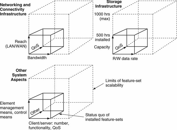
Figure 5.18 illustrates each of the scale dimensions as legs of a cube.² The smaller volume cubes represent the current or status quo feature sets. The larger volume cubes represent the top limits of the same feature sets. Assume, for example, that the current storage capacity is 500 hr of A/V files but that the maximum practical, vendor-supported size is 1,000 hr. These values are indicated on the storage cubes in Figure 5.18. Generally, exceeding the maximum rate requires an expensive forklift upgrade of some kind. Knowing the maximum dimensions of each large cube sets limits on the realistic, ultimate system scalability. Incidentally, not every possible scale parameter is specifically cited in Figure 5.18. Hence, make sure you identify the key factors that are of value to you when planning overall system scalability.

FIGURE 5.18 Key dimensions of system scalability.

When selecting a system, always seek to understand how each of the dimensions should be scaled. Of course, guaranteeing a future option to scale in one area or another will often cost more up front. If 5TB of storage capacity is sufficient at system inauguration, how much more will it cost for the option to expand to 20TB in the future? This cost does not count the actual expansion of 15TB, only the rights to do it later. Paying for potential now may pay off down the road if the option is exercised. Sometimes it is worth the cost; sometimes it is not.

It is likely though, at some future time, that some change will be asked for, and the best way to guarantee success is to plan for it to a reasonable degree. When the boss says “Boy, are we lucky that our system is scalable,” you can think, “It is not really luck, it is good design.” Yes, luck is a residue of good design.

5.4.1 Upgrading Components

Independent of scaling issues, all systems will need to be upgraded at some point. At the very least, some software security patch will be required, or else you may live in fear of a catastrophe down the road. Then there are performance upgrades, HW improvements, bug fixes, mandatory upgrades, OS service patches, and so on. If system downtime can be tolerated during part of a day or week, then upgrades are not a big deal. However, what if the system needs to run 24/7? Well, then the upgrade process depends on how the clients, infrastructure, and storage are configured and their level of reliability.

If the principles of NSPOF, N + 1, replication, and mirroring are characteristics of the system design, then “hot” upgrades (no system downtime, performance not degraded) are possible. It is easy to imagine taking the mirror side out of service temporarily to do an upgrade, removing a client from operation knowing that the spare (N + 1) can do the job, or disabling an element while its dual (NSPOF) keeps the business running. In some cases, an element may be upgraded without any downtime. Increasing storage capacity may be done hot for some system designs, whereas others require some downtime to perform the surgery.

Always ask about hot upgrade ability before deciding on a particular system design. In a way, the ability to upgrade is more important than the option to scale. The reason is that upgrades will happen with 100 percent certainty except to the most trivial elements. However, future system scaling may never happen.

5.5 IT’S A WRAP—SOME FINAL WORDS

Yes, sometimes things do not always go from bad to worse, but you cannot count on it. Anyone who has been hit hard by Murphy’s Law will know the only way to outwit Mr. Murphy is to hire him as a consultant. Andy Grove of Intel famously said, “Only the paranoid survive.” When it comes to reliable operations, it is okay to be paranoid. Planning for the worst-case scenario is healthy thinking, especially if it leads to worry-free sleep and a system that just keeps humming along.

REFERENCES

Barroso, L. A., et al. (March 2003). Web Searching for a Planet: The Google Cluster Architecture. IEEE Micro Magazine, 23 (2), 22–28.

The Mythical Man-Month: Essays on Software Engineering, Fred Brooks, Addison-Wesley Professional; 2nd edition (August 12, 1995).

Proceedings of the 1988 ACM SIGMOD International Conference on Management of Data, Chicago, Illinois, United States Pages: 109–116. Year of Publication: 1988. ISBN: 0-89791-268-3.