CHAPTER 6
Networking Basics for A/V
CONTENTS
6.1.1 Physical and Link Layers
6.1.3 The Transport Layer —TCP and UDP
6.3.1 Screaming Fast TCP/IP Methods
6.3.2 TCP Offl oad Engines (TOEs)
6.3.3 A Clever Shortcut to TCP Acceleration
6.4 The Wide Area Network (WAN)
6.4.1 WAN Connectivity Topologies
6.5 Carrier Ethernet (E-LAN and E-Line)
6.6 Understanding Quality of Service for Networks
6.6.2 QoS Classifi cation Techniques
6.6.3 QoS Reservation Techniques
6.7 It’s a Wrap—Some Final Words
6.0 INTRODUCTION
The kingpin of all of IT communication technologies is the network. Fortunately, we live at a time when there is one predominant network, and it is based on the Internet Protocol (IP). Gone are the days when IP and AppleTalk and IBM’s SNA and Novell’s IPX all competed for the same air. Gone are the days when clumsy protocol translators were required to move a file between two sites. Yes, gone are the days of network chaos and incompatibility. Welcome IP and its associated protocols as the world standard of communications networks. Without IP, there would be no Internet as we know it.
This chapter just touches on the basics of networking principles. The field is huge, and there are countless books and Web references (see www.ietf.org and www.isoc.org) dedicated to every nook and cranny of IP networking. See also (Stallings 2003) and (Stevens 1994) for information on IP and associated Internet protocols. The focus combines an overview of standard networking practices with special attention to A/V-specific needs, such as real-time data, live streaming over LAN and WAN, high bandwidth, and mission-critical QoS metrics. It is the intersection of A/V and networking that is most interesting to us. Let us begin with the classic seven-layer stack.
6.1 THE SEVEN-LAYER STACK
No discussion of networking is complete without the seven-layer stack. Figure 6.1 shows the different layers needed to create a complete end-to-end networking environment. The original Open Systems Interconnection (OSI) model is used as a reference by which to compare the Internet and other protocol stacks. The OSI stack itself may be split into three coarse levels: link access layer, transport layer, and applications layer.
FIGURE 6.1 The OSI model and Internet stack.
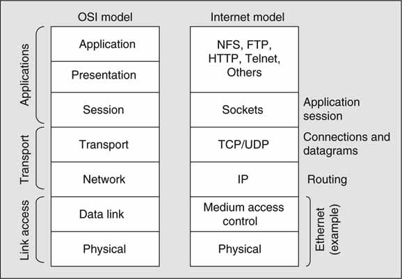
The lowest level of the three coarse layers is the physical and link access (addressing, access methods) layer. The transport layer relates to moving data from one point in the network to another. The application layer is self-evident. The Internet stack does not have an exact 1:1 correspondence to every OSI layer, but there is no requirement for an alignment. Each layer is isolated from the others in a given stack. This is good and allows for implementations to be created on a per-layer basis without concern for the other strata.
Figure 6.2 shows the value of isolated layers. There is a peer-to-peer relationship between each layer on the corresponding stacks. A layer 2 switch (e.g., Ethernet I/O) operates with knowledge of the physical and data link levels only. It has no knowledge of any IP or transport layer activity. Another example is the IP router (or IP switch). It follows the rules of the Internet Protocol for switching packets but is unaware of the levels above or below. At the transport level, a TCP accelerator (HW-based TCP processor) can function without knowledge of the other layers as well.
FIGURE 6.2 Layer processing using peer-to-peer relationships.
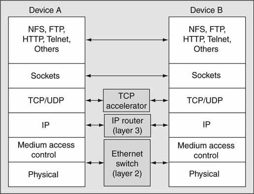
Of course, some devices may need to comprehend several layers at once, such as a security firewall (or intrusion prevention device) that peeks into and filters data packets at all levels. However, each layer-process may still operate in isolation. The genius of peer-to-peer relationships has enabled stack processors to be designed and implemented independently with a resulting benefit to testing, integration, and overall simplicity.
![]() One quick way to remember the order and names of the layers is the acronym PLANTS. From the bottom up it is P (physical), L (link), A (okay, just say and), N (network), T (transport), and S (session). Of course, the presentation/application layers are always at the top.
One quick way to remember the order and names of the layers is the acronym PLANTS. From the bottom up it is P (physical), L (link), A (okay, just say and), N (network), T (transport), and S (session). Of course, the presentation/application layers are always at the top.
Let us examine the layers in more detail. At the top of the stack are applications such as FTP, NFS, Web access via HTTP, time-of-day, and so on. The most common applications are available on desktops and servers as standard installs. For a list of all registered applications using well-known ports, see www.iana.org/assignments/port-numbers.
Immediately below the presentation/application layers is the session layer. A session is established between a local program and a remote program using sockets. Each end point program uses a socket transaction to connect to the network. Program data are transferred between end point programs using TCP/IP or UDP/IP. Sockets have their own protocol for setting up and managing the session. From here on, let us study the stack from the bottom up, starting with the physical and link layers.
6.1.1 Physical and Link Layers
Ethernet is the most common representation of the bottom two layers for local area network (LAN) environments and has won the war of connectivity in the enterprise IT space. Just a few years ago, it battled against Token Ring and other LAN contenders, but they were knocked out. In addition to LANs, WANs, MANs, satellite links, DSL, and cable modem service provide link layer functionality. WANs and MANs are considered later in this chapter.
One that has become a favorite in the Telco arena is called Packet Over SONET (POS). With POS, IP packets are carried over a SONET link. Another useful IP carrier is an MPEG Transport Stream as deployed in satellite and cable TV networks. Terrestrial transmissions using ATSC, DVB, and other standards also carry IP within the MPEG structure. The common DSL modem packages TCP/IP for carriage over phone lines. Ethernet too has been extended beyond the enterprise walls under the new name Transparent LAN (TLAN). This is a metropolitan area network (MAN) that is Ethernet based. TLANs and SONET are discussed in the WAN/MAN section later in this chapter. For now, let us concentrate on Ethernet as used in the enterprise LAN.
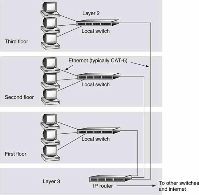
Ethernet was invented in 1973 by Robert Metcalfe of Xerox. It was designed as a serial, bidirectional, shared media system where many nodes (PCs, servers, others) connect to one cable. Sharing a snaked cable among several devices has merit, for sure. Unfortunately, because any one node can hog all the bandwidth, shared media have given way to central switching (star topology). This has become de rigueur for LANs, and each node has a direct line to a switch or hub. Figure 6.3 shows a typical star configuration of Ethernet-connected nodes. The star is ideal for A/V networking, as it offers the best possible QoS, assuming that congestion (packet loss) in the switches is low or nonexistent.
FIGURE 6.3 Hierarchical switching example.
Ethernet specs are controlled by the IEEE, and 802.3X is a series of standards for defining the range of links from 10 Mbps to the top of the line 10 Gbps. There are 12+ defined wire/fiber specifications. The most common spec is CAT-5 wiring, which supports 100Base-TX (100 Mbps line rate) and 1000Base-T Ethernet. CAT-5 cable is four twisted and unshielded copper pairs. 100Base-TX uses two pairs, and 1000Base-T uses four pairs.
Ten Gbps rates demand fiber connections for the most part, although there is an implementation using twin-axial cable instead of the more common Category 5 cabling. 10G line coding borrows from Fibre Channel’s 8 B/10 B scheme (see Appendix E) as do the first three links in the following list. Common IEEE-defined gigabit Ethernet links are
• 1000Base-LX from 500M (multimode fiber) to 5km (single mode fiber)
• 1000Base-SX from 220M to 550M (multimode fiber)
• 1000Base-CX at 25M copper (82 feet)
• 1000Base-T, copper Cat 5, 100M (327 feet) (five-level modulation)
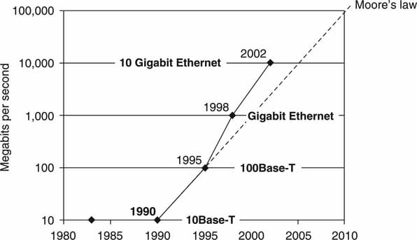
10G links will not connect to PCs but rather as backbone transport between IP switchers and routers and some servers. There is no reason to stop at 10G rates. The IEEE is standardizing 40 and 100 Gbps rates using both fiber and 10 meter copper. Figure 6.4 gives a history of Ethernet progress. Note that the current development run rate is beating Moore’s law.
FIGURE 6.4 The evolution of Ethernet.
6.1.1.1 Ethernet Frames
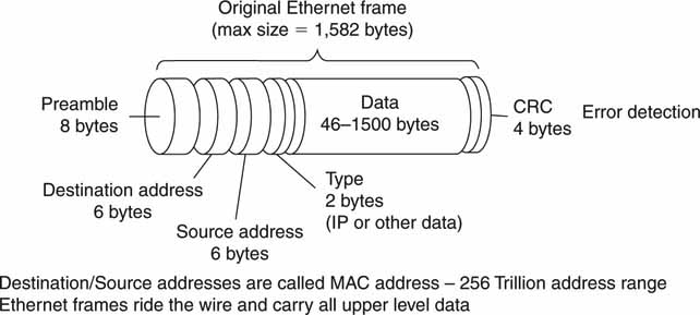
The on-the-wire format to carry bits is the Ethernet frame, as shown in Figure 6.5. As with most packet protocols, there is a preamble and address field followed by the data payload (1,500 bytes max, nominal) field concluded by an error detection field. So-called jumbo frames carry payloads of sizes >1,500 up to 9,000 bytes. Jumbo frames are processed more efficiently with less framehandling overhead. Each Ethernet port has a worldwide 48-bit Medium Access Control (MAC) address that is unique per port. MAC addressing supports 256 trillion distinct ports. MAC addressing is used for many link types—not just Ethernet. Do not confuse this address with an IP address, which is discussed in the next section. Some network switches use the MAC address to forward frames. This mode of frame routing is often called layer 2 switching. Layer 2 switching is very limited in its reach compared to IP routing, as we will see.
FIGURE 6.5 The Ethernet frame.
Ethernet frames are sent asynchronously over the wire/link. There is no clock for synchronous switching as there is with a SDI signal. So any real-time streaming of A/V data must account for this. Several commercial attempts have tried to turn Ethernet into a time-synchronous TDMA medium, but they have not succeeded, despite the obvious advantages for A/V transport. See Chapter 2 for more information on using asynchronous links to stream synchronous A/V.
Let us move one layer higher in the stack to the network layer. This layer’s entire data field is carried by the Ethernet frame.
6.1.2 The IP Network Layer
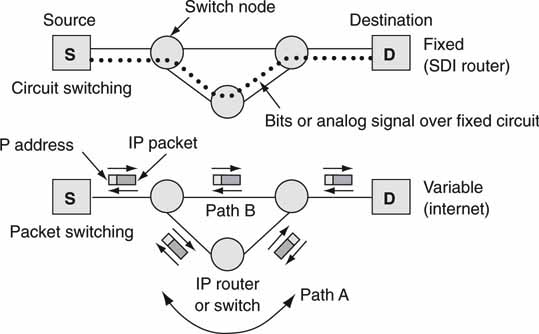
The IP network layer is the IP routing layer. There are many ways to route signals (data) from source to destination. One way is called circuit switching, which is typified by the legacy telephone system. In this case, a telephone call is routed via switches to form a literal circuit from source to destination. The circuit stays intact for the duration of the call, and the QoS of the connection is excellent. The traditional SDI router is circuit switched (crossbar normally) and connects input ports to output ports with outstanding QoS. Circuits must be set up by some external control.
On the other hand is packet switching. As an example of packet routing, let us use the analogy of sending a picture postcard of the Chelsea Bridge from London to 385 Corbett Avenue, San Francisco, USA. The postcard (a packet) enters the post office system and is routed via various offices until it reaches its destination. A clerk, or machine, at a London post office examines the destination address and forwards the packet to Los Angeles, USA. Next, the LA post office forwards the packet to the main post office in San Francisco with subsequent forwarding to the local post office nearest Corbett Avenue. At each step the destination address is examined, and the packet is forwarded closer to the final address.
In the end, a letter carrier hand delivers the postcard packet to street address 385. If the destination address cannot be located, then a return message is sent (“return to sender”). It is not uncommon to simultaneously mail two postcards to the same address and have them arrive on different days. One card may traverse via New York City while another traverses via LA, so although the routes are different, the final destination is the same. Welcome to the world of packet routing. This type of routing is often called layer 3 routing. Figure 6.6 shows examples of circuit and packet-switched methods. Layer 2, MAC switching, is similar to layer 3, but there are differences, as will be shown.
FIGURE 6.6 Example of circuit and packet routing.
As with the Ethernet frame, each packet has an address field (the IP address) and payload field. Some of the features of a packet routing are as follows:
• Because each packet has a destination (and source) address field inspected at each routing point, packets are self-addressing—not true with circuit switching.
• Policies (routing protocols) decide how to route each packet—via LA or NYC?
• Congestion may cause some packets to be delayed or even dropped—the Christmas card syndrome.
• Packets are not error corrected (at higher stack levels they are, however).
• Packets associated with the same stream may take different routes (hops), resulting in out-of-order packet reception at the receiver (path A or B in Figure 6.6).
• Packets may exhibit jitter (variation in delay) during the life of the stream.
• The QoS is difficult to guarantee in large networks.
• Packets are carried by the lower two layers in the stack (e.g., Ethernet frames).
As a result, packet switching lacks some of the more A/V-friendly features of circuit switching. Despite this, packet switching offers self-addressing, resiliency to router failure, wide area routing, and IT-managed and relatively inexpensive switches. The best success story for packet switching is the Internet. Imagine building the Internet from circuit-switched elements. Some entity would need to open/close every switch point, and this alone signals disaster for such a topology.
The biggest issue of using packets (compared to circuit switching) to move A/V data is a potentially low or unspecified QoS. As discussed in Chapter 2, there are clever ways to smooth out any packet jitter; using TCP (next layer in the stack), any packet errors may be 100 percent corrected. So the only real issue is overall latency, which may be hidden or managed in most real-world systems.
Over small department networks, the latency through several switch hops may be well controlled. It is possible to achieve a <30-μs end-to-end latency for such a network. This is less than one raster line of video in length. As a result, real-time streaming and device control using routed packets is practical. Of course, a 30-μs end-to-end delay is not common for most networks, but the principle of low-latency networks is well established.
6.1.2.1 Comparing Layer 2 and Layer 3 Switching
This section sorts out some of the pros and cons of layer 2 and layer 3 switching. In many enterprise networks, switches route Ethernet frames using the MAC address (layer 2 switching) or packets using the IP address (layer 3 switching). Many commercial switches support both methods. See Figure 6.3 for a simple network using both layer 2 and 3 switching. Medium to large network domains use a mix of layers 2 and 3, whereas smaller networks or LAN subgroups use only layer 2 methods. There are trade-offs galore between these two methods, but the main aspects are as follows:
1. Layer 2 switching domain
• Switching is based on MAC address in Ethernet frame.
• It supports small/medium LAN groups or VLANs that confine broadcast messages but provides limited scalability.
• It offers excellent per-port bandwidth control.
• Path load balancing is not supported.
• Spanning Tree Protocol (STP) supports path redundancy while preventing undesirable loops in a network that are created by multiple active paths between nodes. Alternate paths are sought only after the active one fails.
• It is easy to configure and uses lower cost switches than layer 3.
2. Layer 3 switching (routing) domain
• Switching is based on the IP address.
• It scales to large networks—departments, campus networks, the Internet.
• It routes IP packets between layer 2 domains.
• Redundant pathing and load balancing are supported.
• It is able to choose the “least-cost” path to next switch hop using Open Shortest Path First (OSPF) or older Routing Information Protocol (RIP) routing protocols. OSPF has faster failover (<1 s possible) than STP.
Layer 2 and 3 switching can live together in complete harmony. It is quite common for portions of a network design to be based on layer 2 switching while other portions are based on layer 3. For A/V designs, layer 2 can offer excellent QoS at the cost of slow failover if a link or node fails. STP can take 30–45 s to find a new path after a failure is detected. For this reason, RSTP is sometimes used. Rapid STP, based on IEEE standard 802.1 W for ultrafast convergence, is ideal for A/V networks. See (Spohn 2002) for a good summary of layer 2 and 3 concepts and trade-offs. See also (DiMarzio 2002) for a quick summary of routing protocols of concepts or scour the Web for information.
Another aspect of layer 2 is deterministic frame forwarding. In most cases, Ethernet frames will traverse links according to the forwarding tables (built using STP) stored in each switch. The packet forwarding paths are static,1 until a link or switch fails. Then, if possible, a new path will be discovered by STP, and packet forwarding continues. In a static network, for example, media clients accessing NAS storage should see a fixed end-to-end delay plus any switchinduced jitter for each Ethernet frame.
However, layer 3 can route over different paths to reach the same end point. Because routing occurs on a per-packet basis, this will likely introduce added jitter above what layer 2 switching introduces. See Figure 6.6 for an example of alternate pathing (path A or path B may be used as determined by routing protocols) using layer 3 routing. See Chapter 5 on how to build fault-tolerant IP routing networks. In the end, judicious network design is needed to guarantee a desired QoS and associated reliability.
![]() The primary difference between a layer 3 switch and a router depends more on usage than features. Layer 3 switching is used effectively to segment a LAN rather than connect to a WAN. When segmenting a campus network, for instance, use a router rather than a switch. When implementing layer 3 switching and routing, remember: Route once, switch many.
The primary difference between a layer 3 switch and a router depends more on usage than features. Layer 3 switching is used effectively to segment a LAN rather than connect to a WAN. When segmenting a campus network, for instance, use a router rather than a switch. When implementing layer 3 switching and routing, remember: Route once, switch many.
6.1.2.2 IP Addressing
Just as a house has a street address, networked devices have IP addresses. The IP (IPV4) address is a 4-byte value. The address range is split into three main classes: A, B, and C. Each class has a subdivision of network ID and host ID. What does this mean? A network ID is assigned to a company or organization depending on the number of host IDs (nodes on their network) (see Figure 6.7). Classes A, B, and C are for point-to-point addressing. A special class D address is reserved for point-to-multipoint data transfer.
FIGURE 6.7 IP addressing concepts.
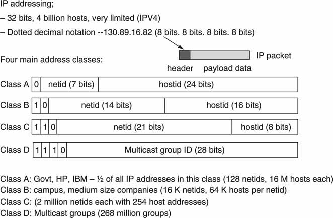
For example, MIT has a class A network ID (netid) of 18, and the campus can directly support 16 million hosts (2^24). A smaller organization may be assigned a class C address that supports only 256 hosts. Many addresses have an equivalent network name as well. For example, MIT’s IP Web address is http://18.7.22.83 (in so-called dotted decimal notation) and its equivalent name is http://www.mit.edu. A network service called a Domain Name Server (DNS) is available to look up an address based on a name. Numeric addresses, not names, are needed to route IP packets.
To better understand IP addressing, DNS address lookup, ping (addressed device response test), trace route (a list of hops), and other network-related concepts, visit www.dnsstuff.com for a variety of easy-to-run tests. Ten minutes experimenting with these tests is worth the effort. Note that it takes time (<100 Ms usually) to look up an IP address based on a name. In time-critical A/V applications, it is often wise to use numeric addresses and avoid the DNS lookup delay. As a result, http://www.mit.edu takes slightly longer to reach than http://18.7.22.83 if the named address is not already cached for immediate use.
6.1.2.3 Subnets
A class A address space supports 16 million hosts. All the hosts on the same physical network share the same broadcast traffic; they are in the same broadcast domain. It is not practical to have 16 million nodes in the same broadcast domain. Imagine 16 million hosts broadcasting data packets! Now that is a data storm. The result is that most of the 16 million host addresses are not usable and are wasted. Even a pure class B network with 64K hosts is impractical.
As a result, the goal is to create smaller broadcast domains—to wall off the broadcast traffic—and to better utilize the bits in the host ID (hostid) by subdividing the IP address into smaller host networks. The basic idea is to break up the available IP addresses into smaller subnets. So a class B host space may be divided into say 2,048 (11 bits of host ID) subnets each with ~32 hosts (5 bits of host ID)—a very practical host size. In reality, the host ID cannot be perfectly subdivided to utilize every possible host address. Still, subnetting is a practical way to build efficient networks. Each subnet shares a common broadcast domain, and each is reachable via IP, layer 3, and switches/routers that bridge domains.
![]() Layer 2 Versus Layer 3 Switching: Layer 2 switching uses the MAC address in the Ethernet frame to forward frames to the next node. Layer 3 switching uses the IP address in the IP packet to forward packets.
Layer 2 Versus Layer 3 Switching: Layer 2 switching uses the MAC address in the Ethernet frame to forward frames to the next node. Layer 3 switching uses the IP address in the IP packet to forward packets.
6.1.2.4 IPV6 and Private IP Addresses
No doubt about it, the Internet is running out of IP addresses. The day is near when every PC, mobile phone, microwave oven, and light switch (or even light bulb) will require an IP address. There are two solutions to this problem. One is to migrate to the new and improved version of IP, IPV6 (RFC 2460). Among other valuable enhancements, each IP packet has a 128-bit address range, which is ~1038 addresses. This is equivalent to 100 undecillion2 addresses. There are an estimated 1028 atoms in the human body, so IPV6 should suffice for a while. IPV6 is slowly being adopted and will replace IPV4 over time. There are transition issues galore, as may be imagined. One transition scenario is to support dual stacks—IPV4 and IPV6—in all network equipment. This is not commonly done but may become so as IPV6 kicks into gear.
A more common solution for living with the limited IPV4 address space is to use the Network Address Translation (NAT) method. Several addresses have been set aside for private networks as listed in Table 6.1. These addresses are never routed on the open Internet but only in closed, private networks.
Table 6.1 Dedicated Private IP Address Ranges
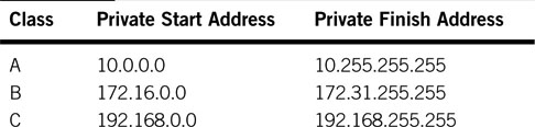
The NAT3 function is similar to what a telephone receptionist does. The main office number is published (a public IP address), but the internal phone network has its own extension numbering plan (private IP addresses) not directly accessible from the outside. The operator routes incoming calls to the correct extension by doing address and name translation. Because the private IP addresses are never routed on the open Internet, they may be reused as often as needed in private networks just as phone extension numbers are reused by other private phone systems.
NAT has effectively added billions of new virtual IP addresses, which has stalled the uptake of IPV6. Many companies use NAT services and rely on pools of internal, private IP addresses for network nodes. Many modern A/V systems (playout servers, news production systems, edit clusters) also use private IP addresses. NAT uses several methods to map internal private to external public IP addresses. To learn more, see http://computer.howstuffworks.com/nat1.htm.
The IP layer is replete with protocols to assist in routing packets over the open terrain of the Internet. For the most part, they do not influence A/V networking performance, so they are not covered. There is one exception: QoS. Network QoS is governed by several net protocols, which are reviewed later in this chapter. IP multicast is useful when streaming an IP broadcast to many end stations. The next section outlines the basics.
6.1.2.5 IP Multicasting
Multicasting is a one-to-many transmission, whereas the Internet is founded on unicast, one-to-one communications. Plus, multicasting is normally unidirectional, not bidirectional, as with, say, Web access. Multicast file transfers are not common, but there are ways to do it, as discussed in Chapter 2. See also www.tibco.com for a variety of file distribution solutions to many simultaneous receivers.
The IP class D address is reserved for multicast use only. In this case, each host ID is a multicast domain, like the channel number on a TV. Any nodes associated with the domain may receive the IP broadcast. IP multicast is a suite of protocols defined by the IETF to set up, route, and manage multicast UDP packets. Most multicast is best effort packet delivery, although it is possible to achieve 100 percent transfer reliability. This is not common and becomes complex with a large number of receivers.
The key to multicasting is a multicast-enabled routing system. Each router in the network must understand IP multicast protocols and class D addressing. IP packets are routed to other multicast-enabled routers and to end point receivers. Any node that tunes into an active class D host address will be able to receive the stream.
The Internet in general does not support IP multicasting for a variety of reasons. The protocols are complex, and there is no easy way to charge for multicast packet routing and bandwidth utilization. Imagine a sender who establishes a multicast stream to one million receivers that span 100 different Internet service providers. The business and technical challenges with this type of broadcast are intricate, so ISPs avoid offering the capability. However, campus-wide multicast networks are practical and in use for low bit rate streaming video applications. There is very little IP multicast used for professional A/V production. Next, let us focus next on the granddaddy of all protocols, TCP and its cousin UDP.
6.1.3 The Transport Layer—TCP and UDP
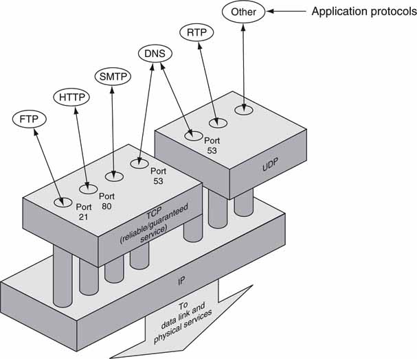
Transmission Control Protocol (TCP) is a subset of the Internet Protocol suite often abbreviated as TCP/IP. TCP sits at layer 4 in the seven-layer stack and is responsible for reliable data communications between two devices. Figure 6.8 provides a simple view of TCP’s relation to application-related protocols, UDP, and lower levels. Consistent with stack operations, TCP packets are completely carried as payload by IP packets. TCP supports full duplex, point-to-point communications.
FIGURE 6.8 TCP and UDP in relation to application protocols.
Concept: Encyclopedia of networking and telecommunications.
The TCP packet format is described in Figure 6.9. Some notable characteristics are as follows:
FIGURE 6.9 General layout of a TCP packet.
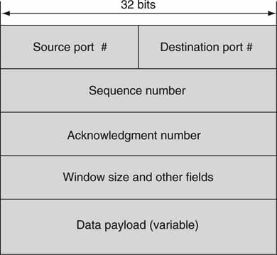
• No address field
• Port numbers used to distinguish application-layer services
• Sequence number
• Acknowledgment ID
• Window size
• Data payload—actual user data such as files
As Figure 6.8 shows, port numbers identify services. Many different TCP connections may exist simultaneously, each associated with a different application. For example, well-known port 21 is dedicated to FTP and 80 to HTTP for Web page access. There are 64K ports available, some assigned to specific services. Registered applications use what are called well-known ports for access.
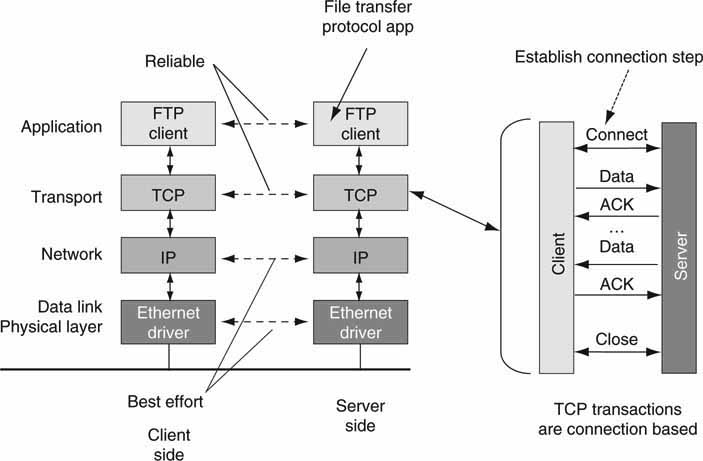
TCP is a connection-oriented protocol. This means that a handshake protocol is used to establish a formal communication between two devices before any payload data are exchanged. End point connections are called sockets. For example, when you are connecting to a Web server, a TCP connection is first established before any Web pages are downloaded. Figure 6.10 illustrates steps needed to move a file between a server and a client using FTP and TCP.
FIGURE 6.10 TCP is connection based and 100 percent reliable.
Concept: CISCO.
TCP connection establishment is a simple three-step sequence and is done only at the beginning of the call. Then file data are moved between the sides. Importantly, TCP requires that every packet be positively acknowledged so that the sender knows with certainty that a sent packet was received without error. Because the setup phase does consume a small amount of time, A/V-centric applications may decide to leave the connection established ready for future use. For short transactions, the setup/close can take >50 percent of the total connection time.
If a packet’s acknowledgment ID is not received within a certain time period, then the suspect packet is re-sent. TCP will reduce its sending rate if too many packets are lost. This behavior helps reduce network congestion. TCP is a good network citizen. Positive acknowledgments and rate control are major features of TCP and have been both a curse and benefit to A/V data transfer performance. Figure 6.11 illustrates an example of sustained TCP performance in the presence of packet loss. Note the aggressive backoff and slow startup. The throughput would be constant only if packet loss was effectively zero. Although an IP packet can carry up to 64KB of payload data, when Ethernet is the underlying link layer, it is wise to limit IP data length to 1,500B—the Ethernet frame payload size. If a data bit error occurs at the frame or packet level, 1,500B of payload is lost for the general case.
FIGURE 6.11 Behavior of TCP in the presence of packet loss.
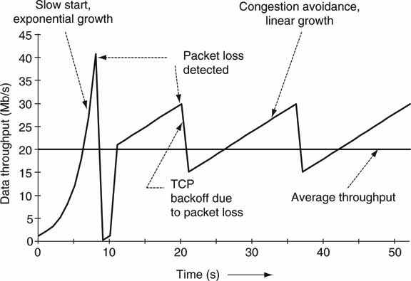
Concept: Cisco
6.1.3.1 The Sliding Window
TCP uses what is called a sliding window approach to manage transmission reliability and avoid congestion, as illustrated in Figure 6.12. There are three kinds of payload data in the vocabulary of TCP:
FIGURE 6.12 TCP’s sliding data window.
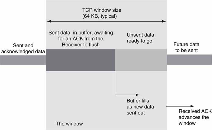
1. Sent and acknowledged (ACK) data packets; the receiver has the data
2. Sent and awaiting an ACK from the receiver; the receiver may not yet have the data
3. Data packets not yet sent
Data that fall into case #2 are governed by the sliding window. In most cases, the TCP window is 64KB, although RFC 1323 allows for a much larger window with a corresponding increase in transfer rates over long-distance links. When the sender transmits a data packet, it waits for the receiver to acknowledge it. All unacknowledged sent data are considered “in the window.” If the window becomes full, 64KB of outstanding data, then the sender stops transmitting until the next ACK is received.
For short-distance hops, the window does not impair performance because ACKs are received quickly. For long-distance transfers (across WANs, satellites), small windows contribute to slow FTP rates because the transmission pipe fills quickly with unacknowledged data. More on this later in the chapter.
Despite some performance problems with TCP, it is the king of the transport layer. How does it compare to User Datagram Protocol (UDP), its simpler cousin? Let us see.
6.1.3.2 UDP Transport
In basic terms, UDP is a send-and-hope method of transmitting data. There are no connection dialogs, acknowledgments, sequence numbers, or rate control; UDP just carries payload data to a receiver port number. A UDP packet is launched over IP and, if all goes well, arrives at the receiver without corruption. UDP is a connectionless protocol compared to TCP being connection based.
Who would want to use UDP when TCP is available? Well, here are a few of UDP’s advantages:
• UDP is very easy to implement compared to TCP.
• It has almost no software overhead and is very CPU efficient.
• It provides efficient A/V streaming (VoIP uses UDP and RTP to carry voice data for a call).
• There is no automatic rate control as with TCP; transmission metering can be set as needed.
• There is minimal delay from end to end.
• It supports point-to-multipoint packet forwarding (IP multicast).
If the network is not congested and application data are somewhat tolerant of an occasional packet loss, then UDP is an ideal transport mechanism. In fact, UDP is the basis for many real-time A/V streaming protocols. When you listen to streaming music at home over the Internet, UDP is often the payload carrier.
When UDP is coupled with custom rate control, it can outperform TCP. Some UDP-based file transfer protocols use TCP only to request a packet resend and set rates. Although TCP is part of the transaction, its use is infrequent and highly efficient. Some A/V streaming applications use error concealment to hide an infrequent missing packet. See Chapter 2 for examples of both UDP- and TCP-based file transfer applications.
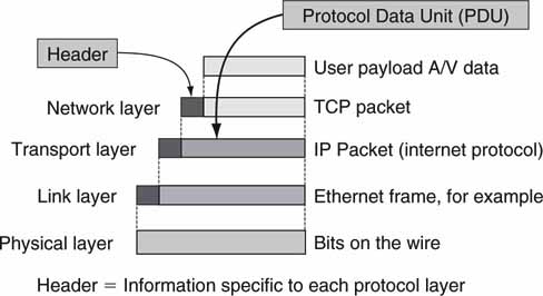
6.1.3.3 Stacking It All Up
The stack is a good way to organize the concepts and interactions of IP-related standards. The peer-to-peer relationship of the layers is an excellent way to divide and conquer a complex set of associations. Figure 6.13 summarizes how packets are encapsulated by the layer above. In the simplest form, each packet type is a header followed by a Protocol Data Unit (PDU). The IETF has set standards for each of these layers and their corresponding packet format. As trillions of packets transit the Internet and private networks each day, the IP stack has proven itself worthy of respect.
FIGURE 6.13 Packet encapsulation.
LANs are built out of the fabric of the stack, but not all LANs are created equal. Next, the VLAN is considered.
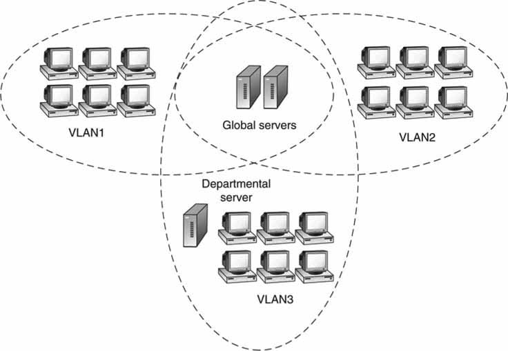
6.2 VIRTUAL LANS
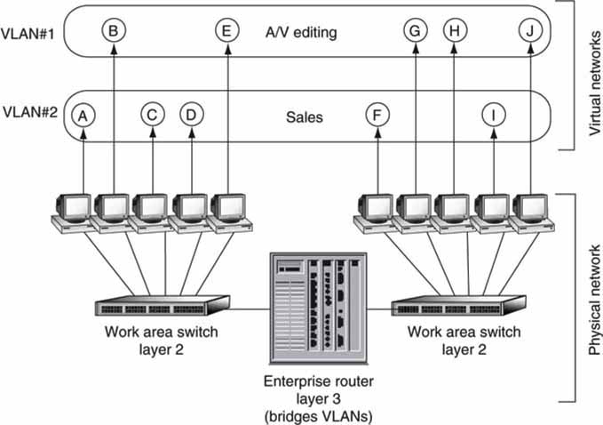
One huge, flat network easily interconnects all attached nodes. At first blush, this may seem like the ideal topology. However, dividing it into smaller subnet domains offers better QoS, reliability, security, and management. Using a VLAN is a practical method to implement the segmentation. With a VLAN, the A/V domain may be on one LAN, sales on a second LAN, human resources on a third, and so on. Segmenting LANs is the ideal way to manage the network resources of each department or domain. Figure 6.14 illustrates the division of LANs. Especially important for A/V applications is the isolation between LANs afforded by VLANs.
FIGURE 6.14 A network of isolated VLANs.
During normal LAN operation, various layer 2 broadcast messages are sent to every member of a LAN. With VLANs, these broadcast messages are forwarded only to members of the VLAN. VLAN node isolation is a key to its performance gain. The IEEE has standardized 802.1Q for VLAN segmentation. The following section covers the layout and advantages of VLANs over traditional LANs.
6.2.1 VLAN Basics
In a traditional Ethernet LAN, nodes (PCs, servers, etc.) connected to the same layer 2 switch share a domain; every node sees all broadcast frames transmitted by every other node. The more nodes, the more contention and traffic overhead are present. LAN QoS falls as the number of nodes increases. To avoid poor performance, the LAN must be decomposed into smaller pieces.
Nodal segmentation can be done by throwing hardware at the problem. Connect one set of stations to switch A, another to switch B, and so on and performance increases. This has the problem that associated nodes need to be in the same proximity. Is there a smarter way to segment a LAN? Yes.
VLANs provide logical isolation in place of physical segmentation. A VLAN is a set of nodes that are treated as one domain regardless of their physical location. A VLAN can span a campus or the world. Stations in VLAN #1 hear other stations’ traffic in VLAN #1, but do not hear stations in other VLANs, including those connected to the same switch. This isolation is accomplished using VLAN tagging (see Figure 6.15). A VLAN tag is a 4-byte Ethernet frame extension (layer 2) used to separate and identify VLANs. Importantly, a VLAN’s data traffic remains within that VLAN and can cross outside only with the aid of a layer 3 switch/router. Segmentation is especially valuable for critical A/V workflows where traffic isolation is needed for reliable networking and achieving a desired QoS.
FIGURE 6.15 VLAN segmentation example.
Concept: Encylopedia of networking and telecommunications.
For example, a layer 2 switch may be configured to know that ports 2, 4, and 6 belong to VLAN #1, whereas ports 3, 5, and 7 belong to VLAN #2, and so on. The switch sends out arriving broadcasts to all ports in the same VLAN, but never to members of other VLANs.
• QoS is improved for A/V VLAN segments.
• An A/V client may have two Ethernet ports, one per VLAN. With two VLAN attachments per device, it is possible to access VLAN #2 if VLAN #1 has failed. This is key to some HA dual pathing methods discussed in Chapter 5.
• Network problems on one VLAN do not necessarily affect a different VLAN. This is needed when the A/V network needs separation from, say, a business LAN.
• A VLAN has more geographical flexibility than with IP subnetting.
VLANs are not the only way to improve performance, security, and manageability. The next section outlines some protocols designed for setting and maintaining QoS levels.
6.3 TCP/IP PERFORMANCE
TCP has built-in congestion control and guaranteed reliability. These features limit the maximum achievable transfer rate between two sites as a function of the advertised link data rate, round trip latency, and packet loss. As discussed earlier, TCP’s sliding window puts a boundary on transfer rates. TCP’s average data throughput is given by the following three principles; the one with the lowest value sets the data rate ceiling.
TCP limitation 1. You cannot go faster than your slowest link.
• If the slowest link in the chain between two communicating hosts is limited to R Kbps, then this is the maximum throughput.
TCP limitation 2. You cannot get more throughput than your window size divided by the link’s round trip time (RTT).
• RFC 1323 does a good job of discussing this limitation, and TCP implementations that support RFC 1323 can achieve good throughput even on satellite links if there is very little packet loss. An RTT of 0.1 s and a window size of 100KB yield a maximum throughput of 1 MBps.
TCP limitation 3. Packet loss combined with long round trip time limits throughput.
• RFC 3155, “End-to-End Performance Implications of Links with Errors,” provides a good summary of TCP throughput when RTT and packet loss are present. In this case the following approximate equation provides the limiting transfer rate in bytes per second.
Throughput limit 1.2 × (Packet_Size)/(RTT × SQRT (packet loss probability)) Note that TCP’s data throughput depends on link bandwidth only for rule #1. Rule #2 limits data throughput due to window size and round trip time (RTT), and rule #3 limits data rate due to RTT and packet loss. Knowing why a transfer is slow gives the hints needed to improve the transfer performance.
These TCP limitations are clearly illustrated in Figure 6.16. The bar graph shows the maximum continuous data throughput achievable under various RTT and packet loss conditions using a SONET OC-3 (155 Mbps) link. The throughput sensitivity to RTT is obvious. Increasing the RTT from 10 to 100 MS decreases the rate by more than 10×! This is precisely why throwing “bandwidth” at a slow file transfer is often a waste of money.
FIGURE 6.16 TCP data throughput versus round trip time (RTT) and loss.
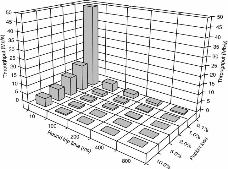
Sensitivity to loss is not as severe. Packet loss going from 0.1 to 1 percent decreases TCP throughput by about a factor of 3×. So, a transit path with 0.1 percent loss and 200 MS of RTT (SF to/from London’s www.bbc.co.uk) would permit data rates ~1 Mbps. This is <1 percent of the maximum achievable data rate. In fact, the transfer rate may be worse if, using the Internet, loss exceeds 0.1 percent or approximately 3 Mbps if at 0.01 percent loss. Of course, the Internet has an undefined QoS, so user beware.
Speedy rates are attainable in local LANs with small RTT (<10 MS) and loss <0.01 percent. So when you are doing system planning, knowing the RTT and loss characteristics of a transmission link will allow you to better predict throughput.
Techniques for improving TCP’s throughput are numerous. Some methods use received error correction (FEC), and some use fine-tuning to adjust the myriad of TCP parameters for more throughput. Figure 6.16 was provided by Aspera, Inc. (www.asperasoft.com). This company offers a method (fasp) using UDP and a return channel to achieve adaptive rate control and realize throughput rates approaching the line rate even in the presence or large RTT values and significant loss. Aspera’s strategy does not use TCP, so both end points must use the non-standardized Aspera technology.
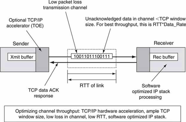
Naturally, the CPU stack processing of TCP/IP packets may also bottleneck performance, despite the efforts to optimize the three factors given earlier. There are countless ways to improve the stack’s software performance, and many TCP processors use clever methods to avoid data copies and so on. Another way to improve TCP’s compute performance is hardware acceleration with a TCP Offload Engine (TOE) card discussed later. A TOE card moves stack processing away from the main CPU to a secondary processor dedicated to TCP/IP processing. Figure 6.17 illustrates chief twiddle factors for improving TCP’s performance.
FIGURE 6.17 Optimizing TCP/IP throughput.
So why do we use TCP at all if it has such limitations? All transfer protocols have less than ideal characteristics for some portion of their operational range. Some researchers have postulated that the relative stability of the Internet is at least partially attributed to TCP’s aggressive back-off gentle slow startup under congestion (Akella 2002). So TCP is a good network citizen. See Chapter 2 for a list of methods to accomplish fast file transfer without using TCP.
6.3.1 Screaming Fast TCP/IP Methods
Researchers at the University of Amsterdam (Antony 2003) did an end-to-end file transfer experiment with the test conditions shown in Figure 6.18. They used high-end servers with 10G Intel Host Bus Adaptor (HBA) cards. These are not TOE cards. The servers ran Linux with specialized TCP stack software called TCP Vegas. One end point was in Amsterdam, and the other was in Geneva. Each 10G Ethernet LAN connected to a STM-64 10-Gbps WAN (SONET) using a Force 10 router. The round trip delay between sites was only 17 MS. Using only CPU TCP processing, the throughput reached 5.22 Gbps (about half of the 10G user payload) after proper tweaking of the TCP window size (socket buffer size was the adjustable parameter).
FIGURE 6.18 High-speed transmission test configuration.
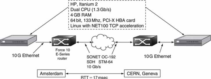
What limited the throughput performance? The researchers believe it was the internal PCI-X bus bandwidth. Also, if the WAN link had any congestion, the rate would have dropped precipitously. User data were R/W to RAM, not to HDD devices, so memory speeds were not an issue. The end device servers are high end and expensive. With a TOE card to accelerate the stack, the performance will increase. The next section discusses TOEs.
6.3.2 TCP Offload Engines (TOEs)
A TOE card is a server or workstation plug-in card (PCI-X or similar, or on a motherboard) that offloads the CPU-intensive TCP/IP stack processing. To obtain the fastest iSCSI, NAS, or file transfers, you may need a TOE card. The card has an Ethernet port, and all TCP/IP traffic passes through it. At 100 Mbps Ethernet speeds, most CPUs can handle the processing overhead of TCP. A generally accepted rule of thumb is that a CPU clock of 1 Hz can process the TCP overhead associated with transferring data at 1 bps. With the advent of 10G Ethernet, server and host CPUs are suffocating while processing the TCP/IP data packets.
The research firm Enterprise Strategy Group (www.enterprisestrategygroup.com, Milford, MA) has concluded that “implementing TCP off-load in hardware is absolutely a requirement for iSCSI to become mainstream. TCP is required to guarantee sequence and deal with faults, two things block-oriented storage absolutely requires. Running TCP on the server CPU will cripple the server eventually, so bringing the function into hardware is a must.” TOE cards are used for some 1G and most 10G iSCSI host ports. Many iSCSI storage vendors use TOE cards.
6.3.3 A Clever Shortcut to TCP Acceleration
WAN transfer-speed acceleration is a proven concept given a WAFS appliance (see Chapter 3B), or similar, at each end point. But, can TCP be accelerated with a WAFS-like appliance located at only one end point? Surprisingly, yes. Researchers at Caltech, Pasadena (Cheng Jin 2004) have invented methods, collectively termed FastTCP, to accelerate TCP using only an appliance at the sending side. The receiving side(s) uses unmodified, industry standard TCP.
Using a combination of TCP-transmitted packet metering, round trip delay measurement, and strategies to deal with packet loss, a single appliance can achieve up to 32× throughout compared to no acceleration. The methods really shine when the end-to-end path has >100 Ms delay, >0.1 percent loss, and the pipe is large, >5 Mbps. A link with these characteristics is often called a long fat pipe.
FastTCP has been implemented by FastSoft (www.fastsoft.com) in its Aria appliance. FastTCP currently holds the world’s record for TCP transfer speeds with a sustained throughput of 101 Gbps. Imagine what FastTCP can do for transferring large video files over long distances using lossy Internet pipes. Plus, Aria supports up to 10,000 simultaneous connections: think Web servers.
6.4 THE WIDE AREA NETWORK (WAN)
A WAN is a physical or logical network that provides communication services between individual devices over a geographic area larger than that served by local area networks. Connectivity options range from plain-old telephone service (POTS) to optical networking at 160 Gbps rates (proposed). Terms such as T1, E3, DS0, and OC-192 are often referred to in WAN literature, and frankly this alphabet soup of acronyms is confusing even to experts. There is no need to sweat like a stevedore when parsing these terms. See Appendix F for simple definitions and relationships of these widespread terms. Some of the links discussed in the appendix are used commonly to connect from a user’s site to a Telco’s office. Other links are dedicated to the generic Telco’s internal switching and routing infrastructures. Usually, a WAN is controlled by commercial vendors (Telcos and the like), whereas a LAN is controlled by owners/operators of a facility or campus network. The QoS of the network depends not only on the type, but who controls it.
The four main criteria for segmenting wide area connectivity are
• Topologies: Switched and non-switched (point to point, mesh, ring)
• Networks: Private and public
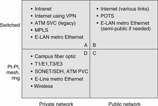
Figure 6.19 segments these methods into four quadrants. An overview of topologies follows.
FIGURE 6.19 Wide area transport-type classifications.
6.4.1 WAN Connectivity Topologies
Each of the four types in Figure 6.20 may be used for general data communications, file transfer, storage access, and live A/V streaming. Figure 6.20 expands on Figure 6.19. Each has trade-offs in the areas of QoS, cost, reliability, security, and so on. The trade-offs are not covered in detail, but some consideration will be given to A/V-specific issues.
FIGURE 6.20 Wide area topologies.
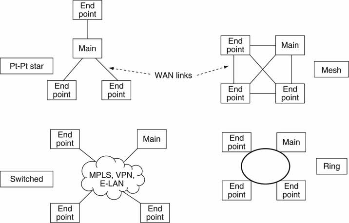
The point-to-point form is the most common type of connectivity. One example of this may be remote A/V sources (say, from three sports venues) all feeding live programming to a main receiver over terrestrial or satellite links. Many businesses have remote offices configured via a point-to-point means.
The mesh allows for peer-to-peer communications without going through a central office for routing. Depending on the geographic locations of the end points, a mesh may not make economic sense. In general, the mesh has been replaced by switched networks. The complexity of a mesh rises as the square of the number of nodes.
The ring is a common configuration implemented by Telcos in a city or region. Using SONET, for example, a ring may pass by big offices or venues. Using short point-to-point links, the ring may be connected to nearby end points. Rings are often built with two counter rotating paths to provide for fault tolerance in the event that one ring dies. Many Telcos offer MAN services often based on ring technology.
Finally, there are switched topologies. The most common are
• Internet based (DSL, cable, other access), VPN or not
• Carrier Ethernet—E-LAN
• Multiprotocol Label Switching (MPLS)
Switched methods do not always offer as good a QoS as the other methods. Why? Switching introduces delay, loss, and jitter often not present in the others. Of course, WAN switching can exhibit excellent QoS, but only for selected methods such as MPLS and some Carrier Ethernet networks. MPLS is explained later in this chapter.
6.4.2 Network Choices
Figure 6.19 divides WAN network choices into public and private. WANs are available through Telcos and other providers. They are available to anyone who wants to buy a service connection. Normally, anyone on a given system can communicate to any other member. Quad A lists the most common enterprise WAN configurations. Nodes communicate over a managed service switched network. Users are offered a Service Level Agreement (SLA) that sets the QoS levels. Quadrant B shows the most common public switched networks. These are typically not managed, so the QoS level may be low. Quadrant D as a point-to-point system potentially offers excellent QoS for all types of A/V communications.
Whether a network is considered public or private, Telcos and other service providers can offer the equipment and links to build the system. The distinction between public and private is one of control, security, QoS, and access more than anything else. Given the right amount of packet reliability and accounting for delay through a network, any of the quadrants will find usage with A/V applications.
The Video Services Forum (VSF, www.videoservicesforum.org) is a user group dedicated to video transport technologies, interoperability, QoS metrics, and education. It publishes guidelines in the following areas:
• Multicarrier interfacing for 270 Mbps SDI over SONET (OC-12)
• Video over IP networks
• Video-quality metrics for WANs
• Service requirements
The VSF sponsors VidTrans, an annual conference where users, Telcos, and equipment vendors gather to share ideas and demonstrate new A/V-networked products.
Another topic of interest to A/V network designers is the Carrier Ethernet. The next section outlines this method.
6.5 CARRIER ETHERNET (E-LAN and E-LINE)
Ethernet has continually evolved to meet market needs. It was initially developed as a LAN. Over the years it has morphed from 10 Mbps data rate to a soon-to-be 100 Gbps. Ethernet has staying power, and other layer 2 technologies have taken a back seat to its network dominance. Recently, Ethernet has been applied to metropolitan area networking (MAN) and even global level networking. This level of switching and access is termed Carrier Ethernet. This enables a seamless interface between a campus LAN and another campus LAN many miles away.
The Metro Ethernet Forum (MEF) has defined the following two standardized service types for Carrier Ethernet:
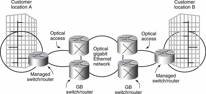
• E-LAN: This multipoint-to-multipoint transparent LAN service offers switched connectivity between nodes in a layer 2 Carrier Ethernet network. Figure 6.21 shows an example.
FIGURE 6.21 Example of Carrier Ethernet E-LAN configuration.
• E-Line: This is a virtual private line between two end points. There is no switching, and each line is statically provisioned.
Another dimension of value is geographical reach. The MEF is working to standardize the interconnection of Ethernet networks operated by different service providers, thus enabling a consistent user experience across vendors and distance. Carrier Ethernet provides the necessary QoS levels required for nodes to be seamlessly connected over a common infrastructure.
Regarding reliability, Carrier Ethernet can rapidly detect and recover from node, link, or service failures. Recovery from failures occurs in less than 50 milliseconds. This capability meets the most demanding availability requirements. For a video file transfer application, a 50 Ms reroute delay would not affect reliable delivery. Even for best-effort video streaming, only a few frames would be lost (not counting the time to resync the video). The missing frames may be concealed if needed.
Finally, Carrier Ethernet is centrally managed using standards-based vendor-independent tools. The advantages are as follows:
• Provision services rapidly
• Diagnose connectivity-related problems reported by a customer
• Diagnose faults in the network at any point
• Measure the performance characteristics of the service
Infonetics Research forecasts that worldwide Ethernet services revenue will be $22.5 billion in 2009. Clearly, Carrier Ethernet is a viable switched network service for the media enterprise.
6.6 UNDERSTANDING QUALITY OF SERVICE FOR NETWORKS
The heart and soul of high-quality, digital A/V networking is the QoS4 metric: low delay, low jitter, controlled bandwidth, low packet loss, and high reliability. Hand-wringing is common over maintaining QoS levels. Who sets them, how can they be guaranteed, and when are they out of limits? These are common concerns. Link QoS may be specified in a contract called a Service Level Agreement (SLA). Service suppliers provide SLAs whenever contracted for LAN or WAN provisioning. The elements of an SLA are useful criteria for any network design. QoS-related items are as follows:
• Delay. Also called latency, this is the time it takes a packet to cross the network through all switches, routers, and links. Link delays are never good, and the absolute value of an acceptable delay depends on use. Control signaling, storage access, file transfer, streaming (especially live interviews), and so on—each has different acceptable values. Delay may be masked by using A/V prequeuing and other techniques. Control has the strictest requirement for low delay and may be less than one line of video for some applications. However, for most applications, a control signal delay less than ~10 ms (less than half a frame of video) is sufficient. For LANs a 10 ms maximum delay is well within range of most systems.
• Jitter. This is the time variation of delay. Jitter is difficult to quantify, but knowing the maximum expected value is important.
• Controlled bandwidth. Following are four common ways (some or all) to guarantee data rate:
1. Overprovision the links with sufficient bandwidth headroom. Meter the ingress data rate to known values (e.g., 5 Mbps max).
2. Do loading calculations for each link and switch to guarantee no switch congestion or link overflow at worst-case loading.
3. Use reservation protocols to guarantee link and network QoS.
4. Eliminate all IP traffic that does not have predictable data rates so that uncontrolled FTP downloads of huge files are not allowed over specified LAN segments. A rate shaping gateway may be used to tame unpredictable IP streams.
• Packet loss. The most common cause comes from congested switches and routers. A properly configured switch will not drop any packets, even with all ports at 100 percent capacity. Of course, traffic engineering must guarantee that ports are never overloaded. A/V clients that are good network citizens will always control their network I/O and thus help prevent packet congestion. It can be very difficult to eliminate data bursts that can cause congestion and packet loss downstream.
• Reliability. This topic is considered at length in Chapter 5 but is typically one of the most important elements of a SLA.
It is a good plan to work with A/V equipment providers that understand the subtleties of mission-critical networking and guaranteed QoS. See Chapter 2 for an illustration of network-related QoS metrics in action.
The Internet is a connectionless packet switched network, and all services are best effort. In contrast, leased lines and SONET are connection oriented, and data are delivered in predictable ways. Guaranteeing the QoS for a general Internet connection is nearly impossible. The Internet carriers do not agree on how to set and manage QoS criteria, someone has to pay for the extra level of service, and there is little motivation to change the status quo. There are specialized networks where the provider guarantees QoS using Multiprotocol Label Switching (MPLS) and Carrier Ethernet. This discussion does not make a distinction between class of service (CoS) and QoS, although they are different in principle. A CoS is a routing over a network path with a defined QoS. Incidentally, MPLS is designed to be network layer independent (hence, the name multiprotocol) because its techniques are applicable to any network layer protocol, but IP is the most common case.
QoS types can be broadly defined as soft or hard. A soft QoS has loose bandwidth guarantees, is statistically provisioned, and is defined in a hop-by-hop way. Hard QoS has (guaranteed rate rates,) bounded delay and jitter, deterministic provisioning, and is defined end to end. Hard QoS connections are best for professional streamed video applications. What are the chief categories for QoS control? Here are some commonly accepted techniques:
• Congestion management. These methods reduce or prevent congestion from occurring.
• QoS classification techniques. IP packets are each marked (tagged) and directed to queues for forwarding. The queues are prioritized for service levels.
• QoS reservation techniques. Paths are reserved to guarantee bandwidth, delay, jitter, and loss from end to end.
Let us consider each one of these in brief.
6.6.1 Congestion Management
TCP has built-in congestion management by detecting packet loss and backing off by sending fewer packets and then slowly increasing the sending rate again (Figure 6.11). TCP is a major reason for the inherent stability and low congestion loss of the Internet. Within the network, routers sense congestion and may send messages to other IP routers to take alternate paths. Also, some routers may smooth out bursty traffic and reduce buffer overflows along the path. A router may use the Random Early Detection (RED) method to monitor internal buffer fullness and drop select packets before buffers overflow. Any congestion for critical A/V applications is bad news. High-quality streaming links cannot afford congestion reduction—they need congestion avoidance. File transfer can live with some congestion because TCP will correct for lost packets.
6.6.2 QoS Classification Techniques
Methods for QoS classification techniques are based on inspecting some parameter in the packet stream to differentiate and segment it to provide the desired level of service. For example, if the stream is going to a well-known UDP port address (say a video stream), then the router may decide to give this packet a high priority. Sorting on port numbers is not the preferred way to classify traffic, however; it breaks the law of independence of stack layers. The generally accepted classification methods in use today are based on tags. The three most popular means are as follows:
• Ethernet frame tagging. This is based on an IEEE standard (802.1D-1998) for prioritizing frames and therefore traffic flows. It has limited use because it is a layer 2 protocol and cannot easily span beyond a local LAN. For A/V use in small LANs, this type of segmentation is practical, and many routers and switches support it.
• Network level ToS tagging. The type of service (ToS) is an 8-bit field in every IP packet used to specify a flow priority. This layer 3 field has a long history of misuse but was finally put to good use in 1998 with the introduction of IETF’s Differentiated Services (Diffserv) model as specified by RFC 2475. Diffserv describes a method of setting the ToS bits (64 prioritized flow levels) at the edge of the network as a function of a desired flow priority, forwarding each prioritized IP packet within the network (at each router) based on the ToS value, and traffic shaping the streams so that all flows meet the aggregate QoS goals. Diffserv is a class of service method to manage data flows. It is a stateless methodology (connectionless) and does not enforce virtual paths as MPLS does.
• MPLS tagging. This technique builds virtual circuits (VCs) across select portions of an IP network. Virtual circuits appear as circuit switched paths, but they are still packet/cell switched. VCs are called label switched paths (LSPs). MPLS is an IETF-defined, connection-oriented protocol (see RFC 3031 and others). It defines a new protocol layer, let us call it “layer 2.5,” and it carries the IP packets with a new 20-bit header, including a label field. The labels are like tracking slips on a pre-addressed envelope. Each router inspects the label tags and forwards the MPLS packet to the next router based on a forwarding table. Interestingly, the core MPLS routers do not examine the IP address, only the label. The label carries all the information needed to forward IP packets along a path across a MPLS-enabled network. Paths may be engineered to provide for varying QoS levels. For example, a path may be engineered for low delay and a guaranteed amount of bandwidth. MPLS operation is outlined in a later section.
These tagging methods are used in varying proportions in business environments and by Internet providers in the core of their networks. Several companies offer MPLS VPN services. A/V applications, including streaming, critical file transfers, storage access, and real-time control, can benefit from tag-enabled networks. Diffserv and MPLS are sophisticated protocols and require experts to maintain the configurations. Routers also need to be Diffserv and/or MPLS enabled. MPLS and Diffserv may indeed work together, as there is considerable synergy between the two methods. There is more discussion on these two methods in following sections.
6.6.3 QoS Reservation Techniques
Carrier Ethernet and MPLS virtual circuits can guarantee a QoS level while traversing across a broad network landscape. Each can carry IP packets as payload. Before routers pass any cells or packets, the QoS resources should be reserved. There are several ways to set up a virtual path with guarantees. One is to use the Resource Reservation Protocol (aptly named RSVP, RFC 2208, and others). RSVP is an out-of-band signaling protocol that communicates across a network to reserve bandwidth. Every router in the network needs to comprehend RSVP. It finds application in enterprise intranets and in conjunction with MPLS and Carrier Ethernet to reserve path QoS.
Diffserv is a simpler, practical way to forward packets via what are called per-hop-behaviors (PHBs). Hops are defined (by the IETF) with different QoS metrics, such as minimum delay, low loss, or both. When a packet enters a router, its tag is inspected and processed according to the PHB it is assigned to. Admittedly, it is more concerned with class of service than QoS, a subtle distinction.
6.6.4 The QoS Pyramid
Figure 6.22 illustrates the QoS pyramid. At the top of the pyramid is the trusty point-to-point link. There is no packet switching or sharing of bandwidth—it offers premium service at the sacrifice of self-addressed routing flexibility. The SDI (or equivalent) link falls here.
FIGURE 6.22 The QoS pyramid.
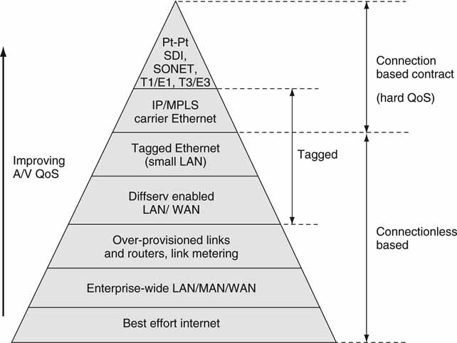
At the bottom is the Wild West of the Internet—the father of best effort service with routing (addressability) as its number one asset. All the other choices in the pyramid are specialized means to guarantee QoS to various degrees. Note that some of the methods are connection based, so a contract exists between end points; whereas others are connectionless with no state between end points. This is independent of the fact that layer 4 (TCP) may establish a connection over IP as needed. Some of the divisions may be arguable, but in general going up the pyramid provides improved QoS metrics.
6.6.5 MPLS in Action
Before we leave QoS, let us look at a simple MPLS-enabled network. As mentioned, MPLS is a connection-oriented protocol, so a contract exists between both ends of a MPLS network path. Figure 6.23 shows the chief elements of such a network. It is link layer independent. Standard IP packets enter the label edge routers (LER) for grooming, CoS classification (usually <8 classes defined, although more are available), and label attachment. MPLS packets traverse the network, routed by label switched routers (LSR).
FIGURE 6.23 A MPLS routing environment.
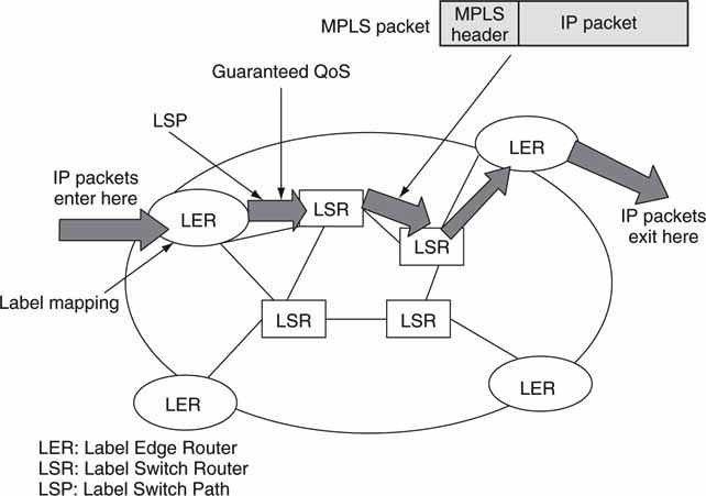
The label is used to route the MPLS packets at each LSR and not the IP address. Packets follow a label switched path (LSP) to the designation LER where the label is striped off as it enters a pure IP routed network. LSPs may be engineered for a range of QoS metrics. MPLS networks are becoming more common and are used in Internet carrier core networks, as offered by Telcos for private networks and for enterprise intranets. Expect to see MPLS applied to A/V applications, as it has a great combination of defined QoS levels and support for IP.
6.7 IT’S A WRAP—SOME FINAL WORDS
Networking is the heart and soul of IT-based media workflows. Just a few years ago, network performance was not sufficient to support professional A/V applications. Today, with proper care, LAN, WAN, and Carrier Ethernet are being used to transport A/V media and control messaging with ample fidelity. MPLS-, Carrier Ethernet-, and Diffserv-enabled connectivity offer good choices for high-quality networking with performance guarantees. With IP networking performance and availability ever increasing, A/V transport is a common occurrence. True, dedicated video links will be with us for some years to come, but A/V-friendly networking is taking more and more of the business that was once the province of specialized A/V suppliers and technology.
1 It is possible that switch forwarding tables may change after a power failure or some network update, so there is no guarantee that a given L2 forwarding path between selected end points will be permanent.
2 An undecillion is 1036.
3 NAT is often referred to as IP masquerading.
4 QoS can be applied to services of all types—networking, application serving, storage related, and so on. Each of these domains has a set of QoS metrics. For this section, networking QoS is the focus.
REFERENCES
Akella, A., et al. (2002). Selfish Behavior and Stability of the Internet: A Game-Theoretic Analysis of TCP. Proceedings of the 2002 ACM Conference on Applications, Technologies, Architectures, and Protocols for Computer Communications, 117–130.
Antony, A., et al. (October 23, 2003). A New Look at Ethernet: Experiences from 10 Gigabit Ethernet End-to-End Networks between Amsterdam and Geneva. The Netherlands: University of Amsterdam.
Jin, C., Wei, D. X., & Low, S. H. (March 2004). TCP FAST: Motivation, Architecture, Algorithms, Performance http://netlab.caltech.edu. Proceedings of IEEE Infocom.
DiMarzio, J. (April 2002). Teach Yourself Routing in 24 Hours Sams. New Jersey: Upper Saddle River.
Jang, S. Microsoft Chimney: The Answer to TOE Explosion? Margalla Communications, www.businessquest.com/margalla/, 8-19-03.
Darren, Spohn. (September 2002). Data Network Design (3rd ed.). NYC, NY: McGraw-Hill Osborne Media.
Stallings, W. (2003). Computer Networking with Internet Protocols. London, UK: Addison-Wesley.
Stevens, R. (1994). TCP/IP Illustrated, volume 1. London UK: Addison-Wesley.