Crossflow Behavior and the Determination Reservoir Parameters by Drawdown Tests in Multilayer Reservoirs
Abstract
The crossflow behavior and its influence on transient well tests are studied when several layers are perforated and produce with a fixed total rate and a common wellbore pressure. Using the semipermeable wall model, an approximate theoretical expression for the crossflow is obtained and compared with the simulation results. The physical reasons for the formation of crossflow and its characters are explained. The relationship between crossflow and the permeability of shales between layers are shown. A well test procedure is suggested, which can be used to determine the kh value for each layer and the permeability of the shales between layers. By comparing the results with the numerical simulation, it is shown that reasonable approximate parameters of the multilayer reservoir can be obtained by using a two-layer model to n-layer cases. More accurate parameters of the multilayer reservoir can be obtained by using the numerical simulation method.
Keywords
Multilayer reservoir; Crossflow; Drawdown test; Numerical simulation; Interpretation method
4.1 Assumption and Mathematical Expression of the Problem
In Chapter 2, we studied the crossflow behavior and its influence on drawdown and buildup tests in a partially perforated two-layer reservoir. A new well test method was suggested, which can be used to determine not only the productivity of each layer, but also the diffusivity ratio of the two layers and the vertical resistance of the shale between the two layers.
In this chapter, we will extend the work of Chapter 2. The problem studied here is the behavior of wellbore pressure and crossflow in an n-layer reservoir when several layers, neighboring each other, produce fluid together with a fixed total rate. A new well test method is suggested. By using the results of the new well tests and the simple calculation method or computer simulation, the kh value of each layer, the diffusivity ratio between layers and the resistance of the shales can be determined.
The following assumptions are used in this work: The n-layer reservoir is homogeneous and infinite (Fig. 4.1). The low permeable shales between layers are homogeneous with negligible thickness, the reservoir is filled with a slightly compressible fluid, gravity can be neglected, and the semipermeable model can be used to approximate the actual reservoir.
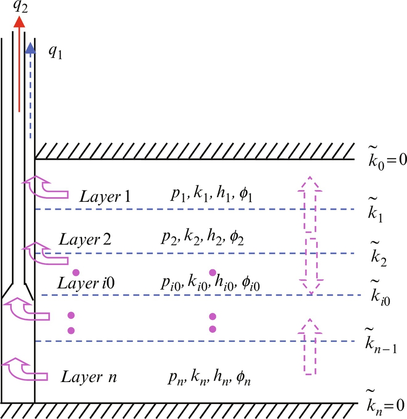
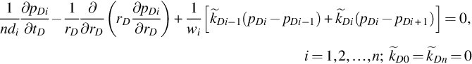
Suppose a well is drilled at an infinite reservoir. Layers 1 to i0 produce with fixed rate q1, and Layers ![]() to n produce with fixed rate q2. The problem can be expressed as follows:
to n produce with fixed rate q2. The problem can be expressed as follows:


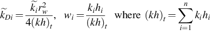
where ![]() ,
, ![]() , and c is compressibility. Using the following dimensionless expressions,
, and c is compressibility. Using the following dimensionless expressions,

Problem Eqs. (4.1)–(4.4) becomes
Set
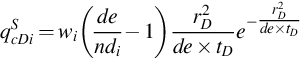
Define the dimensionless crossflow velocity vcDi of layer i as
and the area crossflow rate qcDi as
We found that the crossflow phenomenon can be expressed more clearly by using qcDi.
4.2 The Unsteady Flow Behavior in Drawdown and Buildup Tests When Partial Layers Produce with Crossflow
It was shown that there are three reasons for crossflow in a multilayer reservoir filled with a single-phase fluid as shown in Chapter 1: (1) different boundary pressures for different layers; (2) different diffusivities for different layers; (3) a nonproportional permeability change with position for different layers.
Because of the assumption of a homogeneous reservoir, the third reason for crossflow does not exist here. We shall examine the crossflow caused by different boundary pressures and different diffusivities for different layers.
In an infinite, homogeneous, and two-layer reservoir, there is crossflow caused by the first two reasons when one layer is perforated and produces with a constant rate. The behavior of this crossflow is discussed in detail in Chapter 2. It is shown that the two parts of the area crossflow rate caused by these two factors will increase with time at an early producing time. The crossflow rate caused by different boundary pressures links with well and gradually approaches the steady state. The area crossflow rate caused by different diffusivities gradually behaves like an unchanged wave moving away from the well. This is the distinguishing feature of the area crossflow rate caused only by different diffusivities between layers.
For the purpose of studying the crossflow behavior when only some layers produce and in order to determine the physical parameters of the producing layers and the semipermeable walls, we use a standard difference method and simulate some cases on the computer.
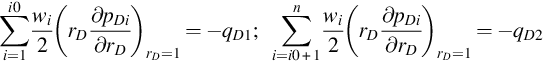
The simulation results for a four-layer reservoir will be described below, which can be used to explain the crossflow phenomenon and indicate how to get the parameters of the multilayer reservoir. In the simulation, the boundary condition ![]() is replaced by an approximate condition:
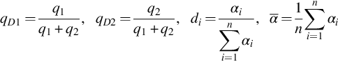
is replaced by an approximate condition: ![]() . The two sections of the well—Layers 1 to i0 and Layers i0+1 to n—produce with a constant rate
. The two sections of the well—Layers 1 to i0 and Layers i0+1 to n—produce with a constant rate ![]() and
and ![]() respectively for dimensionless time
respectively for dimensionless time ![]() and then shut down. The duration of shutdown is also 107. The dimensionless productivities of the layers are wi=0.4, 0.4, 0.1, and 0.1. Several cases were simulated for different diffusivities and semipermeabilities.
and then shut down. The duration of shutdown is also 107. The dimensionless productivities of the layers are wi=0.4, 0.4, 0.1, and 0.1. Several cases were simulated for different diffusivities and semipermeabilities.
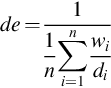
Set
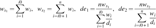
![]() and de1 can be treated as the productivity and effective diffusivity of section 1 (Layers 1 to i0),
and de1 can be treated as the productivity and effective diffusivity of section 1 (Layers 1 to i0), ![]() and de2 as the productivity and effective diffusivity of section 2 (Layers i0+1 to n). The wellbore pressures of the two sections are expressed by
and de2 as the productivity and effective diffusivity of section 2 (Layers i0+1 to n). The wellbore pressures of the two sections are expressed by ![]() and
and ![]() respectively.
respectively.
4.2.1 Behavior of Wellbore Pressure
Figs. 4.2–4.4 show the wellbore pressure change in drawdown and buildup when i0 is equal to 1, 2, and 3 respectively. The buildup curve is the mirror image of the drawdown curve, which is similar to the case when one layer is perforated in a two-layer reservoir, described in Chapter 2. The ![]() versus ln (1+tD) curve has two straight lines. The slope of the first straight line is
versus ln (1+tD) curve has two straight lines. The slope of the first straight line is ![]() ;
; ![]() can be determined by this slope. The slope of the second straight line is
can be determined by this slope. The slope of the second straight line is ![]() ; from it, the total productivity of the reservoir can be determined.
; from it, the total productivity of the reservoir can be determined.


In the first straight line period, ![]() , the wellbore pressure of Section 4.2 is equal to zero, as though the semipermeability between the two sections were zero. In the second straight line period,
, the wellbore pressure of Section 4.2 is equal to zero, as though the semipermeability between the two sections were zero. In the second straight line period, ![]() is a straight line parallel to
is a straight line parallel to ![]() , so
, so ![]() becomes constant. From Fig. 4.3 it can also be seen that the semipermeability change within the sections can cause some changes in wellbore pressure, while the semipermeability between the two sections does not change. However, the wellbore pressure is quite unresponsive to the semipermeability change within sections. Compared to Fig. 4.5, we see that the steady value of
becomes constant. From Fig. 4.3 it can also be seen that the semipermeability change within the sections can cause some changes in wellbore pressure, while the semipermeability between the two sections does not change. However, the wellbore pressure is quite unresponsive to the semipermeability change within sections. Compared to Fig. 4.5, we see that the steady value of ![]() is mainly determined by the semipermeability between the two sections, though the semipermeabilities within the section may have some influence. The reason is, since fluid can exchanges through the wellbore very easily, the resistance of the semipermeable wall to flow within sections cannot play a full role (assume there is no skin factor). If severe skin factors exist, and fluid cannot exchange easily through the wellbore, then the semipermeabilities within sections will have a large influence on the steady value of
is mainly determined by the semipermeability between the two sections, though the semipermeabilities within the section may have some influence. The reason is, since fluid can exchanges through the wellbore very easily, the resistance of the semipermeable wall to flow within sections cannot play a full role (assume there is no skin factor). If severe skin factors exist, and fluid cannot exchange easily through the wellbore, then the semipermeabilities within sections will have a large influence on the steady value of ![]() , especially when the semipermeabilities are not large.
, especially when the semipermeabilities are not large.

4.2.2 Behavior of the Area Crossflow Rate
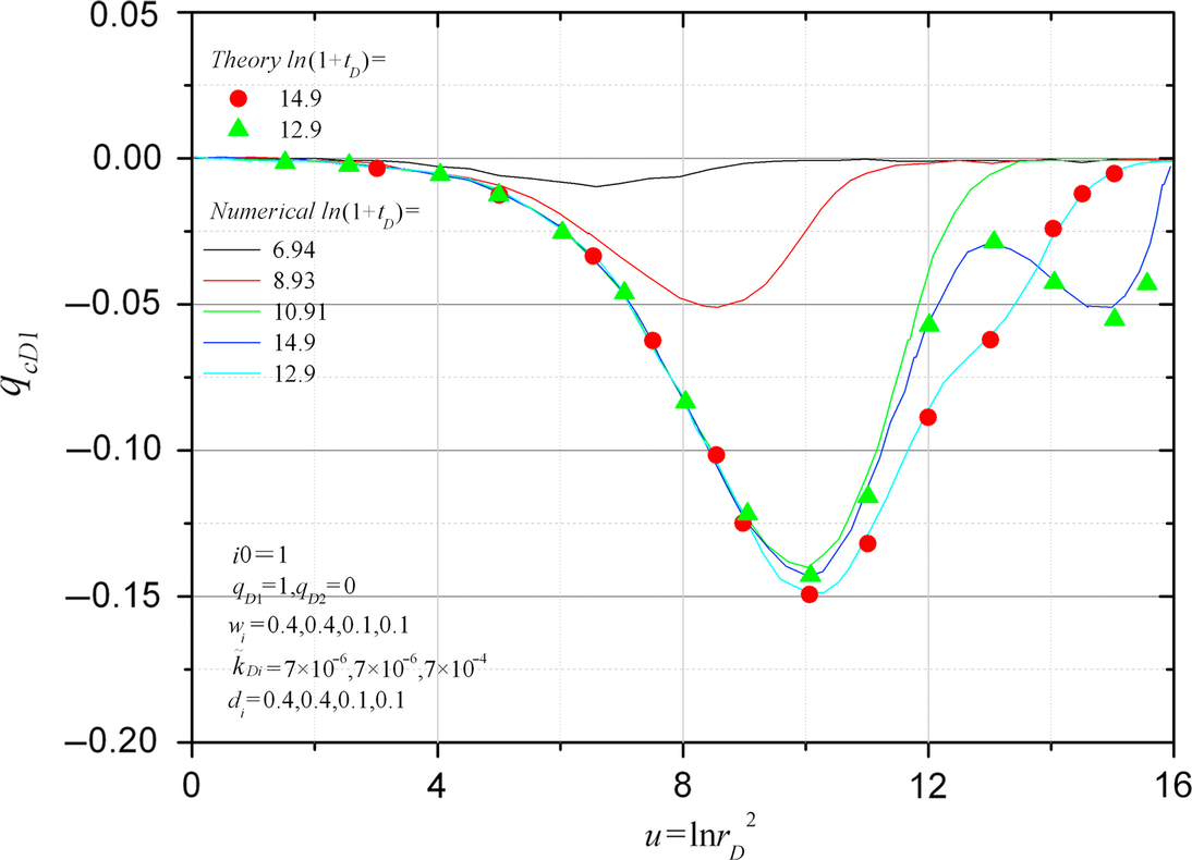
Figs. 4.6–4.8 show the distributions of the area crossflow rate of Layers 1–3 for ![]() at different times. It can be seen that in the early period, qcDi increases with time and the peak point moves outward. Afterward, the one-peak curve becomes a two-peak curve; the peak near the well becomes stable while the peak away from the well moves outward like an unchanged wave. The peak near the well represents the crossflow part caused only by different boundary pressures; the peak far from the well and moving outward with time represents the crossflow part caused by different diffusivities for different layers. We take
at different times. It can be seen that in the early period, qcDi increases with time and the peak point moves outward. Afterward, the one-peak curve becomes a two-peak curve; the peak near the well becomes stable while the peak away from the well moves outward like an unchanged wave. The peak near the well represents the crossflow part caused only by different boundary pressures; the peak far from the well and moving outward with time represents the crossflow part caused by different diffusivities for different layers. We take ![]() in the calculation. This means that all the layers have the same thickness. It can be seen that the crossflow obtained by Layer 1 near the well is given up by Layers 2, 3, and 4. In the region far from the well, where the crossflow is caused mainly by different diffusivities, the crossflow to Layers 1 and 2 is given up by Layers 3 and 4. Thus, the crossflow in Layer 2 is positive in some places and negative in others. The area crossflow rate qcD4 for Layer 4 is almost exactly the same as qcD3, shown in Fig. 4.8, so it is not drawn out. Because of the large value of semipermeability
in the calculation. This means that all the layers have the same thickness. It can be seen that the crossflow obtained by Layer 1 near the well is given up by Layers 2, 3, and 4. In the region far from the well, where the crossflow is caused mainly by different diffusivities, the crossflow to Layers 1 and 2 is given up by Layers 3 and 4. Thus, the crossflow in Layer 2 is positive in some places and negative in others. The area crossflow rate qcD4 for Layer 4 is almost exactly the same as qcD3, shown in Fig. 4.8, so it is not drawn out. Because of the large value of semipermeability ![]() , the behavior of Layers 3 and 4 should almost be the same.
, the behavior of Layers 3 and 4 should almost be the same.
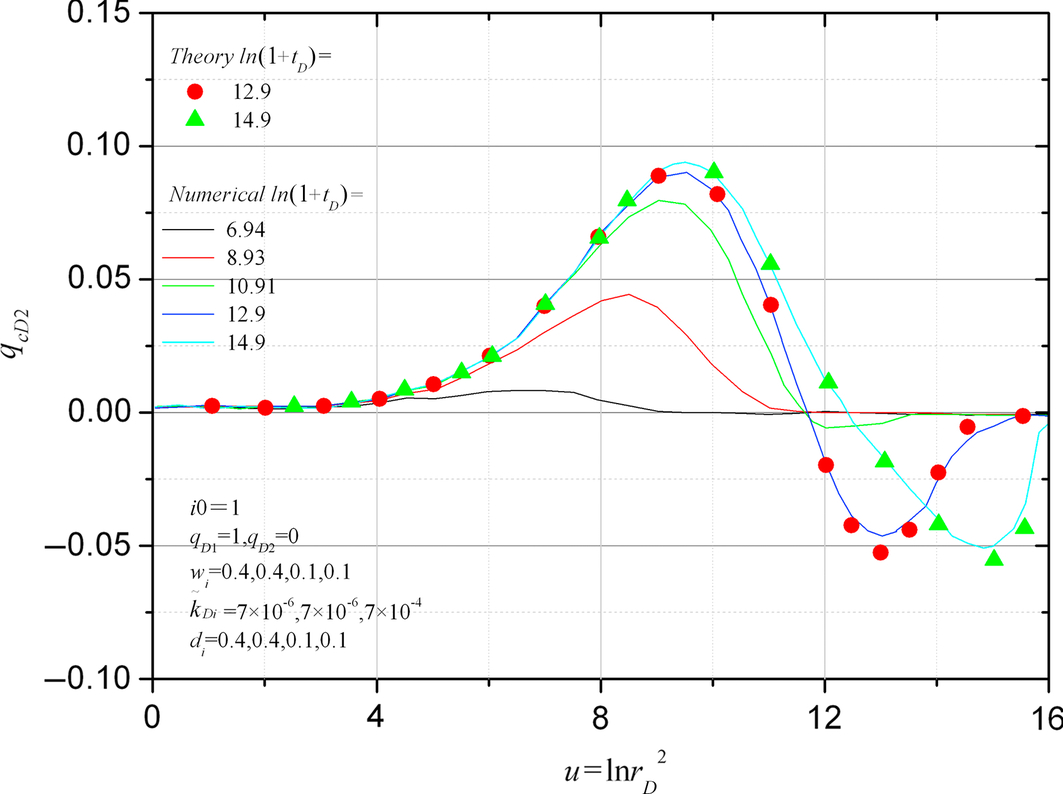
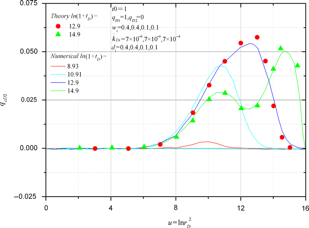
Figs. 4.9–4.11 show the distribution of the area crossflow rate in Layers 1 to 3 at different times when ![]() . Because
. Because ![]() is very large, the distributions of qcD3 and qcD4 are almost the same as for the case of
is very large, the distributions of qcD3 and qcD4 are almost the same as for the case of ![]() .
. ![]() is relatively small, so qcD1 develops slower than qcD2 does, though they are similar to each other.
is relatively small, so qcD1 develops slower than qcD2 does, though they are similar to each other.
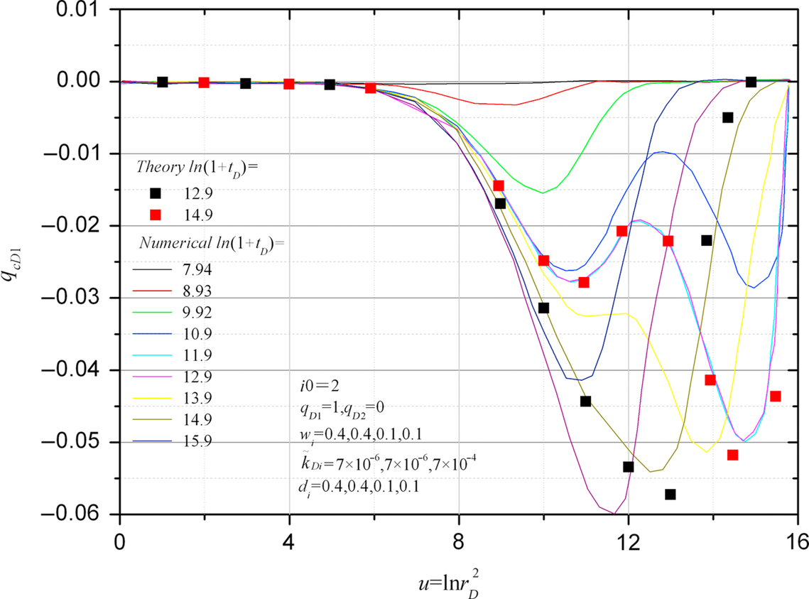
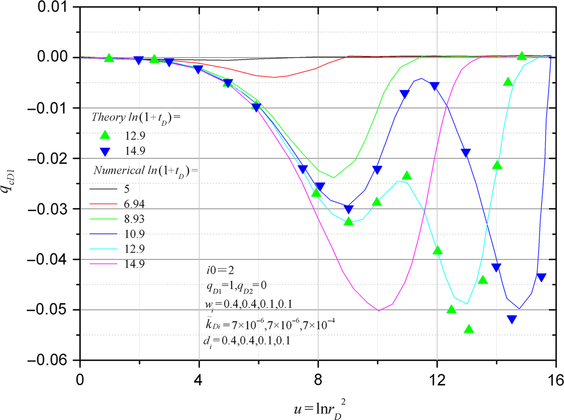

In Chapter 3, a detailed study is given for the crossflow caused only by different diffusivities. According to it, the area crossflow rate, caused only by different diffusivities, can be expressed as
in the second straight line period, where
is the effective dimensionless diffusivity of the reservoir. Eq. (4.13) is a one-peak curve, and the peak value occurs at

With an increase in time, the peak will move outward. From Eq. (4.13), the peak value qcDiS can be obtained:

It is easy to verify that the second peak, which moves outward with time, is approximately expressed by Eq. (4.13).
In Appendix C, a solution is given to the crossflow caused by different boundary pressures. The comparison in figures shows that the theoretical solution agrees quite well with the simulation results.
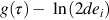
4.2.3 Behavior of Function g(tD)
Fig. 4.5 shows the change of function g(tD), where

It can be seen that for different qD1 and qD2, function g(tD) increases along a straight line with a unit slope in the first straight line period. The increase of g(tD) becomes slower in the transition period until it becomes a constant in the second straight line period. When the effective diffusivity of the producing section is greater than that of the closed section, g(tD) increases over the steady value and then diminishes slowly and approaches the steady value. When the effective diffusivity of the producing section is smaller than that of the closed section, g(tD) increases monotonously and approaches its steady value. It can also be seen that changing the semipermeability ![]() between the two sections will change the steady value of function g(tD). The steady value of function g(tD) is mainly determined by
between the two sections will change the steady value of function g(tD). The steady value of function g(tD) is mainly determined by ![]() . These situations are similar to those described in Chapter 2 for a two-layer reservoir.
. These situations are similar to those described in Chapter 2 for a two-layer reservoir.
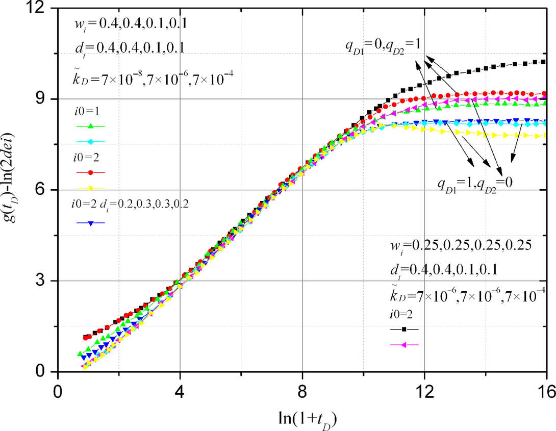
4.2.4 Behavior of Function g − ln(2dei)
Fig. 4.12 shows the change of ![]() with time for different four-layer reservoirs when
with time for different four-layer reservoirs when ![]() . It can be seen from the figure that
. It can be seen from the figure that ![]() are parallel straight lines, very near to each other in the first straight line period. In Chapter 2, it has been shown that for different two-layer reservoirs, functions
are parallel straight lines, very near to each other in the first straight line period. In Chapter 2, it has been shown that for different two-layer reservoirs, functions ![]() become a single straight line in the first straight line period. In Fig. 4.12, these parallel lines, quite near to each other, indicate that the two sections behave much like two large layers and
become a single straight line in the first straight line period. In Fig. 4.12, these parallel lines, quite near to each other, indicate that the two sections behave much like two large layers and ![]() ,
, ![]() , de1, and de2, defined by Chapter 3, can serve as productivities and diffusivities of the two large layers.
, de1, and de2, defined by Chapter 3, can serve as productivities and diffusivities of the two large layers.
 with time for different four-layer reservoirs and different producing section i (i=1 or 2). (After Gao (1983b) SPE 12580, Permission to publish by the SPE, Copyright SPE.)
In Chapter 2, we have seen that for a two-layer reservoir ![]() is a curve with one peak, and the peak value is approximately ln (d1/d2). d1/d2 can be determined approximately by the peak value of the above curve. d1 and d2 can be obtained by using
is a curve with one peak, and the peak value is approximately ln (d1/d2). d1/d2 can be determined approximately by the peak value of the above curve. d1 and d2 can be obtained by using ![]() .
.
Since the productivities and diffusivities of the two sections have been defined in this chapter, and Fig. 4.12 was shown to be reasonable, we can treat the present problem similar to the two-layer case. Using the simulation results for different four-layer reservoirs, the curves of ![]() versus time are shown in Figs. 4.13 and 4.14. The corresponding values of ln (de1/de2) are also shown in the figures. It can be seen from the figures that, similar to the two-layer case, the peak value here is approximate to ln (de1/de2) if
versus time are shown in Figs. 4.13 and 4.14. The corresponding values of ln (de1/de2) are also shown in the figures. It can be seen from the figures that, similar to the two-layer case, the peak value here is approximate to ln (de1/de2) if ![]() is not large. The semipermeability changes within sections do not influence the peak value of the curve; they only influence the tail trend of the curves. Therefore, we still can use the peak value of
is not large. The semipermeability changes within sections do not influence the peak value of the curve; they only influence the tail trend of the curves. Therefore, we still can use the peak value of ![]() as a rough estimation of ln (de1/de2).
as a rough estimation of ln (de1/de2).
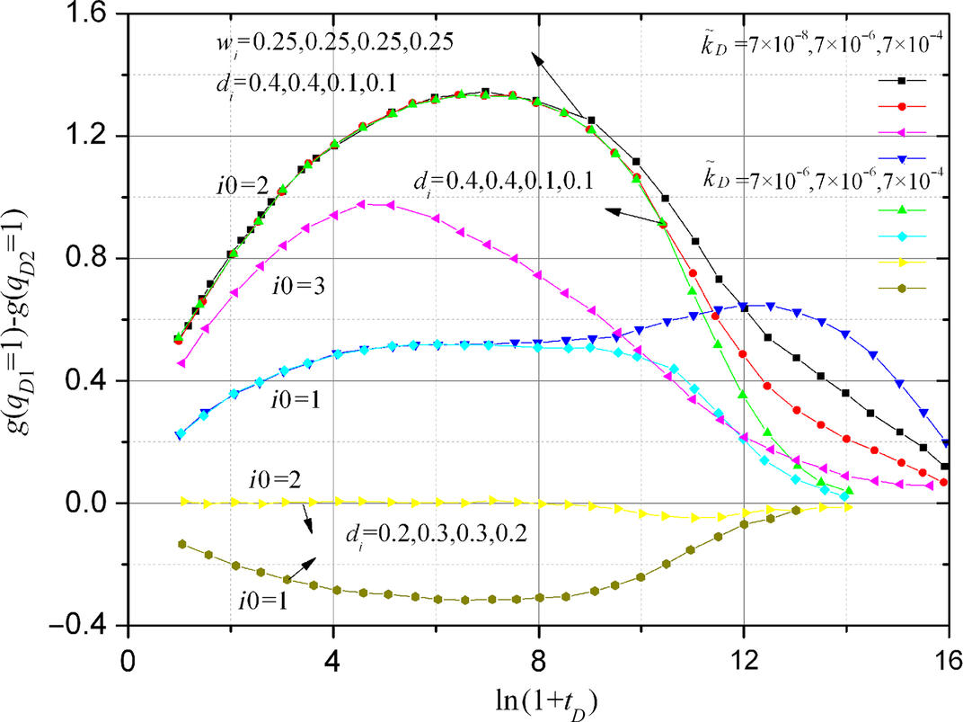
 with time for different four-layer reservoirs. (After Gao (1983b) SPE 12580, Permission to publish by the SPE, Copyright SPE.)
 with time for different four-layer reservoirs. (After Gao (1983b) SPE 12580, Permission to publish by the SPE, Copyright SPE.)
From Figs. 4.13 to 4.14 it still can be seen that the peak value can be larger or smaller than ln (de1/de2). This shows the approximate nature of treating the two sections as two layers.
The approximate method for calculating di is as follows: determine the peak values of curves ![]() versus time from the well test data for
versus time from the well test data for ![]() . The peak values can be used as a approximation of ln (de1/de2). We get
. The peak values can be used as a approximation of ln (de1/de2). We get ![]() equations for di. Using relation
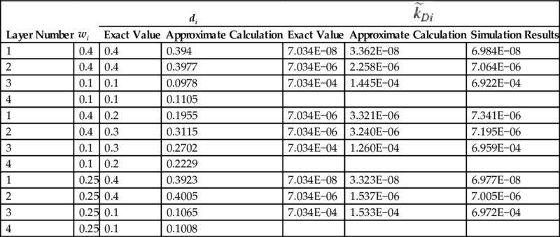
equations for di. Using relation ![]() and definition Eq. (4.12) for de1 and de1, the approximate values of d1,d2,…,dn, can be obtained. The calculation results for some four-layer reservoirs, using this method, are shown in Table 4.1. From Table 4.1 it can be seen that this simple method can give a useful value of di in most cases.
and definition Eq. (4.12) for de1 and de1, the approximate values of d1,d2,…,dn, can be obtained. The calculation results for some four-layer reservoirs, using this method, are shown in Table 4.1. From Table 4.1 it can be seen that this simple method can give a useful value of di in most cases.
Table 4.1
Comparison of Results
| Layer Number | wi | di | ||||
| Exact Value | Approximate Calculation | Exact Value | Approximate Calculation | Simulation Results | ||
| 1 | 0.4 | 0.4 | 0.394 | 7.034E−08 | 3.362E−08 | 6.984E−08 |
| 2 | 0.4 | 0.4 | 0.3977 | 7.034E−06 | 2.258E−06 | 7.064E−06 |
| 3 | 0.1 | 0.1 | 0.0978 | 7.034E−04 | 1.445E−04 | 6.922E−04 |
| 4 | 0.1 | 0.1 | 0.1105 | |||
| 1 | 0.4 | 0.2 | 0.1955 | 7.034E−06 | 3.321E−06 | 7.341E−06 |
| 2 | 0.4 | 0.3 | 0.3115 | 7.034E−06 | 3.240E−06 | 7.195E−06 |
| 3 | 0.1 | 0.3 | 0.2702 | 7.034E−04 | 1.260E−04 | 6.959E−04 |
| 4 | 0.1 | 0.2 | 0.2229 | |||
| 1 | 0.25 | 0.4 | 0.3923 | 7.034E−08 | 3.323E−08 | 6.977E−08 |
| 2 | 0.25 | 0.4 | 0.4005 | 7.034E−06 | 1.537E−06 | 7.005E−06 |
| 3 | 0.25 | 0.1 | 0.1065 | 7.034E−04 | 1.533E−04 | 6.972E−04 |
| 4 | 0.25 | 0.1 | 0.1008 | |||
Using the formula given in Chapter 2 for the two-layer case, we get the following formula for calculating the steady value of ![]() , denoted by
, denoted by ![]() , for the two-section case:
, for the two-section case:
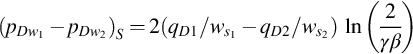
where ![]() and
and
From Eqs. (4.17), (4.18), we can get
where
The calculation results for some four-layer reservoirs, using formula Eq. (4.19), are given in Table 4.1. The values gS, needed in Eq. (4.19), are obtained by simulating the drawdown test for ![]() on the computer.
on the computer.
From Table 4.1 it can be seen that the semipermeabilities calculated by this approximate method have the correct order of magnitude, but they are smaller than the correct values. This can be explained: when we treat the two sections as two layers, it is equivalent to setting the semipermeabilities within the sections to be infinite and adding their resistance to the semipermeable wall between the two sections. Thus, the calculated semipermeability between the two sections is always smaller than it should be. It is easy to understand when the semipermeability between the sections is much smaller than that within the sections, this approximate method can give good results. When the semipermeability between sections is larger than that within the sections the added resistance might influence the semipermeability greatly. That is why the calculation results are not good when the semipermeability between sections is large. However, in practice, the approximate method still can give useful semipermeabilities.
For a more accurate evaluation of semipermeabilities, the simulation method can be used. A software has been developed that can accurately calculate the semipermeabilities ![]() of a multilayer reservoir even if each layer has a skin factor. When the software is used to calculate semipermeabilities, the productivities wi, the diffusivities di, and the steady values
of a multilayer reservoir even if each layer has a skin factor. When the software is used to calculate semipermeabilities, the productivities wi, the diffusivities di, and the steady values ![]() for
for ![]() need to be input as known parameters. The semipermeabilities, obtained by the simulation method for some four-layer reservoirs, are also listed in Table 4.1. It can be seen from the table that the simulation method gives very accurate semipermeabilities. The computer time needed is very short. For example, the calculation requires only two minutes of CPU time for a four-layer reservoir simulation.
need to be input as known parameters. The semipermeabilities, obtained by the simulation method for some four-layer reservoirs, are also listed in Table 4.1. It can be seen from the table that the simulation method gives very accurate semipermeabilities. The computer time needed is very short. For example, the calculation requires only two minutes of CPU time for a four-layer reservoir simulation.
4.3 New Drawdown Test
For the purpose of obtaining wi, and ![]() , a series of new drawdown tests need to be completed in a well.
, a series of new drawdown tests need to be completed in a well.
From Figs. 4.2 to 4.4 it is clear that the steady value ![]() will not change with di. Any rough estimation of di can be used in the simulation and it will not influence the accuracy of the semipermeabilities obtained. The productivity wi and
will not change with di. Any rough estimation of di can be used in the simulation and it will not influence the accuracy of the semipermeabilities obtained. The productivity wi and ![]() are the parameters we will obtain from the following new drawdown tests.
are the parameters we will obtain from the following new drawdown tests.
In an n-layer reservoir, all the layers are perforated. Layers 1 to i0 are perforated and produce with a fixed total rate and have a common wellbore pressure ![]() . Layers
. Layers ![]() to n are closed
to n are closed ![]() and have a common wellbore pressure
and have a common wellbore pressure ![]() . Because of crossflow,
. Because of crossflow, ![]() will change with time. Both
will change with time. Both ![]() and
and ![]() are measured in the test period. Generally, the
are measured in the test period. Generally, the ![]() versus log t curve consists of two straight lines with a transition period between them. The test must continue until the second straight line begins to appear. Set
versus log t curve consists of two straight lines with a transition period between them. The test must continue until the second straight line begins to appear. Set ![]() and repeat the test. In the second straight line period,
and repeat the test. In the second straight line period, ![]() and
and ![]() will change at the same rate with time.
will change at the same rate with time. ![]() will become a constant value
will become a constant value ![]() . The slope mi0 of the first straight line is equal to
. The slope mi0 of the first straight line is equal to  , so from
we can determine the productivity wi. Using these data we can calculate semipermeabilities by the simple calculation method or the simulation method.
4.4 Summary
The following conclusions can be obtained:
(1) In a multilayer reservoir, the distributions of pressures in two neighboring layers are mainly the same in the region far from the well if the semipermeability between the two layers is large.
(2) When the crossflow caused by different boundary pressures exists in the vicinity of the well in one layer, there will be crossflow induced in the other layers in the vicinity of the well, no matter if the layers have the same wellbore pressure as their neighboring layers or not. The crossflow near the boundaries will increase with time at first and gradually approach a steady state.
(3) The crossflow, caused only by different diffusivities between layers, can be described approximately by Eq. (4.13). With an increase in time, the peak point will travel way from the well. This kind of crossflow is determined only by the equations and the total production rate at the well, and it does not depend on which layers or how many layers produce.
(4) The new drawdown test can be used to evaluate semipermeabilities between layers.