
Material Balance Equation of Multilayer Gas Reservoir
Abstract
In recent years, more and more multilayer gas reservoirs have been discovered worldwide. Dynamic reserve estimation of multilayer producers is a major challenge for reservoir engineering. The material balance equation (p/Z plot) is one of the fundamental methods for reserve estimation. It is usually used in single-layer gas reservoir.
In Section 10.1, we study the applicability of the multilayer gas reservoir material balance equation for reserve estimation by single well numerical simulation. There are several parameters that are implicated in the reserve estimation of multilayer gas reservoirs, such as the connectivity between layers of the gas reservoir, the difference between formation pressures of the layers, and the difference between permeability of the layers.
In Section 10.2, we present a new method to estimate the single well dynamic reserve and individual reserve recovery for two-layer commingled gas reservoirs, which provides a foundation for the reasonable and efficient development of multilayered gas reservoir.
In Section 10.3, we establish a material balance equation of gas reservoir with a supplying region and performance forecast method by the semipermeable wall model. The results on real cases indicate that the proposed model can improve the accuracy of early performance forecast.
Keywords
Multilayer gas reservoir; Material balance equation; Dynamic reserve; Supplying region; Performance forecast; Semipermeable wall model
10.1 Material Balance of Two-Layer Gas Reservoir
The dynamic reserve estimation is one of the major tasks in gas field development. The dynamic reserve is the produced original gas in place (OGIP) that is estimated with a dynamic method when formation pressure reduces to zero. Calculation methods include the material balance method (Sun, 2011a), elastic binomial, extended drawdown test, production decline analysis method, numerical simulation, etc.
The material balance method is the main method for reserve estimation in a gas field. One of the basic assumptions of the method is that a gas reservoir consists of a single and homogeneous gas tank. The recovery percent of reserve should be higher than 5% as the method applies to reserve estimation. Several successful analyses have been performed on single-layer reservoirs. However, the classic material balance equation is unable to accurately forecast production performance of the multilayer gas reservoir.
The multilayer gas reservoir can be divided into two types depending on the existence of crossflow between layers. It is a commingled system if the layers have been isolated by a nonpermeable layer, while it is a crossflow system if there is connectivity between layers.
The production performances of multilayer reservoirs with or without crossflow are different. For a multilayer reservoir without crossflow, the individual layer rate is proportional to the formation flow capacity (kh) when the skin factor is the same for all the layers in the early period; the individual layer rate is proportional to the individual layer reserve in the long time period (PSSF).
For a multilayer reservoir with crossflow, flow is more complicated. For a circled closed multilayer reservoir with crossflow, the individual layer rate is relevant to skin factor, formation flow capacity (kh), and communication between zones. When the skin factors are the same, the individual layer rate is proportional to the formation flow capacity (kh); when the skin factors are different, the smaller the skin factor, the larger the individual layer rate is.
10.1.1 Physical Model
Assuming the gas reservoir is divided into two interconnected relatively homogeneous blocks, as shown in Fig. 10.1, we can concentrate the plane flow resistance to the flow at the wall between the blocks and assume the flow resistance is zero within the block. Under this scenario, the pressure within the block is only time-related. Semipermeable wall resistance on the flow can be calculated by the equivalent flow resistance method, as shown in Eq. (10.1). The semipermeable wall model can be used any time to ensure that the pressure is balanced within the block, so each district can meet the conditions of traditional material balance. In this model, the heterogeneity and the flow resistance of the stratum are considered, which makes the material balance much closer to the practical cases.


The following assumptions are used in this section. The multilayer reservoir is homogeneous, isotropic, horizontal, and infinite. There are homogeneous, low permeability, and thin shales between layers; the storage of the shale is negligible compared to that of the layers. The reservoir is filled with a slightly compressible fluid of small and constant compressibility, and the flow obeys Darcy's law; the gravity can be neglected; a well completely penetrates the reservoir; the skin of the well is infinitely thin; and the well produces with a constant rate q from t=0. The multilayer reservoir is modeled by the semipermeable model.
10.1.2 Mathematical Model of a Two-Layer Gas Reservoir Without Crossflow
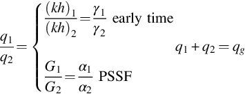
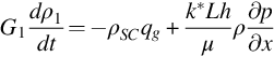
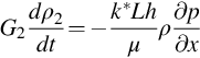
The material balance for gas is described by the following pair of equations:
and
For a multilayer reservoir without crossflow, the individual layer rate is
The individual layer pressure is

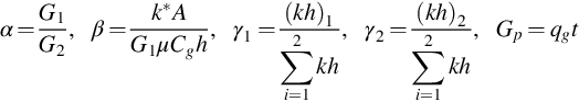
where
10.1.3 Mathematical Model of a Two-Layer Gas Reservoir with Crossflow
The material balance for gas is described by the following pair of equations:


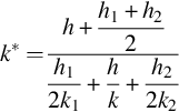
For a multilayer reservoir with crossflow, the individual layer rate is

where k* is average permeability:
Initial condition:
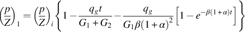
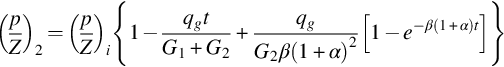
The individual layer pressure is

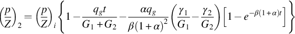
where
10.1.4 p/Z Curve of a Two-Layer Gas Reservoir
10.1.4.1 p/Z Curve of a Two-Layer Gas Reservoir Without Crossflow
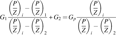
There are two lines for a p/Z curve of a two-layer gas reservoir without crossflow. The slopes are ![]() and
and ![]() respectively. The OGIP is
respectively. The OGIP is ![]() when
when ![]() , as shown in Fig. 10.2.
, as shown in Fig. 10.2.
10.1.4.2 p/Z Curve of a Two-Layer Gas Reservoir with Crossflow
Early Time Period
In the early time, ![]() , the derivatives of Eqs. (10.12), (10.13) are
, the derivatives of Eqs. (10.12), (10.13) are
In the early time, the slope is identical to the case where there is no crossflow. The pressure difference of the two layers is so small that the crossflow rate can be neglected.
Long Time Period
In the PSSF, ![]() , the derivatives of Eqs. (10.12), (10.13) are
, the derivatives of Eqs. (10.12), (10.13) are
There are also two lines for the p/Z curve of a two-layer gas reservoir with crossflow. The OGIP is ![]() when
when ![]() , as shown in Fig. 10.3. In the long time, OGIP is
, as shown in Fig. 10.3. In the long time, OGIP is ![]() as a single layer.
as a single layer.
10.1.5 Influencing Factor Analysis of Reserve Estimation
Parameters used in simulation are as follows: the well is drilled with two zones, the supply radius is 750 m, and the vertical permeability is the same for the two zones. The wellbore diameter is 0.1 m, the thickness is 20 m, and permeability is 0.1 md for each zone; the formation temperature is 80 °C, original formation pressure is 20 MPa, relative density of natural gas is 0.6, pseudocritical pressure is 4.67 MPa, and pseudocritical temperature is 195.7 K. Suppose a single well is put into production with an output of 5×10⁴ m3/d, the production cycle is 300 d, and the time of shut-in is 30 d. Six cycles are simulated and accumulative gas production is 0.9×10⁸ m3. The highest shut-in pressure is used for the average formation pressure for reserve estimation.
10.1.5.1 The Effect of an Interlayer Heterogeneity on Dynamic Reserve Estimation
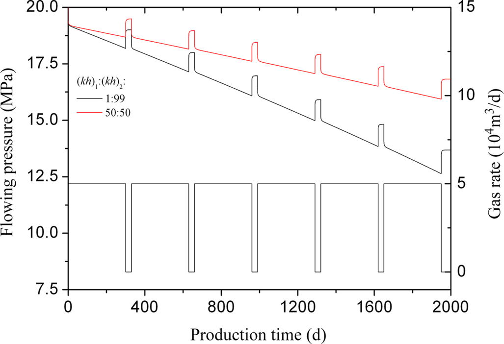
The following assumptions are made: the two zones have the same thickness of 10 m and the sum of the permeability-thickness product is 100 md.m. Dynamic reserve estimation on different permeability-thickness product is shown in the Fig. 10.4. The result of the dynamic reserve decreases with the increased heterogeneity between layers. When the permeability-thickness product of the two zones is 1:99, the reserve estimation is 2.85×10⁸ m3, which is 48.5% of the reserve (5.88×10⁸ m3)when the permeability-thickness product of the two zones is equal to each other.
The average formation pressure is determined by the shut-in pressure buildup. The measured average pressure by this way is not to represent the average pressure of the multilayer formation, but it is closer to the average pressure of the weak zone. The simulation result indicated that the more heterogeneity the layer is, the more the pressure declines, and the lower the measured formation pressure is, as shown in Fig. 10.5. Therefore, if the apparent formation pressure, p/Z, is less than expected, the reserve estimation would be lower.
10.1.5.2 The Effect of Crossflow on Dynamic Reserve Estimation
If there is crossflow between two adjacent zones, the flow could be considered as linear flow. On the basis of the linear flow equation of Darcy's law, the interlayer crossflow could be calculated by the following formula:

where the flow distance is half of the thickness of two adjacent formations:
The vertical permeability of the two adjacent zones is

Assuming that the total of permeability-thickness product of the two zones is 100 md.m, the simulation result indicates that the vertical permeability has a great impact on the reserve estimation, as shown in Fig. 10.6.
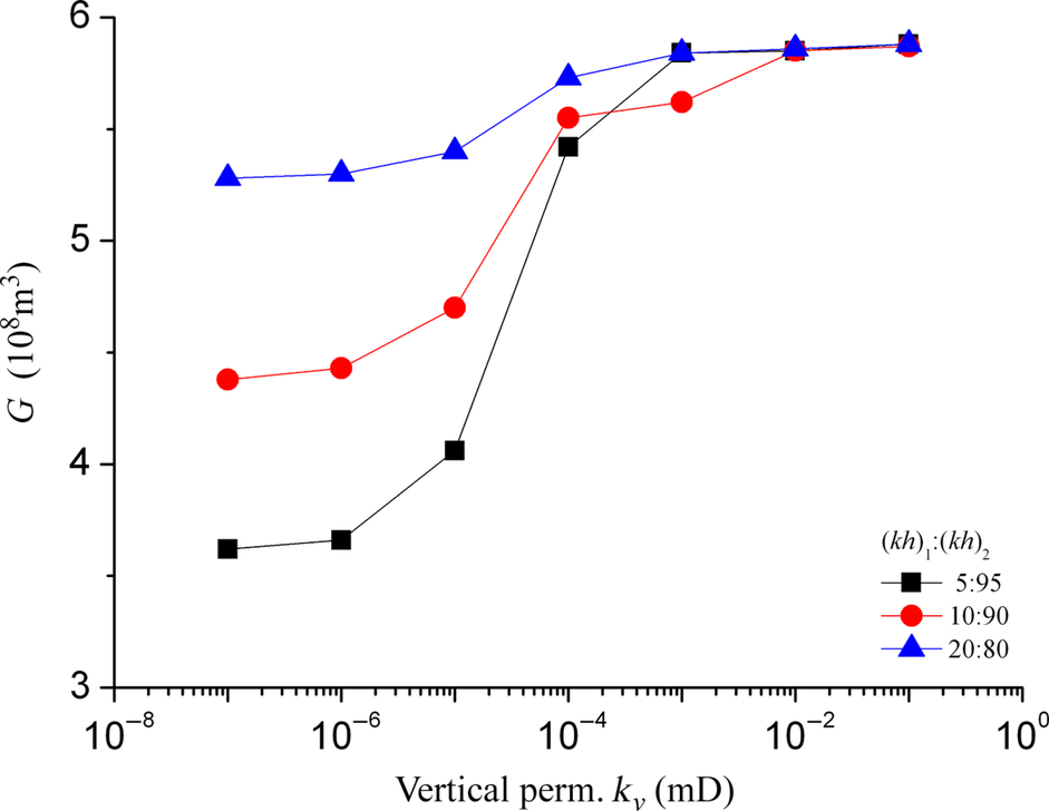
When the vertical permeability is smaller than 1E−4 md, the more heterogeneity is, the less dynamic reserve declines are. When the permeability is 1:4, the reserve estimation is nearly 90% of the OGIP although the vertical permeability is only 1E−7 md. However, when the permeability is 1:19, the reserve estimation is only 60% of the OGIP.
When the vertical permeability value exceeds 1E−4 md, the heterogeneity has little impact on the reserve estimation and the dynamic reserve is close to 5.88×10⁸ m3.
The above results indicate that the crossflow between the two zones is under the control of interzonal permeability. Although the vertical permeability is a small value, the exchange volume in the whole contact area is large. When the vertical permeability is above 1E−4 md, it plays an important role in interzonal pressure balance.
10.1.5.3 The Effect of the Permeability on Reserve Estimation
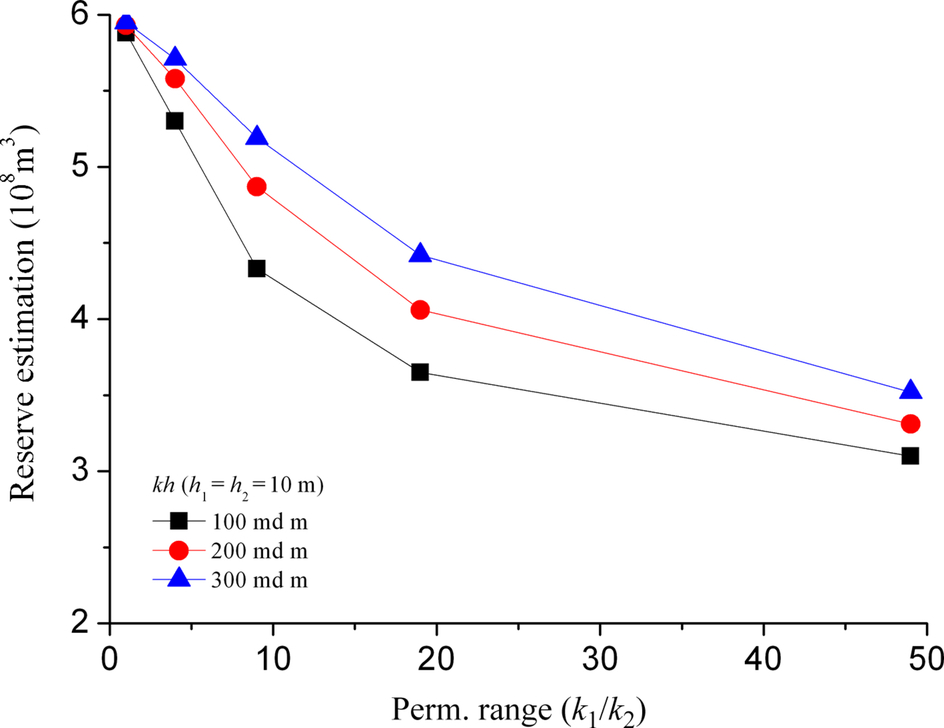
Suppose that the permeability-thickness products are 100, 200, and 300 md.m respectively and the thickness of each zone is 10 m. Dynamic reserve estimation under different permeability is shown in Fig. 10.7. The permeability and permeability-thickness product both influence the reserve estimation. With the same permeability-thickness product, the higher the permeability value, the larger the reserve estimation is.
10.1.6 Method of Improving the Ratio of Dynamic Reserve to OGIP
10.1.6.1 Well Stimulation for Formation with Low Permeability
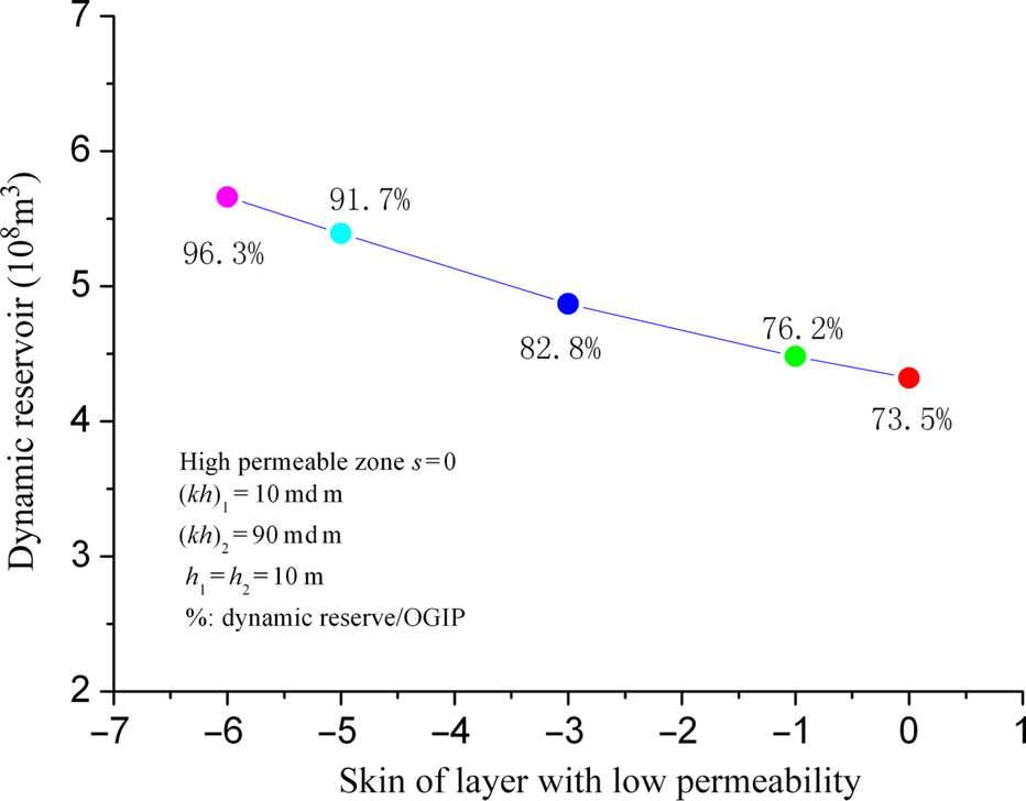
Suppose that the permeability-thickness products are 10 and 90 md.m, respectively, the thickness of each zone is 10 m, and the skin factor of the high permeable zone was 0. Dynamic reserve estimation under different skin factors is shown in Fig. 10.8. If the skin factor of each zone is zero, the ratio of dynamic reserve to OGIP is only 73.5%. If the layer with low permeability is stimulated and when the skin factor is less than −5, the ratio of dynamic reserve to OGIP is above 91.7%.
10.1.6.2 Reduce the Production Output
Suppose that the permeability-thickness products are 10 and 90 md.m respectively, the thickness of each zone is 10 m, and the skin coefficient is zero for each zone. Firstly, the production is implemented with an output of 5×10⁴ m3/d, and an adjustment is made at a later stage. The dynamic reserve estimation result is shown in Fig. 10.9. If the skin factor of each zone is zero, the ratio of dynamic reserve to OGIP is only 73.5%. If a certain adjustment of production output is made at a later stage of development, the producing reserve could be improved. When the production output is adjusted at 3×10⁴ m3/d, the ratio of dynamic reserve to OGIP would be as high as 84.5%.

10.1.6.3 Single-Layer Production for Layer with Low Permeability
The interlayer replacement could be adopted and layer with low permeability may produce independently to improve the accuracy of dynamic reserve.
10.2 Reserve Estimation of a Two-Layer Commingled Gas Well
Multilayer reservoirs can be divided into two types according to the crossflow between layers, that is, crossflow reservoirs and no-crossflow (commingled) reservoirs. The commingled production is an effective way to develop the multilayer gas reservoir without crossflow. Performance of commingling wells are different due to the differences in average pressures, the permeabilities, and OGIP.
10.2.1 Physical Model and Mathematical Model
Assume the gas reservoir consists of two layers, there is no interlayer fluid exchange, and each layer is in line with the traditional material balance conditions, as shown in Fig. 10.10. In addition, (1) the reserves of the layers are G1, G2 respectively, and the reserve in barrier is ignored; (2) the single well production is q (the layer productions are q1, q2, respectively); (3) the single well cumulative production is Gp (the layer cumulative productions are Gp1, Gp2 respectively); (4) the water effect is negligible; and (5) the initial formation pressure is the same.

The layered material balance equation is


According to Eqs. (10.18)–(10.20) can be derived as
Assume
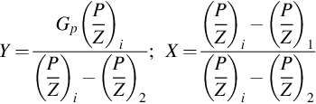
Then
It can be seen that, X~Y is a linear relationship. Thus, the individual reserve parameters can be obtained by the measured point's data regression, and the individual recovery percent of reserve can be established. This calculation requires at least two shut-in pressure calculations with one run-in-hole.
10.2.2 Examples
Well parameters are as follows. Two layers are drilled, and the supply radius is about 1000 m. The wellbore radius is 0.1 m, and the total thickness of formation is 20 m; the porosity of each layer is equal to 0.1, the formation temperature is 80 °C, the initial formation pressure is 30 MPa, the natural gas relative density is 0.6, the pseudocritical pressure is 4.67 MPa, and the pseudocritical temperature is 195.7 K. The OGIP is 7.65×10⁸ m3, respectively; permeability-thickness product of the first layer, (kh)1, is about 30 md.m, and permeability-thickness product of the second layer, (kh)2, is about 10 md.m. The well produces for 2500 d at a 10 MPa constant bottomhole flowing pressure. Cumulative gas production of the first layer is 3.80×10⁸ m3, and the cumulative gas production of the second layer is 1.9×10⁸ m3.
Fig. 10.11 is a data match curve in Table 10.2. The individual dynamic reserves are 7.72×10⁸ and 7.62×10⁸ m3 respectively, for which the errors compared with the original reserves are 0.9% and 0.4% respectively, and the error compared with OGIP is 0.26%.

Table 10.1
Two-Layer Gas Reservoir Stimulation Results at a Constant Pressure
| Production Time (d) | Total Production (104 m3) | First Layer | Second Layer | ||
| p/Z (MPa) | GP1 (104 m3) | p/Z (MPa) | GP2 (104 m3) | ||
| 0 | 0 | 30.83 | 0 | 30.83 | 0 |
| 10 | 509 | 30.68 | 374 | 30.78 | 135 |
| 20 | 912 | 30.56 | 671 | 30.73 | 241 |
| 30 | 1340 | 30.43 | 985 | 30.69 | 355 |
| 40 | 1765 | 30.31 | 1297 | 30.64 | 468 |
| 50 | 2188 | 30.18 | 1607 | 30.60 | 581 |
| 60 | 2609 | 30.06 | 1915 | 30.55 | 694 |
| 70 | 3027 | 29.93 | 2221 | 30.50 | 806 |
| 80 | 3442 | 29.81 | 2524 | 30.46 | 918 |
| 90 | 3855 | 29.69 | 2826 | 30.42 | 1029 |
| 100 | 4265 | 29.57 | 3125 | 30.37 | 1140 |
| 200 | 8232 | 28.41 | 6005 | 29.93 | 2227 |
| 300 | 11,960 | 27.33 | 8684 | 29.51 | 3276 |
| 400 | 15,461 | 26.33 | 11,174 | 29.10 | 4287 |
| 500 | 18,746 | 25.40 | 13,484 | 28.71 | 5262 |
| 1000 | 32,344 | 21.68 | 22,709 | 26.95 | 9635 |
| 1500 | 42,282 | 19.14 | 29,006 | 25.48 | 13,276 |
| 2000 | 50,000 | 17.26 | 33,671 | 24.25 | 16,329 |
| 2500 | 56,939 | 15.52 | 38,000 | 23.20 | 18,939 |
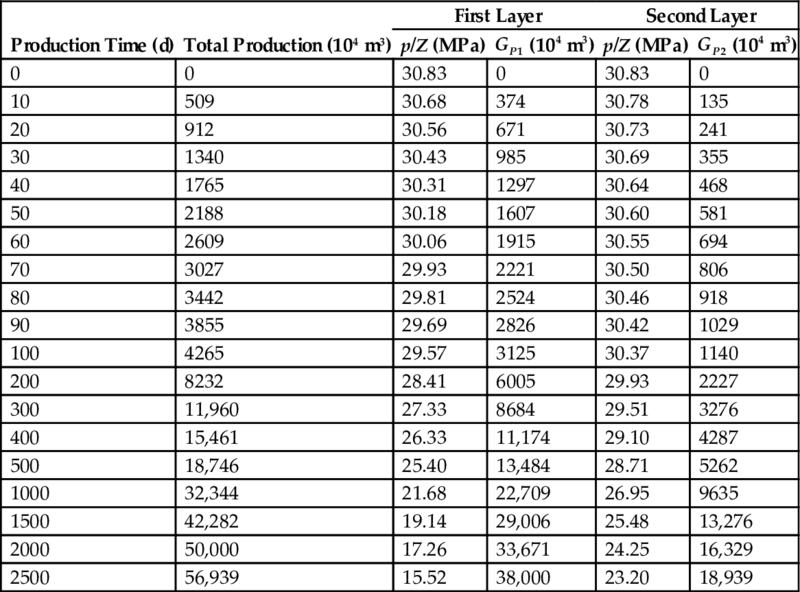
Table 10.2
Two-Layer Gas Reservoir Dynamic Reserve Calculation (Adjacent Point)
| Production Time (d) | Total Production (104 m3) | Y (108 m3) | X | GP1 (108 m3) | GP2 (108 m3) | GP1 Error (%) | GP2 Error (%) | G Error (%) |
| 0 | 0 | 0 | 0 | |||||
| 10 | 509 | 28.7810 | 2.7713 | |||||
| 20 | 912 | 28.8220 | 2.7726 | 30.388 | 55.434 | |||
| 30 | 1340 | 28.8165 | 2.7703 | 2.341 | 22.330 | 69.4 | −191.9 | −61.2 |
| 40 | 1765 | 28.7964 | 2.7668 | 5.802 | 12.742 | 24.2 | −66.6 | −21.2 |
| 50 | 2188 | 28.7703 | 2.7629 | 6.657 | 10.379 | 13.0 | −35.7 | −11.3 |
| 60 | 2609 | 28.7412 | 2.7588 | 7.019 | 9.378 | 8.3 | −22.6 | −7.2 |
| 70 | 3027 | 28.7103 | 2.7545 | 7.210 | 8.850 | 5.7 | −15.7 | −5.0 |
| 80 | 3442 | 28.6783 | 2.7501 | 7.325 | 8.534 | 4.3 | −11.6 | −3.7 |
| 90 | 3855 | 28.6456 | 2.7457 | 7.399 | 8.330 | 3.3 | −8.9 | −2.8 |
| 100 | 4265 | 28.6124 | 2.7412 | 7.450 | 8.189 | 2.6 | −7.0 | −2.2 |
| 200 | 8232 | 28.2708 | 2.6960 | 7.561 | 7.886 | 1.2 | −3.1 | −1.0 |
| 300 | 11,960 | 27.9270 | 2.6509 | 7.620 | 7.727 | 0.4 | −1.0 | −0.3 |
| 400 | 15,461 | 27.5865 | 2.6063 | 7.635 | 7.688 | 0.2 | −0.5 | −0.1 |
| 500 | 18,746 | 27.2510 | 2.5624 | 7.641 | 7.672 | 0.1 | −0.3 | −0.1 |
| 1000 | 32,344 | 25.6792 | 2.3569 | 7.646 | 7.658 | 0.1 | −0.1 | 0.0 |
| 1500 | 42,282 | 24.3630 | 2.1848 | 7.649 | 7.653 | 0.0 | 0.0 | 0.0 |
| 2000 | 50,000 | 23.4236 | 2.0620 | 7.649 | 7.652 | 0.0 | 0.0 | 0.0 |
| 2500 | 56,939 | 22.9990 | 2.0064 | 7.649 | 7.652 | 0.0 | 0.0 | 0.0 |
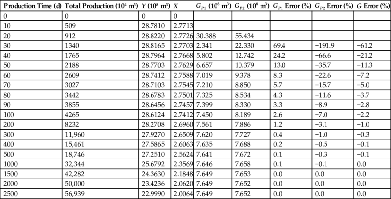
It can be seen from Table 10.2 that the individual reserve is calculated with two adjacent points: G1 is smaller than the theoretical values and G2 is larger than the theoretical values. In order to ensure that the error of dynamic reserves is <5.0%, the recovery percent of reserve must be >2.5%; in order to ensure that the error of the individual reserve is <5.0%, the recovery percent of reserve must be >5.0%.
10.3 Material Balance Equation of Gas Reservoir with a Supplying Region
The traditional method of material balance takes the gas reservoir as containers while the heterogeneity and the flow resistance of the stratum are neglected. Therefore, the results tend to be optimistic when using laminar-inertial turbulent flow analysis and the material balance equation to predict performance on heterogeneous gas reservoirs with low permeability. To improve the accuracy of performance forecast, a semipermeable wall model is proposed. According to the law of conservation of mass, a gas material balance equation with a supplying region and performance forecast method are established. Assuming the gas reservoir with low permeability is divided into two interconnected strips that are relatively homogeneous blocks, we can concentrate the plane flow resistance to flow at the wall between the blocks and let the flow resistance be zero within block. Hence, the pressure within the block is only time-related. Semipermeable wall resistance on the flow can be calculated by the equivalent flow resistance method. The semipermeable wall model can be used any time to ensure that the pressure balances within the block, so each district can meet the conditions of traditional material balance. In this model, the heterogeneity and the flow resistance of the stratum are considered, which makes the material balance much closer to the practical cases. In addition, the performance of well can be easily and simply forecast. The changing rules of pressure-time and rate-time are explained. The results on real cases indicate that the proposed model can improve the accuracy of the early performance forecast. This study can direct the rational and effective development of the similar gas reservoirs.
10.3.1 Introduction
Gas reservoir production performance forecast is the core task of gas field development management throughout the lifecycle of gas field development. In the beginning stages of the development of the gas field, the material balance method and the numerical simulation method were the main methods for performance forecast. The traditional material balance method is very simple. That is, the gas field is assumed as a homogeneous container, and gas reservoir heterogeneity is ignored completely. The result of forecasting always has a tendency for optimism. On the contrary, numerical simulation is too complex to be applied in general gas reservoir engineering. It requires the detailed formation parameter distribution, which is difficult to obtain in the early period of gas field development. Its application is limited when a large amount of work is required.
It is urgent to develop a method for gas reservoir production performance forecast in the early time of gas field development, which not only considers the regional heterogeneity, but also forecast the gas field performance quickly and easily. In recent years, the multitank material balance method is studied by several studies. Its result is reliable compared with the numerical simulation.
10.3.2 Material Balance Equation of Gas Reservoir with a Supplying Region
10.3.2.1 Physical Model
Assume the gas reservoir is divided into two interconnected relatively homogeneous blocks, as shown in Fig. 10.12. We can concentrate the plane flow resistance to flow at the wall between the blocks and let the flow resistance be zero within the block. Hence, the pressure within the block is only time-related. Semipermeable wall resistance on the flow can be calculated by the equivalent flow resistance method, as shown in Eq. (10.23). The semipermeable wall model can be used any time to ensure that the pressure balances within the block, so each district can meet the conditions of traditional material balance. In this model, the heterogeneity and the flow resistance of the stratum are considered, which makes the material balance much closer to the practical cases.


10.3.2.2 Mathematical Model
In the near-wellbore tank region, the material balance is
In the outer tank region, the material balance is
where k* is average permeability of the flow control region

The initial condition is
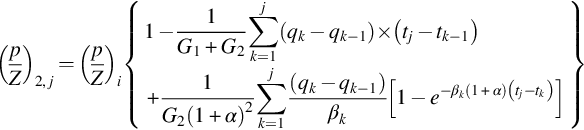
Individual region pressure is
where

For variable flow rate, according to Duhamel's principle, we have

10.3.2.3 Deliverability Equation and Recharge Equation
There is only one production well in the reservoir, and the deliverability equation is as follows:
The recharge flow rate is proportional to the pressure difference in two regions:

We can forecast the gas reservoir production performance by Eqs. (10.28)–(10.31).
10.3.3 Example and Discussion
10.3.3.1 Example
Parameters used in the example are as follows. The thickness is 10 m, as shown in Fig. 10.13. The near-wellbore tank region permeability is 10 md, the outer tank region permeability is 5 md, the low-permeability region permeability is 0.1 md, the absolute open flow potential is 59×104 m3/d, the formation temperature is 80 °C, the original formation pressure is 30 MPa, and the relative density of natural gas is 0.6. The deliverability equation is

10.3.3.2 p/Z Curve
The well is producing at a constant rate of 10.0×10⁴ m3; the relationship of the apparent formation pressure of the near-wellbore tank region and the produced gas volume is shown in Fig. 10.14. There is an obvious breakpoint.

In the early stages of well development, the pressure difference between the regions is very small, so the recharge rate can be neglected. The relationship of (p/Z)1 and Gp is a line, and the slope is ![]() . The derivative of Eq. (10.28) can be written as
. The derivative of Eq. (10.28) can be written as
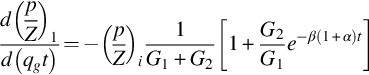
In the long time, the exponential term of Eq. (10.34) can be neglected, the second line appears, and the slope is ![]() , as shown in Fig. 10.13.
, as shown in Fig. 10.13.
The reserve derived from the multisection (p/Z)1 curve is lower than that of the conventional (p/Z) curve, and the reserve difference ΔG can be expressed as
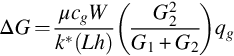
The above formula indicates that when the multiregion reserve keeps constant, ΔG depends on not only the characteristic parameters of the gas reservoir, but also the initial production associated with the production area. The residual reserve decreases with the increase of gas reservoir permeability and the contact area between the blocks. The residual reserve also decreases with the decrease of the stripe widths of the two intervals. The residual reserve increases with the increase of the production rate, which is consistent with the laboratory experiment result.
10.3.3.3 Performance Forecast
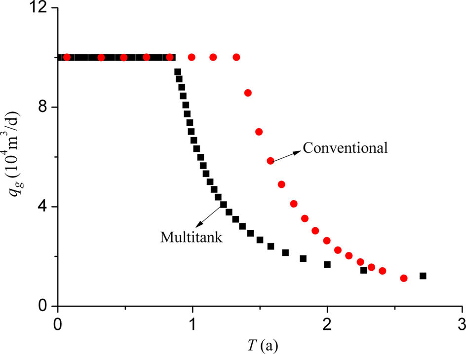
The well is producing at a constant rate of 10.0×10⁴ m3, and the result comparison of the conventional and multitank model is shown in Fig. 10.15. There is a difference about the period of stabilized production. It is 0.85a for the multitank model method and approximately 1.32a for the conventional method. The result of gas reservoir production performance forecast is shown in Fig. 10.16.

The numerical simulation method shows that the stable production period is 0.90 years if the well produces with a constant rate of 10.0×10⁴m3/d. The pressure field is shown in Fig. 10.17. The result of the multitank model is close to the result of the numerical simulation method.

10.4 Summary
(1) For a multilayer gas reservoir, if the individual thickness is the same for the two zones and there is no crossflow, the reserve estimation result is mainly influenced by interlayer heterogeneity and the permeability. Dynamic reserve declines as heterogeneity between layers increases. For the same permeability-thickness product of the formation, the higher the permeability is, the larger the individual reserve is.
(2) For a multilayer gas reservoir, if the individual thickness is the same for the two zones and there is crossflow, the reserve estimation result is mainly influenced by vertical permeability and heterogeneity between layers.
When vertical permeability is smaller than 1E−4 md and the permeability ratio of the two zones is above 1/4, the reserve estimation can be calculated by the material balance method. Moreover, the estimation error of the reserve is within 10%.
When vertical permeability is above 1E−4 md, the effect of heterogeneity on reserve estimation is little, and the estimation result is fairly accurate.
(3) The ratio of dynamic reserve to OGIP can be improved by means of well stimulation, optimization of production, replacement of different layers, etc.
(4) The recovery percent of the reserve can be analyzed by the layered material balance equation. The new calculation method is simple and practical; the individual reserve error is <5% when the recovery percent of the reserve is greater than 5.0%.
(5) For multiple wells with the same producing positions, the total gas reservoir shut-in approach should be applied to acquire the layer average formation pressure, and then the above method can be applied to estimate the dynamic reserve and evaluate the individual recovery percent of the reserve.
(6) For the case of more than two layers, firstly, all layers should be divided into two sets of layer groups according to geological knowledge; then the above method can be applied to estimate the dynamic reserve.
(7) The two-tank material balance model can be easily extended to the N-region model; it can be used to forecast the performance of gas reservoir with serious heterogeneity.
(8) The two-tank model is based on the condition that the deliverability equation is reliable. For low-permeability or tight gas reservoir, the deliverability equation is not reliable, so the result of forecast will make a great difference.