
Interpretation Theory for Vertical Interference Testing Across a Low-Permeability Zone
Abstract
An interpretation theory for the vertical interference testing across a low-permeability zone is given, which includes skin factor of each layer, wellbore storage, interlayer crossflow, leakage behind the casing, and storativity of the low-permeability zone. The inclusion of the storativity of the low-permeability zone makes the calculated pressures for both the active and the observation zones much closer to the measured pressures. The inclusion of the leakage behind the casing makes it possible to interpret the vertical interference test of a well that is poorly cemented. It also provides a tool for studying the leakage behind the casings.
Both the variable flow rate case and the constant surface rate case are studied. The reservoir parameters can be interpreted in the Laplace space as well as in real space. It is suggested to measure the wellbore pressures of both the active and observation zones when leakage behind the casing exists, which will make the interpretation easier and more reliable. The influence of various parameters on wellbore pressure and its derivative is studied through simulation results. The limiting behavior at short time and long time is studied for a constant surface rate. It shows that the leakage behind the casing and the pressure difference between the active and the observation layers will become steady when time is long enough. This steady pressure difference can determine the semipermeability.
Keywords
Vertical interference test; Multilayer reservoir; Multilayer well test; Interlayer crossflow; Leakage behind the casing
8.1 Introduction
In developing a suitable exploitation method for oil and gas reservoirs, knowledge of the vertical permeability of the reservoir is needed. This is particularly true for a thick reservoir or a layered reservoir undergoing secondary or tertiary recovery.
The vertical interference testing is a method for determining horizontal and vertical properties of a reservoir near the well by analyzing pressure transients opposite an isolated set of perforations while the well is flowed or pulsed at another depth. Vertical interference tests have been used to determine the vertical permeability in a single zone or in the low-permeability layer separating two productive zones, to determine crossflow between the two zones and to detect leakage behind the casing.
Methods for determination of vertical permeability in a single zone were provided by several authors (Burns, 1969; Prats, 1970; Falade and Brigham, 1974; Hirasaki, 1974; Earlougher, 1980; Kamal, 1986). Earlougher compared the various methods and considered wellbore storage at both the active and observation zones, leakage behind the casing, and vertical flow across a permeability barrier in the formation. Kamal provided a new type of curve set for the early time testing data. However, these methods are not suitable for stratified reservoirs with several layers having quite different properties.
In Chapters 2 and 7, we provided an interpretation method of the reservoir properties based on semilog straight line portions of both the active and observation pressures. We also presented a detailed discussion of the crossflow behavior between layers. Our method neglects the wellbore storage and uses the early time data to determine layer parameters. Several authors (Bremer et al., 1985; Ehlig-Economides and Ayoub, 1986; Lee et al., 1984; Wijesinghe and Kececioglu (1988) have studied the vertical interference test in a three-layered reservoir with the middle layer being a thin tight one. Bremer et al., (1985) presented a curve method for the observation pressure to estimate reservoir parameters. This method assumed identical formation properties except thickness for both the active and observation layers, and it neglected the skin factor and wellbore storage. Ehlig-Economides and Ayoub (1986) eliminated the above restrictions. They presented a detailed analysis of the asymptotic behavior of the pressure and used both the active and observation pressures in type curve matching. In the above studies, steady-state crossflow in the tight middle layer is assumed. Lee et al. (1984) presented an improved analysis for pulse tests, which assumed unsteady crossflow in the tight middle layer. Instead of using type curve matching, they used nonlinear parameter estimation. Wijesinghe and Kececioglu (1988) compared the behavior of the steady-state crossflow and the unsteady crossflow in the tight layer and showed their influence on active and observation pressures. They found that the pressures of the active layer for unsteady crossflow and steady-state crossflow are close to each other at an early time and are almost the same at a long time. But the observation pressure for unsteady crossflow is far different from that for steady-state crossflow in the early time, which is called the middle time period in Chapter 7. Therefore, the interpretation methods, which are based on the steady-state crossflow assumption and use the observation pressure in type curve matching or analysis, may provide the wrong results. The interpretation methods, which are based on the steady-state crossflow assumption and use only the pressure of the active layer in analysis, should still work.
Because of bad cementing or hydraulic fracturing, leakage behind the casing is found in many wells. Earlougher (1980) showed that a micro-annulus of only 25 μm (0.001 in.) wide will give enough vertical flow between observation and active perforations to cause the appearance of a high vertical permeability. He simulated the micro-annulus by adding a very large vertical permeability at the nodes close to the well in a program, but he did not give a detailed analysis. To the author's knowledge, this is the only treatment of the leakage behind the casing. Overall, the study of the transient testing on wells with leakage behind the casing is very poor and a theory is earnestly needed in practice. The objective of this chapter is to give a well testing theory to analyze and interpret the vertical interference test conducted at a three-layered reservoir, including skin factors, wellbore storage of the active layer, the compressibility of the low-permeability middle layer, and the fluid leakage behind the casing.
8.2 Model Description
Suppose a reservoir consists of two permeable layers, separated by a third layer of comparatively low permeability. A well drilled the reservoir completely. A packer is located at the low-permeability middle layer and separates the two productive layers, and a micro-annulus behind the casing allows communication of fluid between the two productive layers under the pressure difference between them.
Because the observation pressure may be used in the analysis, the compressibility of fluid in the low-permeability middle layer cannot be neglected (Gao, 1984; Bremer et al., 1985; Ehlig-Economides and Ayoub, 1986), but the horizontal flow in it can be neglected. Therefore, the following assumptions are used:
(1) A three-layered reservoir is infinite, homogeneous, isotropic, and filled with a single-phase fluid of slight compressibility and constant viscosity. The middle layer has low permeability.
(2) A well penetrates the reservoir completely. A packer is located at the middle layer and separates the upper and lower ones. Vertical communication may occur through the micro-annulus between the casing and the wall of the well or through the packer.
(3) The horizontal flow in the low-permeability middle layer is negligible.
(4) Flow obeys Darcy's law. The gravity force is neglected.
(5) The semipermeable wall mode is used in replace of the actual reservoir.
According to the semipermeable wall model, the semipermeabilities of the semipermeable walls at the top and bottom of the middle layer are, respectively,
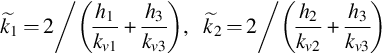
Define semipermeability
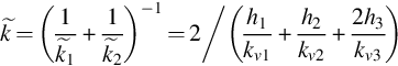
which is the semipermeability when the low-permeability layer is not treated as a layer in the model.
Since ![]() ,
, ![]() , from Eq. (8.1) we have
, from Eq. (8.1) we have ![]() . For simplicity, we take:
. For simplicity, we take:
where ![]() is calculated by Eq. (8.2).
is calculated by Eq. (8.2).
Suppose the initial pressure, pi, is constant everywhere. The well begins to produce from ![]() . Under these assumptions, the problem can be described mathematically as follows.
. Under these assumptions, the problem can be described mathematically as follows.
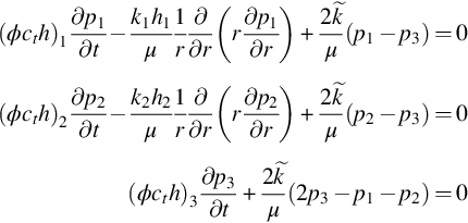
The initial conditions are
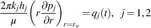
The boundary conditions at the well are
The boundary conditions at the well are
Infinitely thin skin for each layer is assumed:
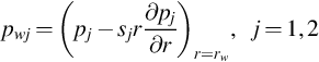
The flow rate, q2, of Layer 2, which flows to Layer 1 through the micro-annulus behind the casing, is described by a dimensionless function of pw1 and pw2:
Eq. (8.8) shows that we have assumed that the communication between the two productive layers can only happen when fluid flows through the skins of the two layers.
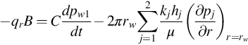
The apparent rate, q, of Layer 1, which is measured at the bottom of the well as a known function of time, should be the total rate of the two layers:
If the well produces at a constant surface rate qr, we have
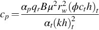
Instead of boundary condition Eq. (8.10a), Eqs. (8.4)–(8.10) give the complete mathematical description of the problem. To simplify the analysis, the following dimensionless parameters are used, which are similar to those used in reference Ehlig-Economides and Ayoub (1986):

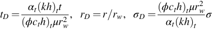

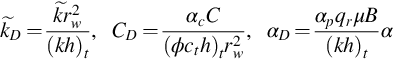
where
The values for αp, αt, and αc depend on the units used in the analysis. Values for several systems of units are given in Table 8.1.
Table 8.1
Unit Conversions
| Symbol | Customary Units | SI Metric Units | Darcy Units |
| q | STB/D | dm3/s | cm3/s |
| μ | cp | Pa. s | cp |
| k | md | μm2 | darcy |
| md/ft | μm2/m | darcy/cm | |
| r, h | ft | m | cm |
| p | psia | kPa | atm |
| t | hours | hours | s |
| ct | psia−1 | kPa−1 | atm−1 |
| C | bbl/psi | dm3/kPa | cm3/atm |
| αp | 141.2 | 106/2π | 1/2π |
| αt | .000264 | 3.6×10⁻⁶ | 1 |
| αc | .8936 | 159.2 | 1/2π |

Eqs. (8.1)–(8.10) are written in darcies. From Eqs. (8.14), (8.16), we have
8.3 The Interpretation Theory When q(t) is Known
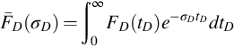
Suppose F(t) is a function of t. Its dimensionless form is given by
where αF is a constant, depending on what physical quality F(t) represents. Define the following dimension and dimensionless Laplace transformation:

and
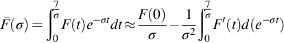
After integration by parts, Eq. (8.19) becomes

For simplicity, we also use ![]() for
for ![]() and
and ![]() for
for ![]() . From Eqs. (8.18) to (8.20) and Eq. (8.12), we have
. From Eqs. (8.18) to (8.20) and Eq. (8.12), we have

The dimensionless form of Eqs. (8.4)–(8.10) is given in Appendix F and solved in the Laplace space. We have the following governing equations of the problem from Appendix F:
where A(σD) and D(σD) are arbitrary functions, being determined by any two equations in Eqs. (8.22)–(8.25). Eigenvalue λj and coefficient αj are given by (F.23), (F.25). Function K(x) is
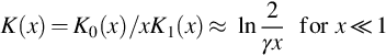
where ![]() . For most reservoirs and reasonable observation time, we have
. For most reservoirs and reasonable observation time, we have ![]() and
and ![]() . So we can use the approximation in Eq. (8.26).
. So we can use the approximation in Eq. (8.26).
The Laplace transform of a known function F(t) can be calculated approximately if the upper limit of the Laplace transform is taken as ![]() . Thus we can take
. Thus we can take
This integral can be calculated very quickly by the following formula:
where tj are net points in region ![]() .
.
When the leakage rate behind the casing is not negligible, both pw1 and pw2 change remarkably with time from the very beginning of production and are strongly influenced by all the parameters of the reservoir. This is quite different from case ![]() . From the previous works (Bremer et al., 1985; Ehlig-Economides and Ayoub, 1986; Lee et al., 1984; Wijesinghe and Kececioglu, 1988), which studied cases
. From the previous works (Bremer et al., 1985; Ehlig-Economides and Ayoub, 1986; Lee et al., 1984; Wijesinghe and Kececioglu, 1988), which studied cases ![]() , we know that in the short time period, the pressure pw1 of the active layer only depends on the parameters of the active layer and the observation pressure, pw2, will not change with time, as though the active layer did not produce. pw1 and pw2 gradually influence each other, and pw2 begins to change with time only after the short time period.
, we know that in the short time period, the pressure pw1 of the active layer only depends on the parameters of the active layer and the observation pressure, pw2, will not change with time, as though the active layer did not produce. pw1 and pw2 gradually influence each other, and pw2 begins to change with time only after the short time period.
We can make use of the communication rate between layers. For example, if there is no leakage behind the casing, we can use a specially designed leakage packer to create it in drawdown tests. The leakage rate, q2(t), through the leakage packer at a different time can be calculated by its function f(pw1,pw2), which is determined by the design and measured wellbore pressures, pw10(t) and pw20(t), in the test. If the middle layer of the reservoir is an impermeable one, that is ![]() , and a leakage packer is used, the two layers can be tested and interpreted by one drawdown test. This case will be studied later.
, and a leakage packer is used, the two layers can be tested and interpreted by one drawdown test. This case will be studied later.
Suppose we have obtained the expressions for ![]() and
and ![]() , which depend on σD and reservoir parameters and are different in different cases, pwD1 and pwD2 can be obtained by Stehfest's numerical inversion method. We construct the following objective function for nonlinear estimation of the reservoir parameters:
, which depend on σD and reservoir parameters and are different in different cases, pwD1 and pwD2 can be obtained by Stehfest's numerical inversion method. We construct the following objective function for nonlinear estimation of the reservoir parameters:

in real space or
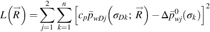
in Laplace space, where
If only one pressure, pw1 or pw2, is used in analysis, Eqs. (8.28), (8.29) should include one corresponding square term. ![]() or
or ![]() can be minimized to give the best parameter estimation, where
can be minimized to give the best parameter estimation, where ![]() is the dimensionless parameter vector being estimated. The parameters represented by vector
is the dimensionless parameter vector being estimated. The parameters represented by vector ![]() may be different for different cases and will be explained later in each case. In this chapter, we assume pi, (ϕcth)1, and (ϕcth)2 are known in all cases. Therefore, ω1 and ω2 are known parameters, they do not include in unknown parameters vector
may be different for different cases and will be explained later in each case. In this chapter, we assume pi, (ϕcth)1, and (ϕcth)2 are known in all cases. Therefore, ω1 and ω2 are known parameters, they do not include in unknown parameters vector ![]() , but, w1, s1, and s2 always do. Vector
, but, w1, s1, and s2 always do. Vector ![]() and (kh)t should be determined. Later we shall discuss how to choose the initial values of vector
and (kh)t should be determined. Later we shall discuss how to choose the initial values of vector ![]() in the nonlinear estimation. Barua and Horne (1988) discussed the different nonlinear parameter estimation methods used in well test analysis and compared them.
in the nonlinear estimation. Barua and Horne (1988) discussed the different nonlinear parameter estimation methods used in well test analysis and compared them.
8.3.1 Case for Known Function f(pw1,pw2)
Since the leakage function is dimensionless according to Eq. (8.9), for simplicity we use the same symbol f for f(pw1,pw2), f(pwD1,pwD2), f(t), and f(tD), though these four functions should have different forms because of the change of the independent variables.
Suppose pw1, pw2, and q(t) are measured in a drawdown test. The leakage function f(pw1,pw2) is known. Then, f(tD) is obtained by letting ![]() . Using Eq. (8.27),
. Using Eq. (8.27), ![]() and f(σD) can be calculated from f(tD) and q(t). From Appendix F we have
and f(σD) can be calculated from f(tD) and q(t). From Appendix F we have
which can be inverted numerically by Stehfest's method (1970) to obtain pwD1 and pwD2. The parameters being estimated are (kh)t, w1, s1, s2, and ![]() . Because f(tD) and q(t) may be different for different tests, and five parameters need to be estimated, the type curve match method is not suitable here.
. Because f(tD) and q(t) may be different for different tests, and five parameters need to be estimated, the type curve match method is not suitable here.
8.3.2 Case for Unknown Function f(pw1,pw2)
In most cases, the communication between layers is caused by micro-annulus behind the casing, the rate through which is unknown. What we know are, pw10, pw20, and q(t) measured in the test. The unknown leakage function f(tD) should be determined together with the reservoir parameters. Therefore, only equations Eqs. (8.23)–(8.25) can be used in this case. We can choose any two equations in Eqs. (8.23)–(8.25) to determine A(σD) and D(σD) and substitute them into the third equation to give calculated pressure or rate, which will be compared with its corresponding measured values to estimate the reservoir parameters. For example, we can choose pw1 to be compared, assuming that the theoretical q(t) and pw2 are exactly the same as their measured ones. Solving A(σD) and D(σD) from Eqs. (8.23), (8.25) and substituting into Eqs. (8.22), (8.24) results in the following:
where
pwD1 and f(tD) are obtained by numerical inversion of formulas Eqs. (8.31), (8.32). (kh)t, w1, s1, s2, ![]() are estimated by comparing pwD1 with pw10, using the nonlinear estimation method shown above.
are estimated by comparing pwD1 with pw10, using the nonlinear estimation method shown above.
8.3.3 Case for f=αD(pwD1−pwD2)
As Earlougher (1980) pointed out, the leakage rate q2 can be related with the micro-annulus's width Δr behind the casing and the pressure difference between the two layers. As ratio rw/Δr increases, the leakage flow through the micro-annulus will obey Poiseuille's law for closely spaced parallel plates, that is,

Therefore, it is reasonable to approximate the leakage rate by
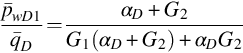
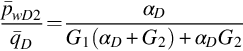
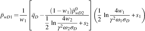
It is not difficult to design a leakage packer through which flow will obey Eq. (8.34). If function f has the linear form Eq. (8.34), from Eqs. (F.31), (F.32) in Appendix F we have


where

Eqs. (8.35), (8.36) show that in Laplace space, rate-normalized pressures are independent of flow rate and only depend on reservoir parameters. We can use pw1 and/or pw2 in parameter estimation, depending on if pw10 and/or pw20 are measured together with q(t) during the testing. For example, we can measure only q(t) and pw10(t) and compare pw10 with pwD1, calculated by Eq. (8.35), to determine reservoir parameters. αD will be estimated together with other parameters if it is unknown.
8.3.4 Case 
The study of case ![]() is important, because the behavior of the reservoir with
is important, because the behavior of the reservoir with ![]() in the short time period is the same as those with
in the short time period is the same as those with ![]() and thus the results of the latter can also be used for the former.
and thus the results of the latter can also be used for the former.
When ![]() , from Eqs. (F.40), (F.41), and Eq. (8.43) we have
, from Eqs. (F.40), (F.41), and Eq. (8.43) we have
and
In the dimension form, the above equations become

Eqs. (8.38), (8.39) show that in Laplace space rate-normalized pressures of both layers are straight lines on the semilog plot. If q(t) and f(tD) are known, we can determine k1h1, k2h2, s1, s2 from the slope and intercept of Eqs. (8.38), (8.39).
When ![]() , we still can analyze the early time data as for the case when
, we still can analyze the early time data as for the case when ![]() and give an approximate estimation of the layer parameters, which are taken as the initial guess of the layer parameters used in the nonlinear estimation and are corrected by it.
and give an approximate estimation of the layer parameters, which are taken as the initial guess of the layer parameters used in the nonlinear estimation and are corrected by it.
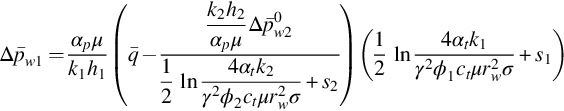
If f(tD) has the linear form of Eq. (8.34) with unknown coefficient αD, (F.42), (F.43) results in
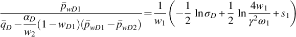
In case pw1, pw2, and q(t) are measured in the testing, we can determine αD/w2 and s2 from the slope and intercept of Eq. (8.40a). Using the obtained αD/w2 in Eq. (8.41a), w1 and s1 can be determined by the trial-and-error method or any other method.
Then ![]() .
.
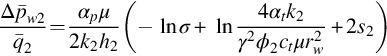
In the dimension form, the above equations become
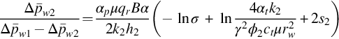

Therefore, α/k2h2 and s2 can be determined by Eq. (8.40b). The correct value of α should make the plot of ![]() versus ln σ a straight line. So σ is determined by the trial-and-error method or other methods. k1h1 and s1 are determined by the slope and intercept of Eq. (8.41b).
versus ln σ a straight line. So σ is determined by the trial-and-error method or other methods. k1h1 and s1 are determined by the slope and intercept of Eq. (8.41b).
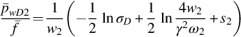
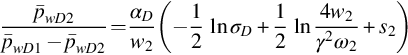
Eqs. (8.40a), (8.41a) can be changed into
and
where

If only one wellbore pressure, pw1 or pw2, is measured together with rate q(t), then Eqs. (8.42a) or (8.42b) can be used to estimate reservoir parameters (kh)t, w1, s1, s2, and αD. This is the most difficult case, because five parameters need to be estimated by the matching of only one pressure and we don't have a good way to give an initial guess of these parameters yet.
If we don't have any knowledge about function f(pw1,pw2), we use pw1 as the matching pressure, assuming the measured pw20 is equal to the theoretical one. Substituting Eq. (8.39) into Eq. (8.38), we have
or
Inverse it to obtain pwD1 or Δpw1, which will be used to estimate (kh)t, w1, s1, and s2 by the nonlinear estimation method. Function f(tD) is calculated by Eqs. (8.38) or (8.39) after the above parameters are estimated.
In order to give an initial guess of parameters (kh)t, w1, s1, and s2, which will be refined by the nonlinear estimation, we take the linear form, Eq. (8.34), as the first approximation of f(pw1,pw2). Then the initial values of the parameters can be calculated by Eqs. (8.40), (8.41).
8.4 The Interpretation Theory When the Well Produces with a Constant Surface Rate
In practice, the most important case in well testing is the surface rate of the well being constant. Although the surface rate of the well is constant, the bottom hole rate changes with time because of the wellbore storage. From Appendix G we know that the Laplace transform of the changing bottom hole rate can be written as

which was obtained by other authors before. Substituting Eq. (8.45) into the previous results for the changing rate, q(t), we can obtain parallel results for the constant surface rate, as it was done in Appendix G.
8.4.1 Case for Known Function f(pw1, pw2)
In this case, both pw1 and pw2 can be used in parameter estimation. From Appendix G we have

which will be used in nonlinear estimation to determine (kh)t, w1, s1, s2, ![]() , and CD. L1 and L2 are given by Eq. (G.6).
, and CD. L1 and L2 are given by Eq. (G.6).
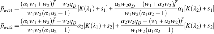
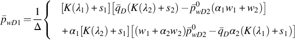
8.4.2 Case for Unknown Function f(pw1, pw2)
In this case only one pressure can be used in nonlinear parameter estimation, assuming the other one is the same as its measured value. We choose pw1 as the pressure for matching. From Appendix G we have
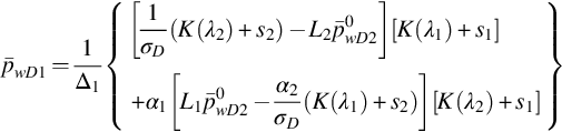
and
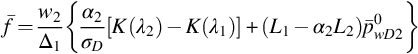
where
The parameters being estimated by the match of pw1 are (kh)t, w1, s1, s2, ![]() , and CD.
, and CD. ![]() is calculated by Eq. (8.48) after the parameter estimation.
is calculated by Eq. (8.48) after the parameter estimation.
8.4.3 Case for f=αD(pwD1−pwD2)
In this case, pw1 and/or pw2 can be used for nonlinear estimation. From Appendix G we have

Comparing pw10 with pwD1 and/or pw20 with pwD2, we can see that the parameters (kh)t, w1, s1, s2, ![]() , αD, and CD can be determined according to Eq. (8.50).
, αD, and CD can be determined according to Eq. (8.50).
8.4.4 Case for 
From Appendix G we have
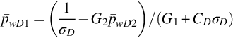
and
If function f is unknown, we must assume ![]() and estimate parameters (kh)t, w1, s1, s2, and CD by comparing pw10 with pwD1, which is calculated from Eq. (8.51). Function f is determined by Eq. (8.52).
and estimate parameters (kh)t, w1, s1, s2, and CD by comparing pw10 with pwD1, which is calculated from Eq. (8.51). Function f is determined by Eq. (8.52).
If ![]() , from Eqs. (8.51), (8.52), we have Eq. (8.40), and
, from Eqs. (8.51), (8.52), we have Eq. (8.40), and

If pw1 and pw2 are measured simultaneously in the test, α/k2h2 and s2 can be obtained from Eq. (8.40) as before. α, k1h1, s1, and CD are estimated by Eq. (8.53), using the nonlinear estimation method.
Eqs. (8.53), (8.40) can be changed as follows:
and
If only one pressure, pw1 or pw2, is measured in the test, Eqs. (8.54) or (8.55) can be used in the nonlinear estimation to determine parameters (kh)t, w1, s1, s2, αD, and CD.
8.4.5 Limiting Behavior for f=αD(pwD1−pwD2)
In the short time period, the transient flow behaves as though ![]() . Therefore, pressure pw1 and pw2 are given by Eqs. (8.40), (8.53) or equivalently by Eqs. (8.54), (8.55).
. Therefore, pressure pw1 and pw2 are given by Eqs. (8.40), (8.53) or equivalently by Eqs. (8.54), (8.55).
In the long time period, that is, for ![]() , the wellbore pressures can be approximated by
, the wellbore pressures can be approximated by

where
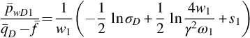
From Eq. (8.56) we have
Thus, in the long time period, pwD1(tD) and pwD2(tD) are parallel semilog straight lines with one-half slope, which will determine (kh)t, and pressure difference, ![]() , is a constant. If we let
, is a constant. If we let ![]() ,
, ![]() in Eq. (8.58) and
in Eq. (8.58) and ![]() ,
, ![]() in Eq. (7.22) of Chapter 7, the two equations become identical. We see that the influence of fluid compressibility of the low-permeability middle layer on the wellbore pressure of the two high-permeability layers in the long time period is indicated by subtracting a constant
in Eq. (7.22) of Chapter 7, the two equations become identical. We see that the influence of fluid compressibility of the low-permeability middle layer on the wellbore pressure of the two high-permeability layers in the long time period is indicated by subtracting a constant ![]() from the wellbore pressures. Physically, this is a very natural result. Because of the expansion of the fluid in the low-permeability middle layer during drawdown testing, the pressure drops in the two high-permeability layers should be smaller. Constant
from the wellbore pressures. Physically, this is a very natural result. Because of the expansion of the fluid in the low-permeability middle layer during drawdown testing, the pressure drops in the two high-permeability layers should be smaller. Constant ![]() is the amount of dimensionless pressure drop in the two high-permeability layers caused by fluid expansion in the low-permeability layer. Noticing
is the amount of dimensionless pressure drop in the two high-permeability layers caused by fluid expansion in the low-permeability layer. Noticing ![]() , we can write
, we can write ![]() in Eq. (8.56). This shows that ω3 is on an equality with ω1 or ω2 in the long time period. This is highly intuitive physically. Another interesting result from Eq. (8.58) is that pressure difference,
in Eq. (8.56). This shows that ω3 is on an equality with ω1 or ω2 in the long time period. This is highly intuitive physically. Another interesting result from Eq. (8.58) is that pressure difference, ![]() , is independent of ω3 in the long time period, though pw1 and pw2 are not.
, is independent of ω3 in the long time period, though pw1 and pw2 are not.
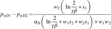
Solving Eq. (8.58) for ![]() , we have
, we have

If we let ![]() in Eq. (8.59) and
in Eq. (8.59) and ![]() ,
, ![]() in Eq. (7.24) of Chapter 7, the two equations become identical.
in Eq. (7.24) of Chapter 7, the two equations become identical.
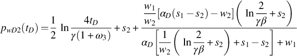
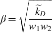
![]() can also be determined by any point on the semilog straight lines given by Eq. (8.56). For example, let tD be tpD in Eq. (8.56), where tpD is the total production time in the drawdown period. Solving for β and using Eq. (8.57), we have
can also be determined by any point on the semilog straight lines given by Eq. (8.56). For example, let tD be tpD in Eq. (8.56), where tpD is the total production time in the drawdown period. Solving for β and using Eq. (8.57), we have

where
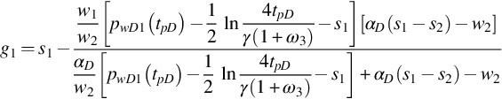
and
where
Therefore, semipermeability ![]() can be calculated from one of the two wellbore pressures at the end of the drawdown test, if the other parameters have been estimated.
can be calculated from one of the two wellbore pressures at the end of the drawdown test, if the other parameters have been estimated.
In the long time period, the total rate of the well and the leakage rate q2 will become steady when the wellbore storage effect dies out. The steady leakage rate qD2 is

Then,

The leakage rates, calculated by Eq. (8.64), conform well with the simulation results in the long time period.
8.4.6 Buildup Case
Suppose the well is shut-in at time tp, which is long enough to make the wellbore pressures satisfy Eq. (8.56). From the superposition principle, the pressure in the buildup period is ![]() , where
, where ![]() satisfies Eq. (8.56).
satisfies Eq. (8.56).
Using Eq. (8.56), we have

where pwDj(tD) is calculated by the method given above for drawdown. In the short buildup period, we have ![]() . Eq. (8.66) can be simplified to
. Eq. (8.66) can be simplified to
So buildup can be analyzed like drawdown. In the long time buildup period, we have ![]() . Eq. (8.66) becomes
. Eq. (8.66) becomes
It is a straight line on the Horner plot with one-half slope, which determines (kh)t.
8.4.7 The Determination of Initial Values for Nonlinear Parameter Estimation
Suppose ![]() are known. The parameters to be estimated are k1h1, k2h2, s1, s2,
are known. The parameters to be estimated are k1h1, k2h2, s1, s2, ![]() , CD, αD or function f(pw1,pw2). If the communication between layers is caused by a leakage packer and f(pw1,pw2) is known, we cut αD and f(pw1,pw2) from the parameter list. Six or more parameters need to be estimated, so the best way to estimate these parameters is the nonlinear estimation method, which needs a good initial value to start; otherwise it might fail. We now discuss how to choose the initial values for these parameters.
, CD, αD or function f(pw1,pw2). If the communication between layers is caused by a leakage packer and f(pw1,pw2) is known, we cut αD and f(pw1,pw2) from the parameter list. Six or more parameters need to be estimated, so the best way to estimate these parameters is the nonlinear estimation method, which needs a good initial value to start; otherwise it might fail. We now discuss how to choose the initial values for these parameters.
We first consider the case when both pw1 and pw2 are measured simultaneously in the test. We know that interlayer crossflow will not influence the behavior of the system in the short time period. So the formula for case ![]() can be used to analyze the early data of the test. If function f(pw1,pw2) is known, we can use Eq. (8.52) to determine k2h2, and s2; we can use Eq. (8.51) to determine k1h1, s1, and CD; and we can use Eq. (8.59) to determine
can be used to analyze the early data of the test. If function f(pw1,pw2) is known, we can use Eq. (8.52) to determine k2h2, and s2; we can use Eq. (8.51) to determine k1h1, s1, and CD; and we can use Eq. (8.59) to determine ![]() .
.
If f(pw1,pw2) is unknown, we can take the linear form, Eq. (8.34), as the first approximation and use Eq. (8.53) to determine αD, CD, k1h1, and s1, k2h2, s2, and ![]() are determined as above. Therefore, the parameters of the two layers can be estimated separately when pw1 and pw2 are measured simultaneously in the testing. The obtained parameters k1h1, k2h2, s1, s2,
are determined as above. Therefore, the parameters of the two layers can be estimated separately when pw1 and pw2 are measured simultaneously in the testing. The obtained parameters k1h1, k2h2, s1, s2, ![]() , and CD, are then used in the nonlinear parameter estimation as initial values and refined. Lastly, function f is calculated by Eq. (8.48), using the refined parameters.
, and CD, are then used in the nonlinear parameter estimation as initial values and refined. Lastly, function f is calculated by Eq. (8.48), using the refined parameters.
We now consider the case when only one wellbore pressure, pw1 or pw2, is measured in the test; ![]() can be determined by one wellbore pressure at time tp, using Eqs. (8.60) or (8.62) after the other parameters are determined. (kh)t can be determined by the slope of Eq. (8.56), using the measured wellbore pressure at the long time period. The other parameters, w1, s1, s2, αD, and CD, have to be estimated by the nonlinear estimation method, which compares pw1 or pw2, calculated by Eq. (8.50), with pw10 or pw20. This is the most difficult case, because these parameters cannot be estimated separately and we do not have a good way to choose initial values for them to start the nonlinear estimation. To diminish this difficulty, the wellbore storage coefficient, CD, can be estimated independently from the well structure data and take it as an initial value, which can also be used in the case when both pw1 and pw2 are measured. The initial values of w1, s1, s2, and αD have to be given according to our experiences and judgement.
can be determined by one wellbore pressure at time tp, using Eqs. (8.60) or (8.62) after the other parameters are determined. (kh)t can be determined by the slope of Eq. (8.56), using the measured wellbore pressure at the long time period. The other parameters, w1, s1, s2, αD, and CD, have to be estimated by the nonlinear estimation method, which compares pw1 or pw2, calculated by Eq. (8.50), with pw10 or pw20. This is the most difficult case, because these parameters cannot be estimated separately and we do not have a good way to choose initial values for them to start the nonlinear estimation. To diminish this difficulty, the wellbore storage coefficient, CD, can be estimated independently from the well structure data and take it as an initial value, which can also be used in the case when both pw1 and pw2 are measured. The initial values of w1, s1, s2, and αD have to be given according to our experiences and judgement.
8.5 The Influence of Different Parameters on Drawdown Curves
Using the above formulas in Laplace space for wellbore pressures and Stehfest's numerical inversion algorithm, we can calculate pressures and rates at different times. The simulation results for some reservoir parameters are shown in Figs. 8.1–8.11, assuming the well produces with a constant surface rate.
8.5.1 The Influence of the Linear Leakage Rate on Wellbore Pressure
Figs. 8.1–8.3 show the influence of the linear leakage rate on wellbore pressure. Fig. 8.1 shows that the drawdown curves for both active and observation layers will have two straight lines on the semilog plot for ![]() . Similar to the no-leakage case, the slope of the second straight line is one-half. But the slope of the first straight line changes with the leakage coefficient αD. pw1 and pw2 will get close to each other when αD increases.
. Similar to the no-leakage case, the slope of the second straight line is one-half. But the slope of the first straight line changes with the leakage coefficient αD. pw1 and pw2 will get close to each other when αD increases.

 . (After Gao, (1989) SPE 19444, Permission to publish by the SPE, Copyright SPE.)
Figs. 8.2 and 8.3 are the semilog plot and log–log plot for the same cases when ![]() . Fig. 8.2 shows that the first straight line in the semilog plot does not appear because of the wellbore storage effect. The second straight lines with one-half slope appear in the long time period when the wellbore storage effect died out. Fig. 8.3 shows that the leakage coefficient αD influences not only the wellbore pressure, but also the pressure derivative.
. Fig. 8.2 shows that the first straight line in the semilog plot does not appear because of the wellbore storage effect. The second straight lines with one-half slope appear in the long time period when the wellbore storage effect died out. Fig. 8.3 shows that the leakage coefficient αD influences not only the wellbore pressure, but also the pressure derivative.
 . (After Gao (1989) SPE 19444, Permission to publish by the SPE, Copyright SPE.)
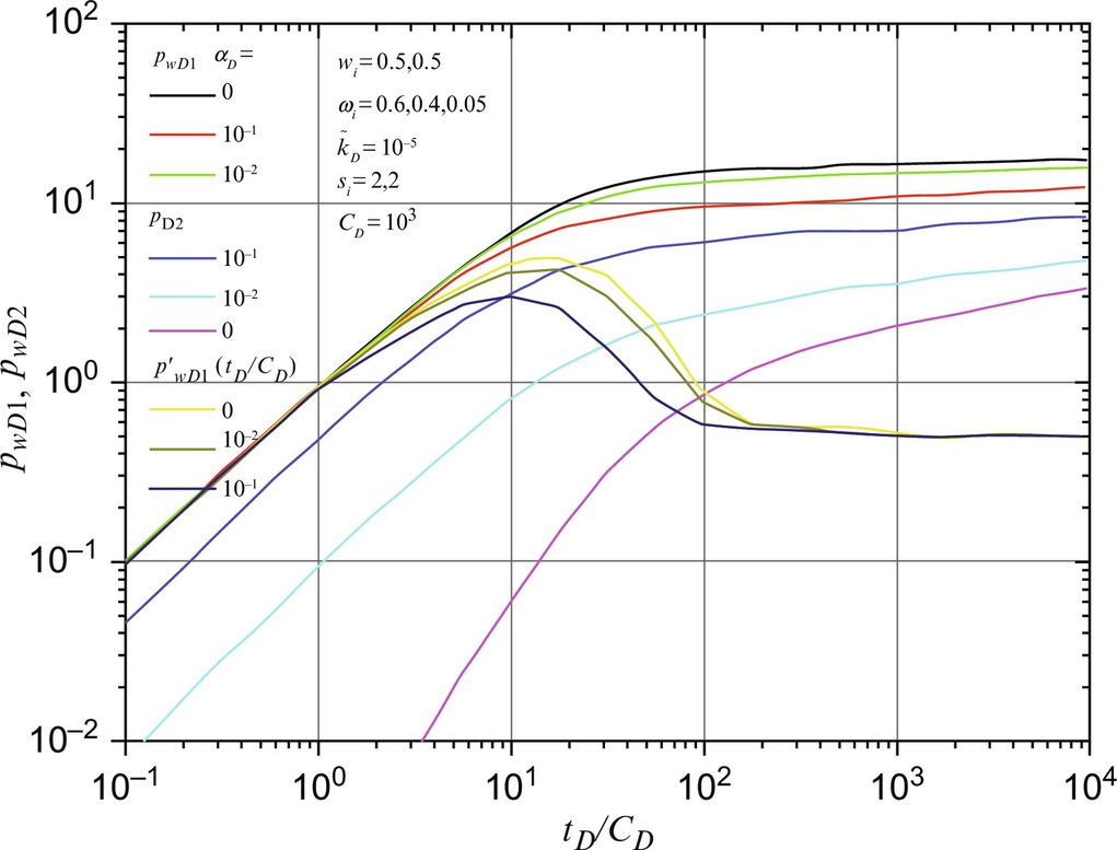
8.5.2 The Influence of Storativity of the Low-Permeability Layer on Wellbore Pressure
Fig. 8.4 shows the influence of storativity ω3 on the wellbore pressure. When ω3 becomes larger, the pressure drops in Layers 1 and 2 are smaller; that is, both pwD1 and pwD2 decrease when ω3 increases. The influence of ω3 on pwD2 can be seen clearly on the figure. The influence of ω3 on pwD1 is so small that we can see it from the simulation results but hardly can express it on this figure. The case for ![]() is equivalent to the steady crossflow modle. Therefore, Fig. 8.4 also gives a comparison of the steady crossflow modle with the semipermeable wall modle when storativity ω3 is considered. Wijesinghe and Kececioglu (1988) compared the steady crossflow modle with the unsteady crossflow modle and obtained same conclusions about the influence of storativity ω3. They also found the influence of ω3 is mainly on the observation pressure; its influence on active pressure, pw1, is very small. Eq. (8.56) shows that pwD1 and pwD2 will decrease by
is equivalent to the steady crossflow modle. Therefore, Fig. 8.4 also gives a comparison of the steady crossflow modle with the semipermeable wall modle when storativity ω3 is considered. Wijesinghe and Kececioglu (1988) compared the steady crossflow modle with the unsteady crossflow modle and obtained same conclusions about the influence of storativity ω3. They also found the influence of ω3 is mainly on the observation pressure; its influence on active pressure, pw1, is very small. Eq. (8.56) shows that pwD1 and pwD2 will decrease by ![]() in the long time period, compared with those when
in the long time period, compared with those when ![]() . This is also proved to be true by the numerical results.
. This is also proved to be true by the numerical results.

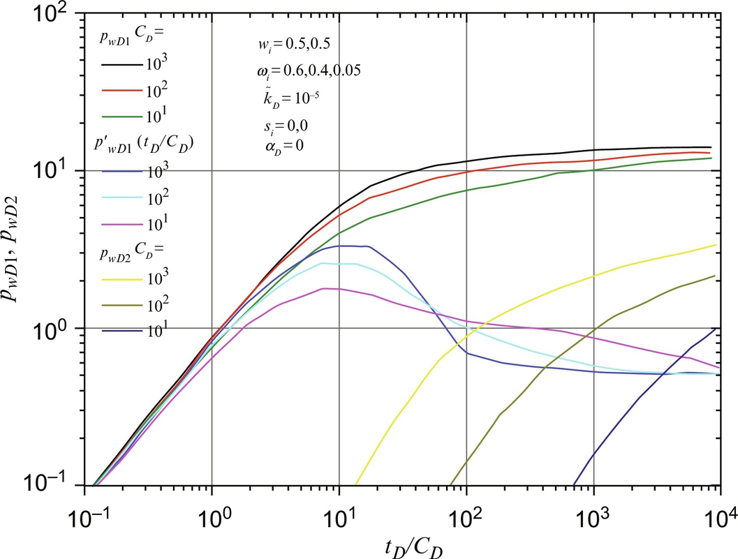
8.5.3 The Influence of Wellbore Storage on Wellbore Pressure
Fig. 8.5 shows the influence of the wellbore storage effect on wellbore pressure and its derivative when crossflow exists and ω3 is not zero. We see the change of the pressure derivative of the active layer with CD is quite different from that for a single layer reservoir. The derivative curve for large CD is above the curve for small CD at the short time and below it at the long time.
8.5.4 The Influence of Semipermeability on Wellbore Pressure
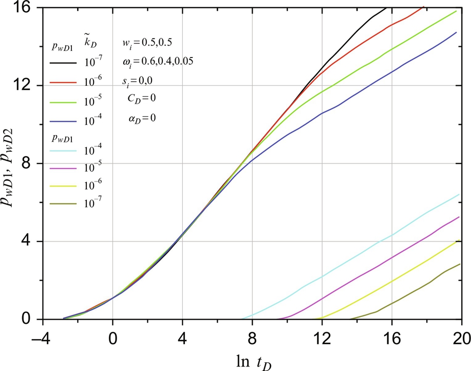
Fig. 8.6 shows the influence of semipermeability, ![]() , when αD and CD are zero. In the short time period, pwD2 is equal to zero and pwD1 shows a first straight line on semilog plot. The first straight line of pwD1 grows longer when
, when αD and CD are zero. In the short time period, pwD2 is equal to zero and pwD1 shows a first straight line on semilog plot. The first straight line of pwD1 grows longer when ![]() is smaller and has a slope of
is smaller and has a slope of ![]() . In the long time period, both pwD1 and pwD2 are parallel straight lines with one-half slope.
. In the long time period, both pwD1 and pwD2 are parallel straight lines with one-half slope.
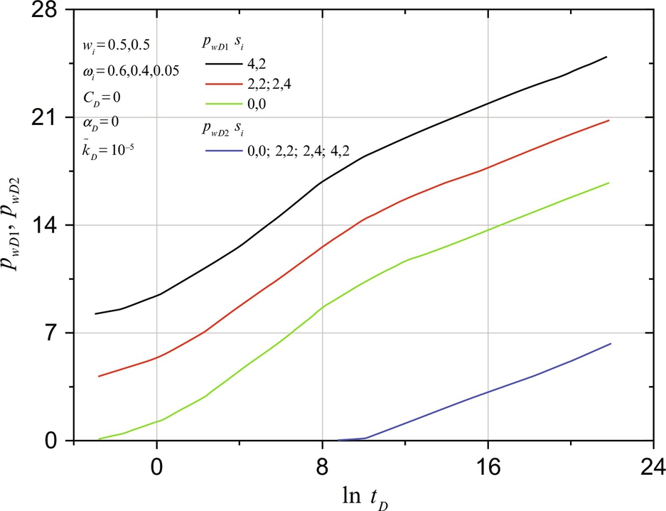
8.5.5 The Influence of Skin Factor on Wellbore Pressure
Figs. 8.7 and 8.8 show the influence of skin factors of the two layers. When leakage rate and wellbore storage effect do not exist, the skin factor, s1, of the active layer will cause the curve of pwD1 to move in a vertical direction; the skin factor, s2, of the closed layer does not have any influence on the problem. When the leakage behind the casing exists, both pwD1 and pwD2 increase with the increase of s2. From the simulation results we see that the leakage rate, qD2, will decrease with the increase of s2, since stronger resistance to flow in Layer 2 is created by a larger value of s2. Thus, when the skin factor s2 is larger, the leakage rate q2 and the pressure drop in Layer 2 are smaller. On the contrary, wellbore pressure pw2 will increase when s2 increases. The reason is that pw2 is the sum of the pressure at the wall of the well and the pressure drop through the skin of Layer 2. A larger skin factor s2 causes a bigger pressure drop through the skin. This pressure drop will exceed the increase of pressure in Layer 2 caused by the increase of the skin factor s2, so pressure pw2 will decrease when s2 increases.
 . (After Gao (1989) SPE 19444, Permission to publish by the SPE, Copyright SPE.)
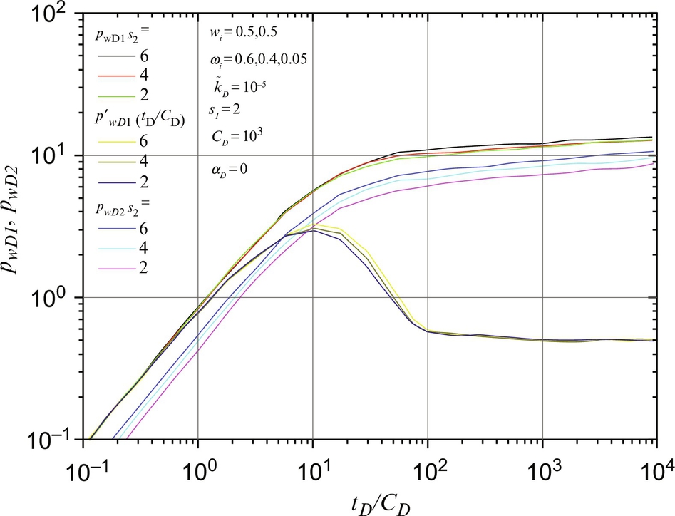 . (After Gao (1989) SPE 19444, Permission to publish by the SPE, Copyright SPE.)
8.5.6 The Influence of w1 on Wellbore Pressure
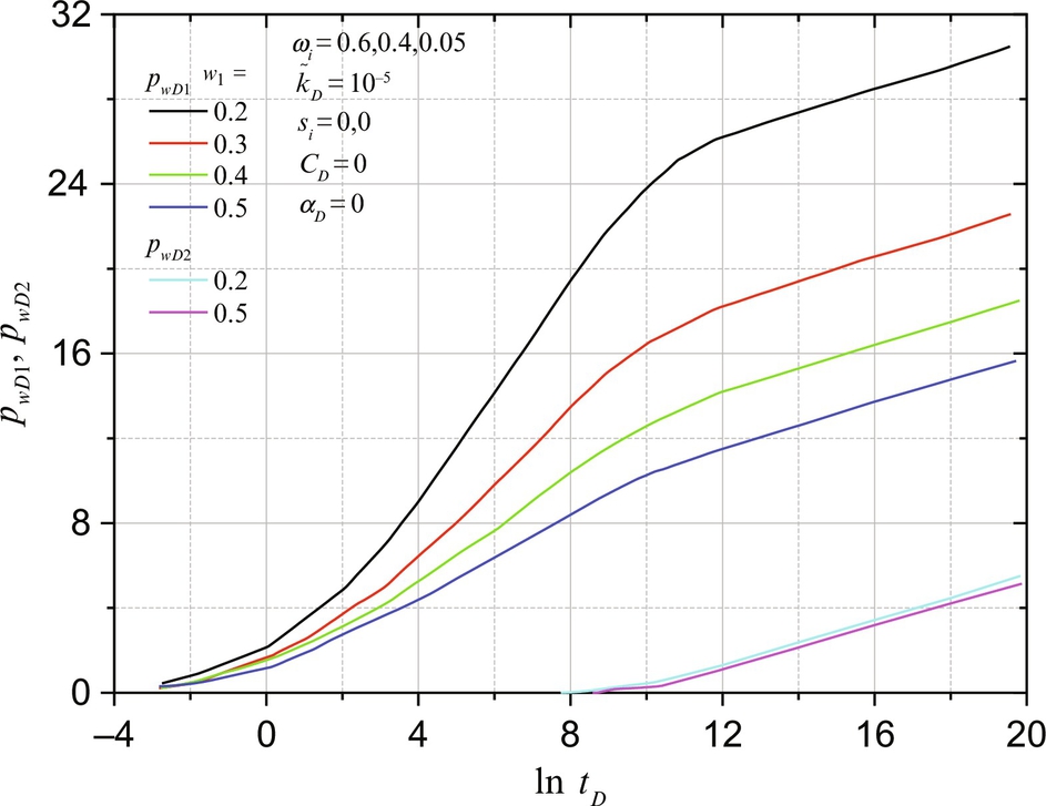
Fig. 8.9 shows the influence of w1 when there is no-leakage behind the casing and wellbore storage effect. We see the semilog curves of pwD1 have two straight lines with the first slope being ![]() and the second slope being
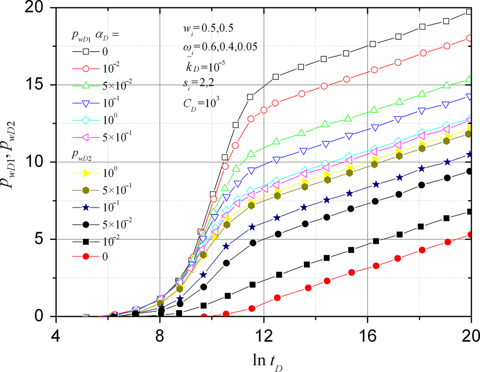
and the second slope being ![]() . pwD2 has a straight line with one-half slope in the long time period. The pressure of the active layer, pwD1, changes greatly with w1 while the observation pressure, pwD2, hardly can be influenced by w1. Fig. 8.10 shows the influence of w1 on pwD1 and pwD2 when the leakage rate and wellbore storage effect exist. The plot is made of θj against ln σD, where
. pwD2 has a straight line with one-half slope in the long time period. The pressure of the active layer, pwD1, changes greatly with w1 while the observation pressure, pwD2, hardly can be influenced by w1. Fig. 8.10 shows the influence of w1 on pwD1 and pwD2 when the leakage rate and wellbore storage effect exist. The plot is made of θj against ln σD, where

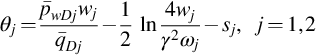
The curves give a common straight line with one-half slope when σD is not very small. This means the approximate equations, Eqs. (8.38a), (8.39a), are correct. The curves deviate from straight ![]() for
for ![]() . Eqs. (8.38a), (8.39a) can be derived from Eqs. (F.40), (F.41), which is not suitable for large σD. This approximation causes the deviation at large σD. The deviation from the straight line at small σD is caused by the interlayer crossflow between layers. The curves deviate from the straight line upward for Layer 2 and downward for Layer 1. We also noticed that the straight line portion for Layer 1 is much longer than that for Layer 2.
. Eqs. (8.38a), (8.39a) can be derived from Eqs. (F.40), (F.41), which is not suitable for large σD. This approximation causes the deviation at large σD. The deviation from the straight line at small σD is caused by the interlayer crossflow between layers. The curves deviate from the straight line upward for Layer 2 and downward for Layer 1. We also noticed that the straight line portion for Layer 1 is much longer than that for Layer 2.
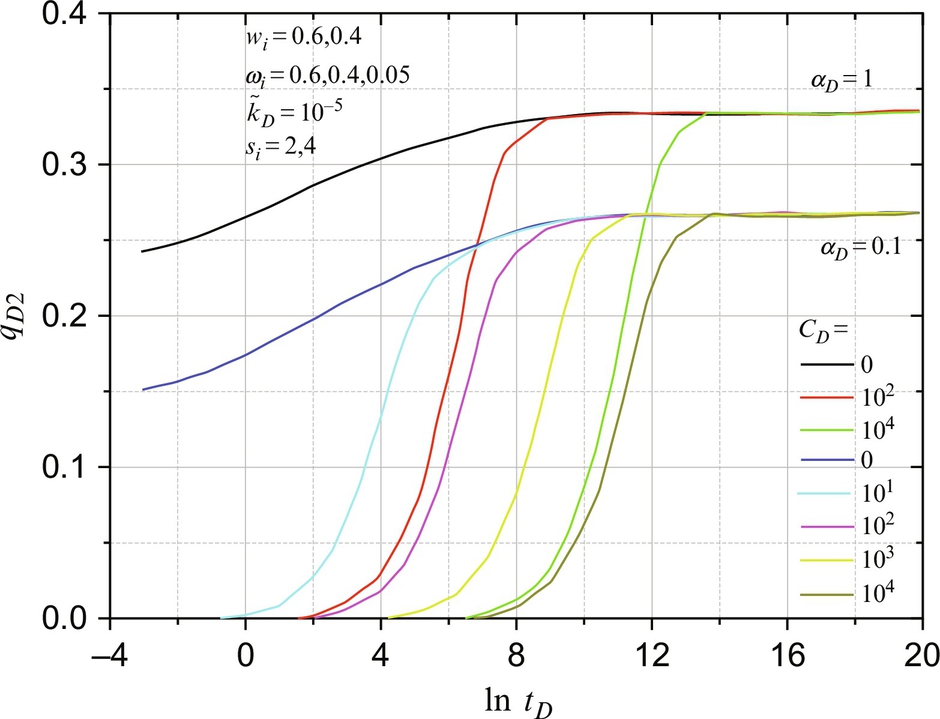
8.5.7 The Influence of Leakage Rates on Wellbore Pressure
Fig. 8.11 shows the leakage rates, qD2, at different CD and αD. We see qD2 always converges to a steady leakage rate in different cases. The wellbore storage effect only influences the convergent time, but it cannot change the steady leakage rate. The steady leakage rate is determined by Eq. (8.64), which conforms well to simulation results.
8.6 Summary
An interpretation theory for the vertical interference tests in a three-layer reservoir is given, which includes the skin factor of each layer, wellbore storage effect, interlayer crossflow, leakage rate behind the pipe, storativity of the low-permeability middle layer, and variable production rate. The inclusion of the storativity of the low-permeability middle layer makes the calculated pressures for both the active and the observation layers from the theory very close to the measured pressures, so it makes the interpretation more reliable. The inclusion of the leakage behind the casing makes it possible to use the vertical interference test data of a well that is poorly cemented and interpret reservoir parameters from it.
(1) The reservoir parameters can be interpreted by the equations in Laplace space as well as by those in real-time space. In Laplace space, rate-normalized wellbore pressure will show out a first semilog straight line, which could be used to determine the kh value and skin factor for each layer.
(2) If the wellbore pressures of both the active layer and the observation layer are measured in the tests, it is possible to interpret the unknown reservoir parameters and the leakage rate as a function of time simultaneously by the nonlinear estimation method. If the leakage rate behind the pipe is directly proportional to the pressure difference, ![]() , between the active and observation layers, both pw1 and pw2 can be used to compare with the measured pressures. In this case, the parameters of the two layers can be estimated separately.
, between the active and observation layers, both pw1 and pw2 can be used to compare with the measured pressures. In this case, the parameters of the two layers can be estimated separately.
(3) If a well produces with a constant surface rate, the leakage rate will eventually become steady. The wellbore storage effect will not influence the steady leakage rate; it only influences the time to reach this steady rate.
(4) The storativity of the low-permeability middle layer will mainly influence the observation pressure in the middle time period. In the long time period, the pressures in both the active layer and the observation layer will increase a constant amount because of the fluid expansion in the middle layer.
(5) For the vertical interference testing in a three-layered reservoir, there are many factors that influence not only the shape of the wellbore pressure curves, but also the shape of pressure derivative curves, such as wellbore storage effect, leakage behind the casing, skin factors, storativity of each layer, semipermeability between layers, and kh product. The interpretation methods, using semilog straight lines or type curve matching, can only give a rough estimation of the reservoir parameters. The best way to estimate reservoir parameters might be the nonlinear estimation method.