Approximate Solution of the Diffusivity Crossflow Problem in n-Layer Reservoirs (Chapter 3)
Suppose a well produces from all layers in an n-layer reservoir at a common wellbore pressure and a constant total rate, q, for t>0 . Under the assumptions we made, the problem can be described as follows. The equations are
1ηi∂pi∂t−1r∂∂r(r∂pi∂r)+k˜i−1kihi(pi−pi−1)+k˜ikihi(pi−pi+1)=0,i=1,2,…,n;k˜0=k˜n=0
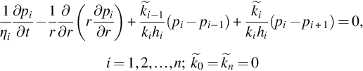 (B.1)
(B.1)
where ηi=kiϕiμct and k˜
 is the semipermeability between layers i and layers i+1
 .
.
The boundary conditions at the well are mixed, in other words, common to all layers. The flow conditions are
∑i=1n2πkihiμ(r∂pi∂r)r=rw=qB
 (B.2a)
for t>0,
p1(rw,t)=p2(rw,t)=⋯=pn(rw,t)
 (B.2b)
for t>0,
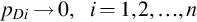
pi→p0,i=1,2,…,n
 (B.2c)
when r→∞ , and
, and
pi→p0,i=1,2,…,n
(B.3)
when t→0 .
.
Using the dimensionless quantities given in Eqs. (3.1), (3.2), the problem becomes
1ηDi∂pDi∂tD−1rD∂∂rD(rD∂pDi∂rD)+1wi[k˜Di−1(pDi−pDi−1)+k˜Di(pDi−pDi+1)]=0,k˜D0=k˜Dn=0;i=1,2,…,n
 (B.4)
(B.4)
∑i=1nwi(rD∂pDi∂rD)rD=1=−∑i=1nqDi=−1
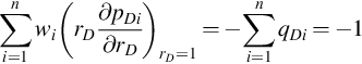 (B.5a)
pD1(1,tD)=pD2(1,tD)=⋯=pDn(1,tD)
 (B.5b)
pDi→0,i=1,2,…,n
 (B.5c)
when rD→∞
pDi→0,i=1,2,…,n
(B.6)
The new dependent variables are
pD=∑i=1nwipDi
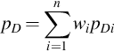 (3.4a)
and
ΔpDi=pDi−pDi+1,i=1,2,…,n−1
 (3.4b)
pDi can be expressed in terms of pD and ΔpDi as
pDi=pD+∑j=1n−1(1−wsj)ΔpDj−∑j=1i−1ΔpDj,i=1,2,…,n
 (B.7)
(B.7)
where
wsi=∑j=1iwj,i=1,2,…,n
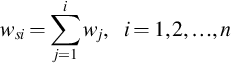 (3.15)
Subtracting Eq. (B.4) for layer i+1 from Eq. (B.4) for layer i and using Eq. (3.4b), we get
∂∂tD(pDiηDi−pDi+1ηDi+1)−1rD∂∂rD(rD∂ΔpDi∂rD)−k˜Di−1wiΔpDi−1+k˜Di(1wi+1wi+1)ΔpDi−k˜Di+1wi+1ΔpDi+1=0,k˜D0=k˜Dn=0;i=1,2,…,n−1
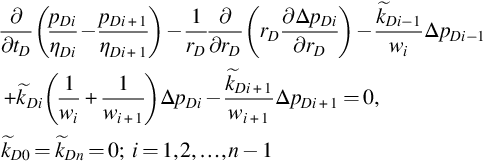 (B.8a)
Multiplying Eq. (B.4) for layer i by wi and adding, we get
∂∂tD(∑j=1nwiηDipDi)−1rD∂∂rD(rD∂pD∂rD)=0
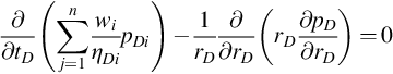 (B.8b)
The boundary conditions in Eq. (B.5) become
(rD∂pD∂rD)rD=1=−1
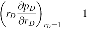 (B.9a)
ΔpDi(1,tD)=0,i=1,2,…,n−1
 (B.9b)
and
pD→0,ΔpDi→0,i=1,2,…,n−1
 (B.9c)
when rD→∞. The initial conditions in Eq. (B.6) become
pD→0,ΔpDi→0,i=1,2,…,n−1
(B.10)
when tD→0 . Because the wellbore pressure and initial pressure for all layers are the same and crossflows exist, the pressure differences ΔpDi,i=1,2,…,n−1
 should be very small compared with pD, when time is not very short. This fact is confirmed by the numerical calculation. The approximate solution for pD is obtained by neglecting all ΔpDi in Eq. (B.8b), compared with pD. Using Eqs. (B.7), (3.3), we get
∂pD∂tD−1rD∂∂rD(rD∂pD∂rD)=0
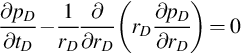 (B.11)
Using boundary conditions in Eq. (B.9) and initial conditions in Eq. (B.10), the approximate solution of Eq. (B.11) is pD=−12Ei(−ξ) , where ξ=r2D4tD
 is the effective Boltzmann variable and Ei is the exponential integral function, defined by
−Ei(−ξ)=∫∞ξe−uudu
To obtain the asymptotic solution for ΔpDi, we substitute Eq. (3.10) into Eq. (B.7) and place the result into Eq. (B.8a) and neglect all derivatives of ΔpDi. This produces the following algebraic equations for determining ΔpDi,i=1,2,…,n−1 :
:
−k˜DiwiΔpDi−1+k˜Di(1wi+1wi+1)ΔpDi−k˜Di+1wi+1ΔpDi+1=−Di2tDe−ξ,k˜D0=k˜Dn=0;i=1,2,…,n−1
 (B.12)
where, Di=1ηDi−1ηDi+1,i=1,2,…,n−1 . Let
. Let
ΔpDi=αsie−ξtD,i=1,2,…,n−1
 (B.13)
Substituting into Eq. (B.12) and canceling e−ξtD , we get
−k˜Di−1wiαsi−1+k˜Di(1wi+1wi+1)αsi−k˜Di+1wi+1αsi+1=−Di2,i=1,2,…,n−1
 (B.14)
After some simple algebraic manipulations, we get
αsi=12k˜Di(wsi−∑j=1iwjηDj)=12k˜Di∑j=1i(wj−ωj)
 (3.14)
We define the net crossflow velocity, vcDi, and the area crossflow rate, qcDi, of layer i as
vcDi=k˜Di−1ΔpDi−1−k˜DiΔpDi
 (3.19)
and
qcDi=r2DvcDi
 (3.20)
respectively. The asymptotic steady value of qcDi is then the following from Eqs. (B.13), (3.14):
qcsDi=2wi(1ηDj−1)ξe−ξ=2(ωi−wi)ξe−ξ,i=1,2,…,n
 (3.21)
which is independent of k˜Di .
.
Setting ∂qcsDi∂rD=0 , we see that the position of the peak of qcsDi is at
ξ=r2D4tD=1
 (B.15)
Substituting Eq. (B.15) into Eq. (3.21), the steady peak value can be obtained:
qcspDi=2wi(1ηDi−1)/e,i=1,2,…,n
 (3.24)
The numerical solution shows that the peak value, qcpDi of qcDi, will change with time when tD is short and approach constant qcspDi when tD is long, but the shapes of qcDi for different tD are quite similar to each other. To get an approximate ΔpDi at short tD, we assume ΔpDi has the form
ΔpDi=αi(tD)e−ξtD,i=1,2,…,n−1
 (3.12)
where αi(tD) are arbitrary functions that need to be determined. Differentiating, we get
∂ΔpDi∂tD=[α′i(tD)+αi(tD)(ξ−1)tD]e−ξtD
 (B.16a)
and
1rD∂∂rD(rD∂ΔpDi∂tD)=αi(tD)t2De−ξ(ξ−1)
 (B.16b)
Because we want to find the behavior of the peak point that locates near ξ=1 , we can take
∂ΔpDi∂tD≈α′i(tD)e−ξtD,1rD∂∂rD(rD∂ΔpDi∂tD)≈0,i=1,2,…,n−1
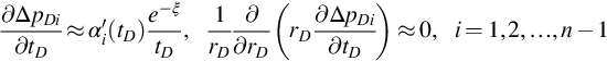 (B.17)
Using Eq. (3.10) as approximate pD, we have
∂pD∂tD≈e−ξ2tD
 (B.18)
Substituting Eq. (B.7) into Eq. (B.8a) and using Eqs. (B.17), (B.18), we get (after canceling e−ξtD)
Di[∑j=1n−1(1−wsj)α′ij−∑j=1i−1α′j]+α′iηDi+1−k˜Di−1wiαi−1+k˜Di(1wi+1wi+1)αi−k˜Di+1wi+1αi+1=−Di2,i=1,2,…,n−1
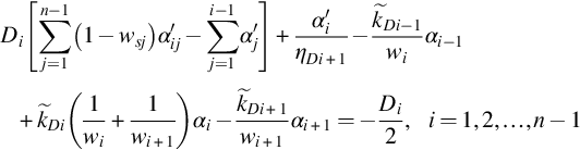 (B.19)
The initial conditions can be set as
αi(0)=0,i=1,2,…,n−1
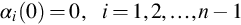 (B.20)
because the crossflow is zero at tD=0 .
.
Eq. (B.19) includes first-order differential equations with constant coefficients. The general solution is the sum of a particular solution and the general solution for the corresponding homogeneous equations. If we let α′j=0 , then Eq. (B.14) is obtained again to determine the particular solution, which is αsj. The corresponding homogeneous equations are
Di[∑j=1n−1(1−wsj)α′j−∑j=1i−1α′j]+α′iηDi+1−k˜Di−1wiαi−1+k˜Di(1wi+1wi+1)αi−k˜Di+1wi+1αi+1=0,i=1,2,…,n−1
 (B.21)
The solution of Eq. (B.21) has the form
αi(tD)=xie−λtD,i=1,2,…,n−1
 (B.22)
Substituting Eq. (B.22) into Eq. (B.21), we get
−Di[∑j=1n−1(1−wsj)λxj−∑j=1i−1λxj]−λxiηDi+1−k˜Di−1wixi−1+k˜Di(1wi+1wi+1)xi−k˜Di+1wi+1xi+1=0,i=1,2,…,n−1
 (B.23)
Let λj and Xj=(x1,j,x2,j,…,xn,j)T , and j=1,2,…,n−1
 be the eigenvalues and the corresponding eigenvectors of Eq. (B.23). The general solution of Eq. (B.19) is then
αi(tD)=αsi+∑j=1n−1ajxi,je−λjtD,i=1,2,…,n−1
 (B.24)
where aj are arbitrary constants determined by the boundary conditions (Eq. B.20)
αsi+∑j=1n−1ajxi,j=0,i=1,2,…,n−1
 (3.16)
The explicit theoretical results for two- and three-layer cases can be obtained readily with the above theory. For more than three layers, the solution is generally obtained numerically because of the eigenvalue problem (Eq. B.23).