Determination of Total Productivity by a Constant Wellbore Pressure Flow Test and the Crossflow Behavior in Multilayer Reservoirs
Abstract
The single-phase unsteady flow in a multilayer reservoir with crossflow when each layer produces under a constant wellbore pressure is studied. Approximate theoretical expressions for the total flow rate and the crossflows between layers are given and compared with numerical solutions. The crossflow behavior under constant wellbore pressures is discussed. A constant-pressure flow test can be used to determine the total (kh) value of the multilayer reservoir.
The max effective hole-diameter mathematical model describing flow of slightly compressible fluid through a two-layer reservoir with crossflow is solved rigorously. The model considers all layers are perforated that flows at a constant wellbore pressure. The effect of formation damage is included in the model. The new model is numerically stable when the skin is positive and negative. The effect of the reservoir parameters such as permeability, vertical permeability, skin, outer boundary conditions, and storativity on the layer production rate and total rate are investigated.
Keywords
Multilayer reservoir; Crossflow; Constant wellbore pressure; Interpretation method; Max effective hole-diameter mathematical model
5.1 Assumption and Approximate Theoretical Solution of the Problem
In 1949, Van Everdingen and Hurst (1949) gave the unsteady flow solutions for both the constant terminal rate case and the constant terminal pressure case when a well penetrates a homogeneous layer. Since then, the transient well test methods, based on the constant terminal rate solution, were studied deeply and used widely in practice. Paralleling to the constant-rate flow test method, Jacob and Lohman (1952) developed a method for analyzing the constant-pressure flow test in a single layer reservoir, which could be used to determine the (kh) value and skin factor. The constant-pressure flow test was described by Earlougher (1977), also, in his monograph. Unfortunately, this test method was seldom used in practice. The reason might be that it is much easier to measure wellbore pressure accurately than it is to measure flow rate accurately. However, constant-rate tests may inadvertently become constant-pressure tests, so we still need a method for analyzing such tests.
In Chapters 1 and 3, we have studied the constant total flow rate case when each layer is perforated in a two-layer reservoir or an arbitrary n-layer reservoir. We shall use the results obtained in Chapters 1 and 3.
In this chapter, we will examine the unsteady flow with crossflow in an n-layer reservoir when each layer produces under a constant wellbore pressure. Simple theoretical expressions for the asymptotic crossflow and the total flow rate are developed and compared with the numerical simulation results. It will be shown that these theoretical expressions agree very well with the numerical results. The simple expression for the total flow rate can be used to determine the total kh value of the reservoir.
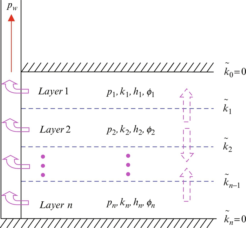
The following assumptions are used in this work: The n-layer reservoir is infinite and each layer is homogeneous; the reservoir is filled with a slightly compressible fluid; the semipermeable model can be used to approximate the actual reservoir; Gravity can be neglected. Suppose a well penetrates all the n layers, and each layer begins to produce under a constant wellbore pressure from time ![]() (see Fig. 5.1). The problem can be expressed as follows:
(see Fig. 5.1). The problem can be expressed as follows:
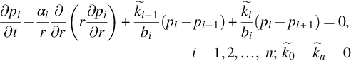
The boundary conditions are
The initial conditions are
where ![]() ,
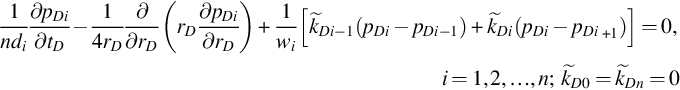
, ![]() , and c is compressibility. Using the following dimensionless expressions,
, and c is compressibility. Using the following dimensionless expressions,

and introducing the new variables:

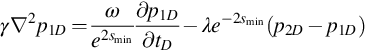
Eq. (5.1) becomes
An approximate analytical solution can be obtained as follows: the total rate qD diminishes with time when the well produces with a constant wellbore pressure for each layer. If the form of qD(tD) is known, the above problem can be replaced by a variable-rate flow problem.
Now we try to find the expression for qD(tD). From Chapter 3 we know that
is a good approximation of the kh-weighted pressure F when all the layers are perforated and produce with a constant total rate, where
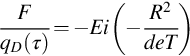
According to the superposition principle, function F can be approximated by
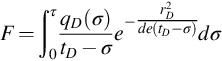
when the total rate qD changes with time. If qD(σ) is replaced by qD(tD) in Eq. (5.6), the integral value will decrease, since qD(tD) is a monotonically decreasing function. As a remedy, we can increase the integral interval. There exists a value T for each tD such that
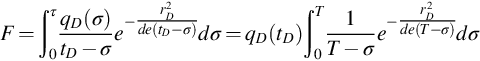
Using the transformation ![]() the above formula becomes
the above formula becomes

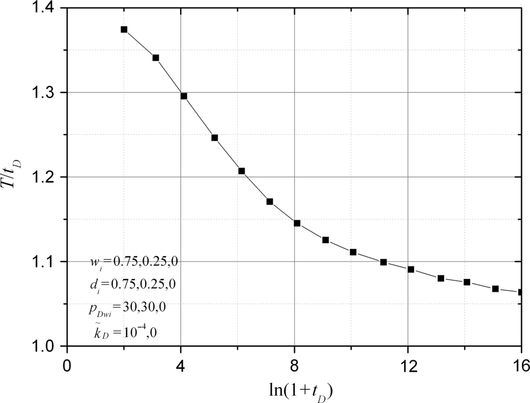
Here, T is a function of tD and needs to be determined. We can simply let ![]() . In this case, Eq. (5.7) is a good approximation of F. This might be useful in some cases, but a more reasonable choice of T is to allow the following:
. In this case, Eq. (5.7) is a good approximation of F. This might be useful in some cases, but a more reasonable choice of T is to allow the following:

The relationship of T and tD is shown in Fig. 5.2, which is obtained from numerical simulation for some cases. In practice it is better to calculate T from Eq. (5.8) directly, since constant wellbore pressures cannot be maintained strictly. From Eq. (5.7) we have
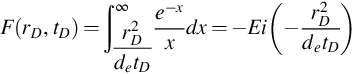
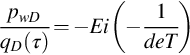
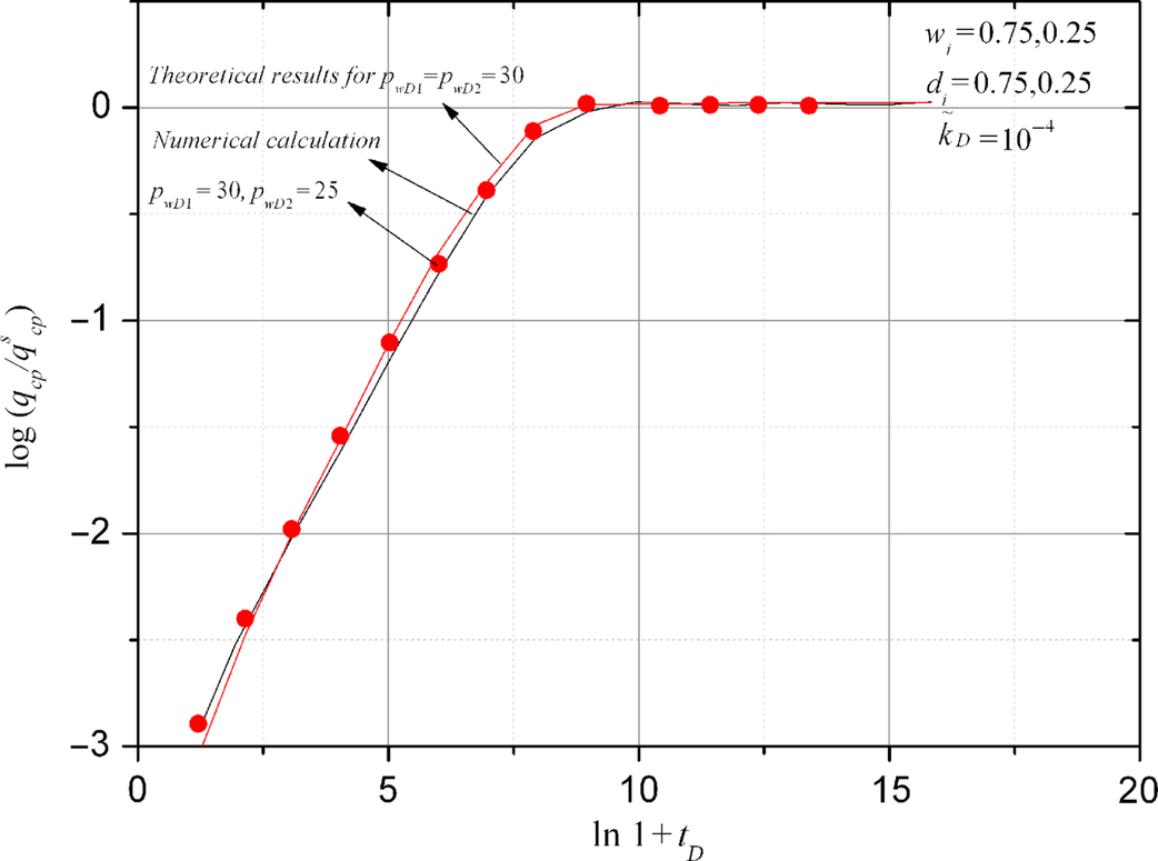
This formula agrees quite well with numerical results, as shown in Fig. 5.7. Using the boundary conditions in Eqs. (5.4)–(5.9), we get
where

Eq. (5.10) at times of interest reduces to
where ![]() is Euler's constant. When we express Eq. (5.12) in practical oilfield units of psi, B/D, cp, md, and ft, so it becomes
is Euler's constant. When we express Eq. (5.12) in practical oilfield units of psi, B/D, cp, md, and ft, so it becomes

where
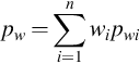
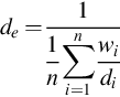
is the kh-weighted wellbore pressure and
is the effective diffusivity of the reservoir. B is the formation volume factor, and t′ is the dimension time corresponding to T.
Eq. (5.13) tells us that the total productivity of the multilayer reservoir can be determined by the slope of ![]() versus log(t′). This is quite similar to the drawdown test analysis. The only difference is that log(t′) is used instead of log(t).
versus log(t′). This is quite similar to the drawdown test analysis. The only difference is that log(t′) is used instead of log(t).
It is indicated in Chapter 1 that there are two kinds of crossflow in a homogeneous layered reservoir. One is caused by different boundary pressures and another is caused by different diffusivities for different layers. In the cases we study here, these two crossflows may exist if the constant wellbore pressures for different layers are different.
The crossflow caused only by different diffusivities when a well produces with a constant flow rate is studied in detail in Chapter 3. The theory and formulas can be used here if variables F and fi in Chapter 3 are replaced by ![]() and
and ![]() , the corresponding quantities per unit output rate. From Chapter 3 we have
, the corresponding quantities per unit output rate. From Chapter 3 we have


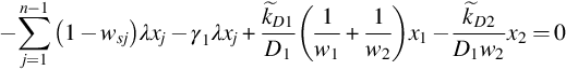
and λk, Xi,k, ![]() is the kth eigenvalue and corresponding eigensolution of the following equations:
is the kth eigenvalue and corresponding eigensolution of the following equations:


where
a0k, ![]() are determined by the following equations:
are determined by the following equations:
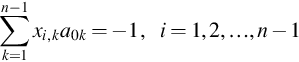
after xi,k is determined by Eq. (5.20). Based on numerical examples, all the eigenvalues are positive. The terms including ![]() in Eq. (5.17) will approach zero when tD is long, and ai(tD) will converge to the steady state solution asi.
in Eq. (5.17) will approach zero when tD is long, and ai(tD) will converge to the steady state solution asi.
We define the area crossflow as
and the area crossflow rate as
From Eq. (5.16) we have
where

qci has a maximum at ![]() . The peak value is
. The peak value is
where ![]() . When tD is long, ai converges to asi. Using Eq. (5.18), we get the steady peak value of qci
. When tD is long, ai converges to asi. Using Eq. (5.18), we get the steady peak value of qci
These formulas are exactly the same as those in Chapter 3.
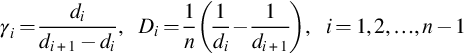
The crossflow caused by different boundary pressures develops with time and gradually converges to a steady state. The analysis solution for the steady pressure differences between layers is
and is given in the Appendix C. Here, ωi and dij, ![]() are the eigenvalues and eigensolutions of Eqs. (C.3), (C.4) respectively, and βi is determined by Eq. (5.30). K0 is the modified Bessel function.
are the eigenvalues and eigensolutions of Eqs. (C.3), (C.4) respectively, and βi is determined by Eq. (5.30). K0 is the modified Bessel function.
The total crossflow should be the sum of these two kinds of crossflow.
5.2 Numerical Results and Comparison with the Approximation Theory
In order to study the crossflow phenomenon and to test the above approximation theory, some two- and three-layer cases were calculated using a standard finite difference method. For convenience, a new pair of variables,
is used in the numerical calculation. Part of the calculation results will be shown below. All parameters are dimensionless.
5.2.1 Flow Rate of Each Layer Changes with Time
Fig. 5.3 shows how the flow rate of each layer changes with time in a two-layer reservoir. The flow rate diminishes very quickly at first and diminishes slower and slower when time increases. When the wellbore pressures for different layers are different, qDi/qD, the ratio of the rate for layer i to the total rate changes constantly with time. When the wellbore pressures are the same, qDi/qD changes with time when time is short and converges to the productivity ratio wi when time is long enough.

5.2.2 kh-Weighted Pressure Changes with Time
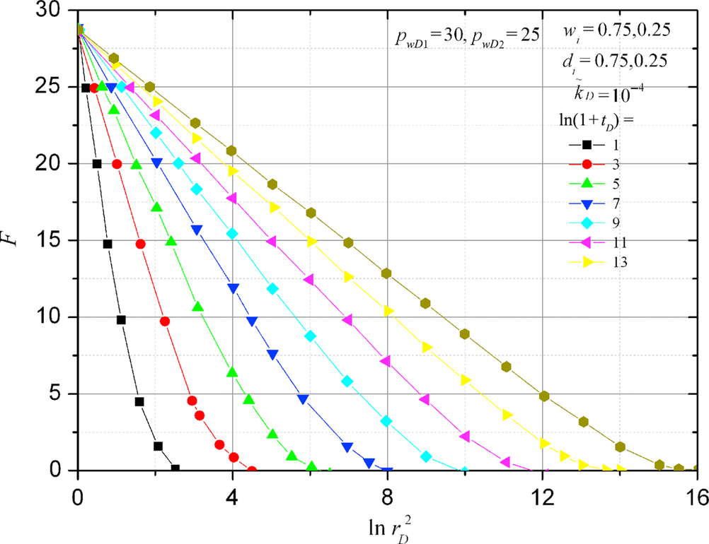
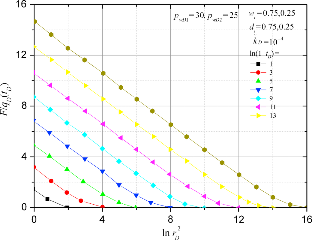
Figs. 5.4 and 5.5 show the distributions of kh-weighted pressure F and ![]() at a different time tD. It can be seen how the constant wellbore pressure problem is changed to a constant terminal rate problem when F/qD is used. Figs. 5.6 and 5.7 show that the numerical calculation of
at a different time tD. It can be seen how the constant wellbore pressure problem is changed to a constant terminal rate problem when F/qD is used. Figs. 5.6 and 5.7 show that the numerical calculation of ![]() agrees very well with the Ei function.
agrees very well with the Ei function.

 with time T. (After Gao (1983c) SPE 12581, Permission to publish by the SPE, Copyright SPE.)
 by the Ei function. (B) The approximation of by the Ei function. (After Gao (1983c) SPE 12581, Permission to publish by the SPE, Copyright SPE.)
5.2.3 Distributions of Pressure Difference Changes with Time
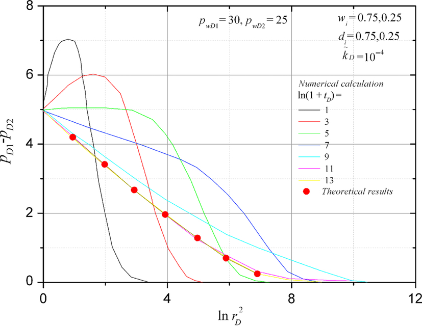
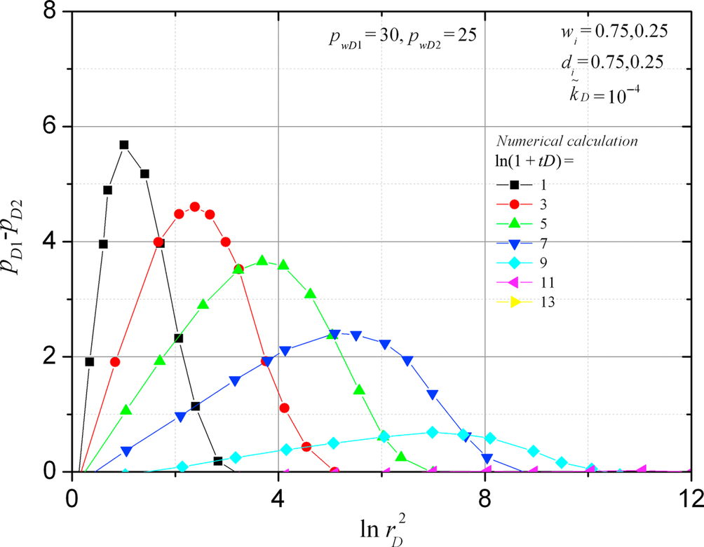
Figs. 5.8 and 5.9 show the distributions of pressure difference at different times for a two-layer reservoir when the constant wellbore pressures are different and the same, respectively. When the wellbore pressures are different, the pressure difference will gradually converge to a steady state. This steady state coincides with the theoretical solution. When wellbore pressures are the same, the pressure difference will go to zero with increasing time.
5.2.4 Distributions of Area Crossflow
Fig. 5.10 shows the distributions of area crossflow for a two-layer reservoir when wellbore pressures are different. The area crossflow develops from a single peak curve into a two-peak curve. The peak near well represents the crossflow caused by different wellbore pressures and becomes stable when time is long. When the wellbore pressures are the same, this peak will not appear. The peak away from the wellbore represents the crossflow caused by different diffusivities. The height of the second peak diminishes with time. From Fig. 5.10 we can see that the theory agrees quite well with numerical results.

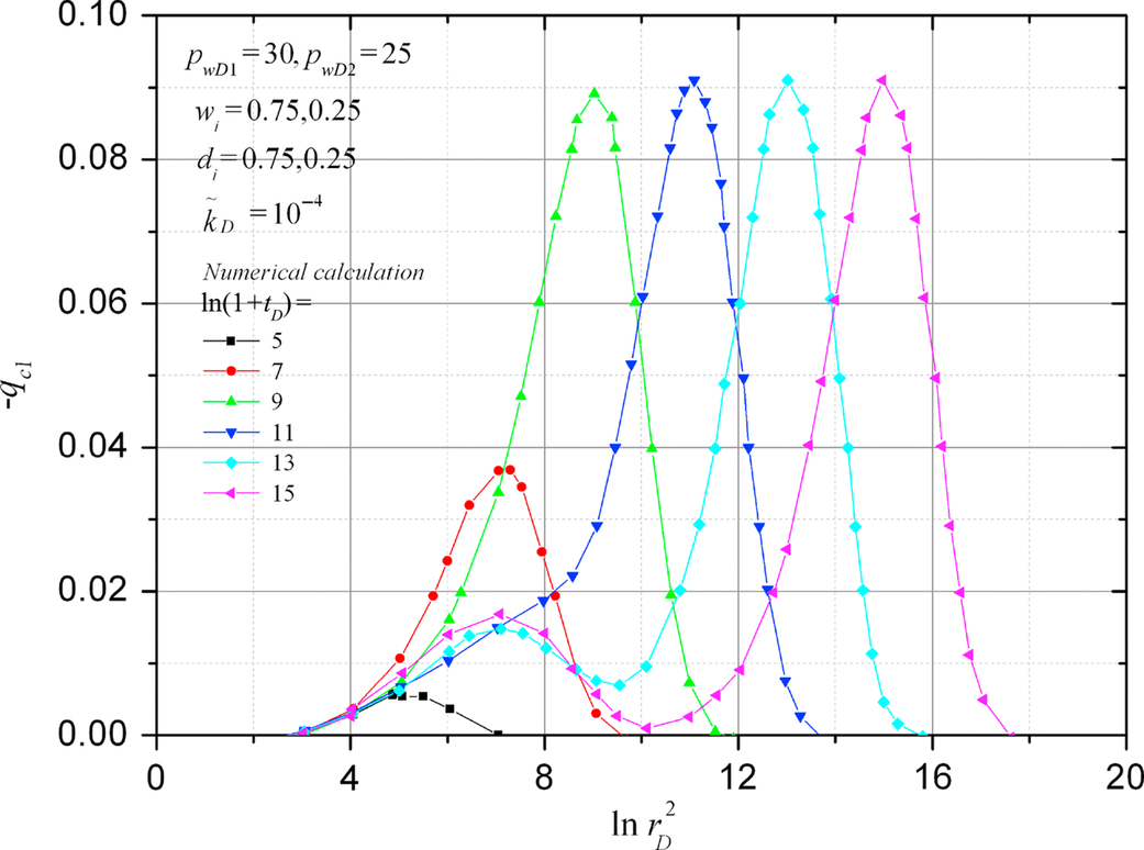
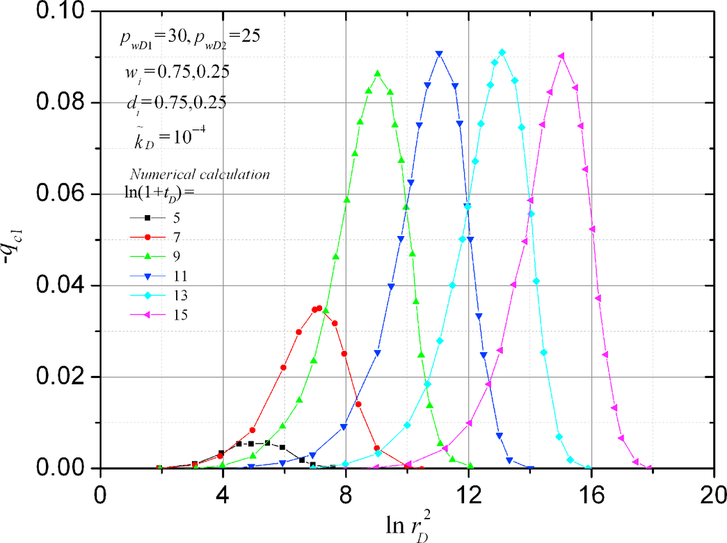
Figs. 5.11 and 5.12 show the distributions of the area crossflow rate qc1 for a two-layer reservoir when the wellbore pressures are different and the same, respectively. The distribution of qc1 will develop from a one-peak curve into a two-peak curve if the wellbore pressures are different. The first peak, which represents the crossflow caused by different boundary pressures, will increase with time. The second peak, which represents the crossflow caused by different diffusivities, moves forward like an unchanged wave when time is long. This phenomenon has been seen when the constant terminal rate flow was studied. Comparing Figs. 5.10–5.12 we can conclude that when time is long, the crossflow caused by different wellbore pressures is independent of the change of flow rate. The crossflow caused by different diffusivities is proportional to the total flow rate.
5.2.5 The Peak Value of qci Changes with Time
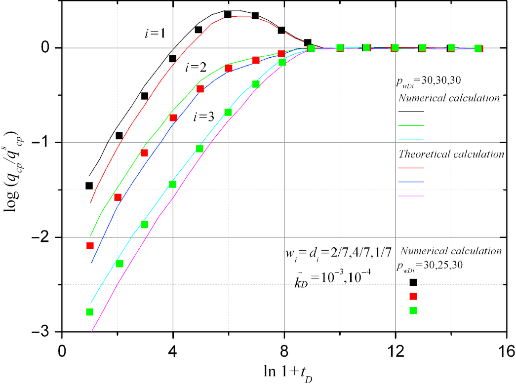
Figs. 5.13 and 5.14 show the change of the peak value of qci with time for a two-layer reservoir and a three-layer reservoir respectively. When time is short, ![]() is almost a straight line. When time is long, the peak value converges to a constant value. From these figures it can be seen that the theory agrees very well with the numerical results. When the wellbore pressure differences are not very large, the crossflow, caused by the wellbore pressures, has only a small influence on the peak value of the crossflow caused by different diffusivities. This is the reason why the theoretical curves agree very well with the cases when wellbore pressures are not that much different from each other.
is almost a straight line. When time is long, the peak value converges to a constant value. From these figures it can be seen that the theory agrees very well with the numerical results. When the wellbore pressure differences are not very large, the crossflow, caused by the wellbore pressures, has only a small influence on the peak value of the crossflow caused by different diffusivities. This is the reason why the theoretical curves agree very well with the cases when wellbore pressures are not that much different from each other.
5.3 Exact Solution of a Two-Layer Reservoir with Crossflow Under a Constant Pressure Condition
5.3.1 Model Description
The reservoir model for the two-layer system is shown in Fig. 2.1. We consider a two-layer reservoir that is enclosed at the top and bottom and at the outer radius by an impermeable boundary/constant pressure boundary or infinite boundary. The reservoir is homogeneous in the radial direction and heterogeneous in the vertical direction and is filled with a slightly compressible fluid of constant viscosity. The gravity effect is assumed to be negligible. The initial pressure is identical in both layers, and the well is produced at a constant pressure. Wellbore storage effects are not considered. In describing the formation crossflow between two adjacent layers, the semipermeable wall model is selected. Suppose a well penetrates two layers, each layer produces under a constant wellbore pressure.
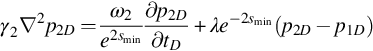
The dimensionless governing equation is
Initial condition:
Infinite outer boundary condition:
Constant pressure outer boundary condition:
No-flow outer boundary condition:

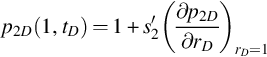
Wellbore boundary conditions:

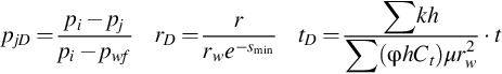
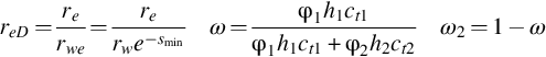
where

5.3.2 Derivation of Solutions for Pressure and Rate
Eqs. (5.31)–(5.38) are transformed into a Laplace domain with respect to tD:
The solutions for this system are the modified Bessel function K0 and I0. The dimensionless pressure can be written as follows:
where σj is the function of ωj, smin, γj and the Laplace space variable z. Substitution of Eq. (5.41) into Eqs. (5.39)–(5.40) results in the following:
For the system to have a nontrivial solution, the matrix must be zero. Two σ2 solutions are the following:
where

Once all the eigenvalues are found, the solution for the dimensionless pressure in layer j can be expressed as
According to Eqs. (5.42)–(5.43),
where,
According to outer boundary condition, the relationship of Ajk and Bjk is
For the infinite outer boundary condition, Eq. (5.34):
For the constant-pressure outer boundary condition, Eq. (5.35):
For the no-flow outer boundary condition, Eq. (5.36):

Dimensionless pressure in layer j can be expressed as
where
According to skin factor inner boundary condition,


Production rate of layer j is
5.3.3 Numerical Inversion of the Laplace Transform and Discussion of Results
Fig. 5.15 shows how the flow rate of each layer changes with time in a two-layer reservoir. The flow rate diminishes very quickly at first and diminishes slower and slower when time increases. When the wellbore pressures are the same, qjD/qD, the ratio of the rate for layer i to the total rate, changes with time when time is short and converges to the productivity ratio γ and γ2 when time is long enough.
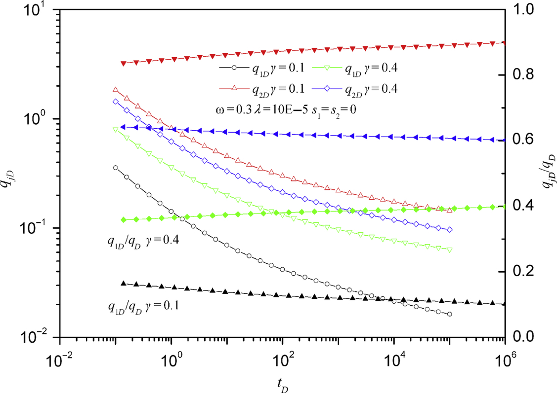
Fig. 5.16 shows how the qjD/qD changes with semipermeability. Three different regimes occur in a two-layer reservoir. At an early time, before crossflow is established, the response is the same as that for two-layer without crossflow. At a later time, qjD/qD converges to the productivity ratio γ and γ2. At an intermediate time, a transition behavior appears. For smaller vertical permeability, the transition occurs later.
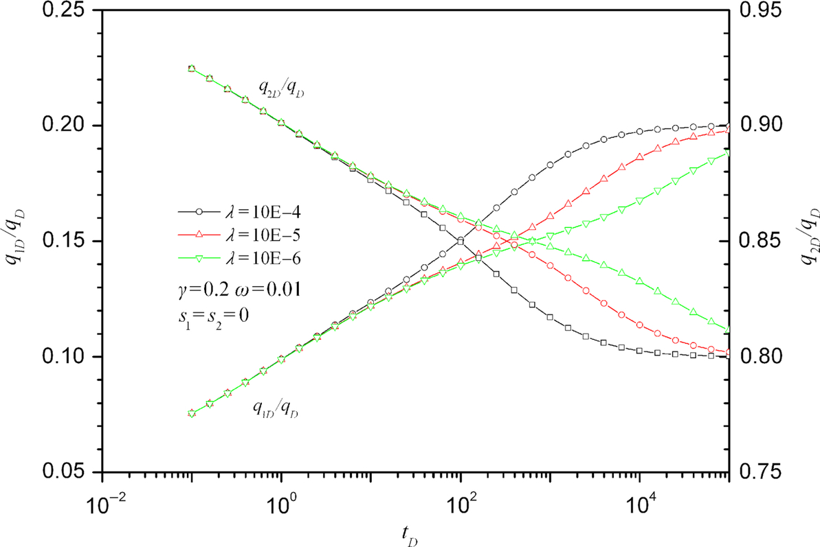
Fig. 5.17 shows how the qjD/qD changes with skin of Layer 1. qjD/qD converges to a constant when time is long enough. If ![]() , q1D/qD will converge to γ. If
, q1D/qD will converge to γ. If ![]() , q1D/qD doesn't converge to γ. We can find that if
, q1D/qD doesn't converge to γ. We can find that if ![]() , the constant of Layer 1 will be more than γ. If
, the constant of Layer 1 will be more than γ. If ![]() , the constant of Layer 1 will be less than γ.
, the constant of Layer 1 will be less than γ.

Fig. 5.18 shows how the flow rate of each layer changes with storativity. When the wellbore pressures are the same, qjD/qD, the ratio of the rate for Layer 1 to the total rate changes with time when time is short and converges to the productivity ratio γ and γ2 when time is long enough. For smaller storativity of Layer 1, the transition occurs early.

Fig. 5.19 shows how the flow rate of each layer changes with outer boundary conditions. qjD/qD, the ratio of the rate for Layer 1 to the total rate, converges to the productivity ratio γ and γ2 for infinite and constant-pressure outer boundary conditions. qjD/qD converges to a constant, but it is not equal to γ and γ2 for the no-flow boundary. For a smaller boundary, the effect occurs early.
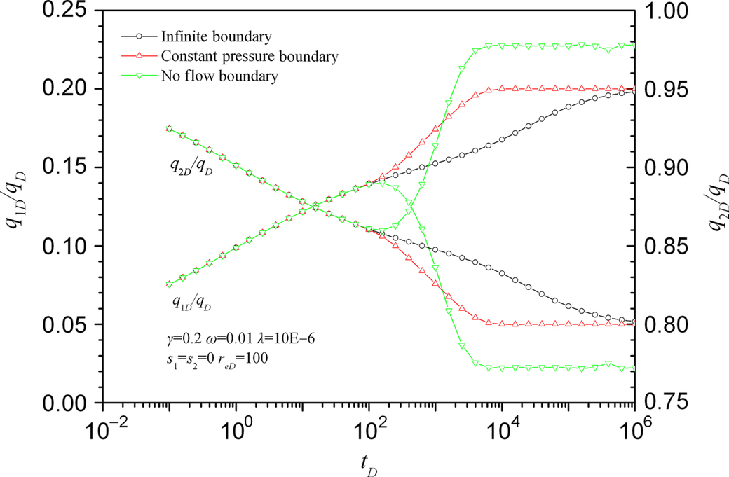
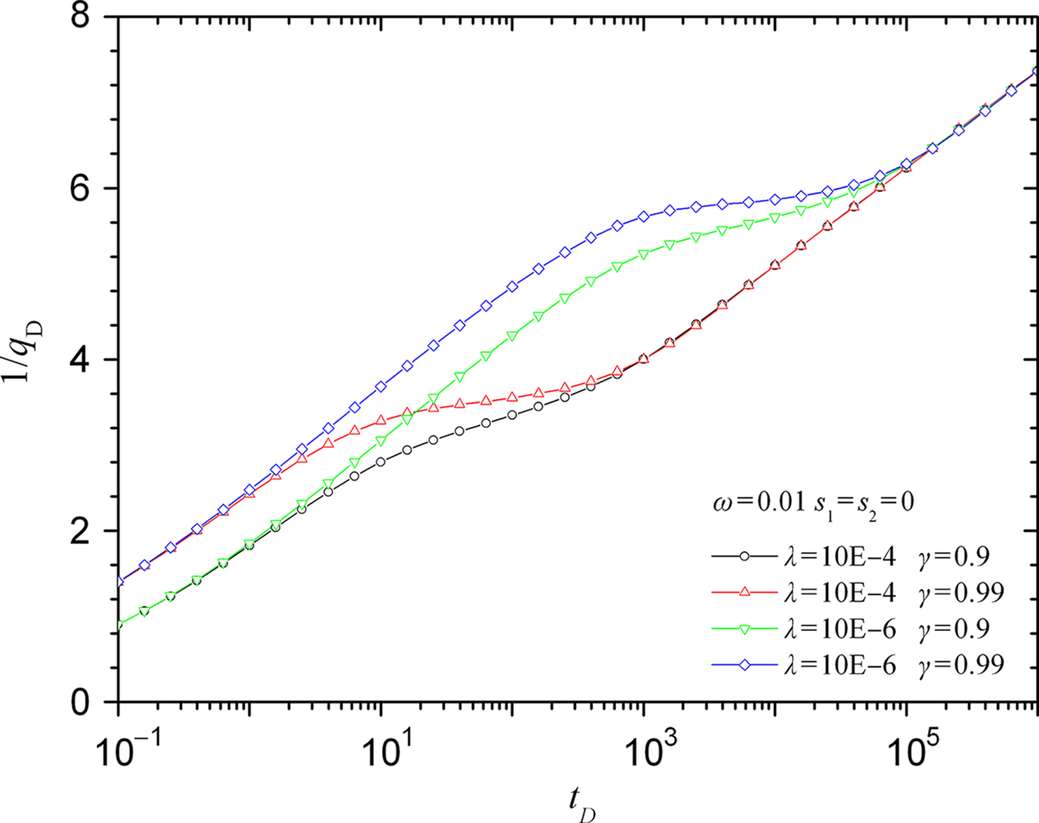
Fig. 5.20 shows how the 1/qD changes with time. Three different regimes occur in a two-layer reservoir. There are two lines. At early time, the smaller γ is, the 1/qD is. The smaller λ is, the later the transition occurs. At a later time, 1/qD of different parameters will converge to a line.
5.4 Summary
From what we have shown above, the following conclusions about the crossflow behavior can be drawn:
(1) The constant wellbore pressure problem can be replaced by a corresponding constant total flow rate problem if F/qD, the kh-weighted pressure per unit rate, and fi/qD, the pressure differences per unit rate, are used.
(2) The part of area crossflow rate, caused by different diffusivities, at first develops with time and then gradually reaches a quasisteady state. In the quasisteady state, it moves forward like an unchanged wave. Its behavior is described by the theory given in Chapter 3 for the case when all the layers are perforated and produce with a constant total rate.
(3) In the quasisteady state period, the pressure differences between layers and the crossflow caused by different wellbore pressures will reach a steady state and will not be influenced by the flow rate change.
(4) The ratio of the flow rate, qDi/qD, changes constantly when wellbore pressures are different for different layers, and it will converge to the productivity ratio wi when the wellbore pressures are the same.
(5) The total flow rate diminishes with time and can be expressed by Eqs. (5.10) or (5.12) when each layer produces under a constant wellbore pressure in a multilayer reservoir. The total productivity of the multilayer reservoir can be determined by the slope of ![]() versus log(t) curve at the straight line part.
versus log(t) curve at the straight line part.
(6) Three different regimes occur in a two-layer reservoir. At an early time, before crossflow is established, the response is the same as that for the two-layer reservoir without crossflow. At a later time, qjD/qD converges to a constant. At an intermediate time, a transition behavior appears. For smaller vertical permeability, the transition occurs later. If ![]() , q1D/qD will converge to γ. If
, q1D/qD will converge to γ. If ![]() , q1D/qD doesn't converge to γ. We can find that if
, q1D/qD doesn't converge to γ. We can find that if ![]() , the constant of Layer 1 will be more than γ. If
, the constant of Layer 1 will be more than γ. If ![]() , the constant of Layer 1 will be less than γ.
, the constant of Layer 1 will be less than γ.
(7) Curves of 1/qD with time have two lines; between two lines is an intermediate regime. The smaller the γ, the smaller 1/qD is. The smaller the λ, the later the transition occurs. At a later time, the 1/qD of different parameters will converge to a line.