1

Analysis of Nonhomogeneous Helical Systems Using Electrodynamical Methods

Models of helical systems are composed using surfaces with isotropical and anisotropical conductivity and magnetodielectric layers among them [1,2,3]. As a result of the solution of Maxwell’s equations, a dispersion equation can be derived. Using this equation, we can find the retardation factor and characteristic impedance versus frequency.

The electrodynamical method has been successfully applied for analysis of homogeneous helical systems by Vainoris, Kirvaitis, and Staras [1], Staras et al. [2], and Kirvaitis [3]. In this chapter, we will consider application of an electrodynamical method for analysis of nonhomogeneous systems. The chapter is based on Staras, Skudutis, and Kleiza [4], Kleiza and Staras [5], and Staras and Kleiza [6].

1.1  Modeling of Nonhomogeneous Helical Systems

Helical systems with round and rectangular cross sections are applied in practice. The view of a rectangular cross-section helical system is shown in Figure 1.1(a). Isotropically and anisotropically conducting planes (Figure 1.1b) are used in the models of helical systems with elongated rectangular cross sections when the system is homogeneous along the helix conductor [1,2,3].

Unfortunately, as a result of the solution of Maxwell’s equations, we learn that the amplitude of voltages and currents on the anisotropical planes modeling the plane parts of the elongated helix are not the same at shields asymmetrically located with respect to the helix (as in Figure 1.1a). Then the model does not correspond to the real helical system.

If the distance between the helix and its shields periodically changes along the helical conductor, the model presented in Figure 1.1(c) can be used. In this model, the anisotropic plane conducting in the direction of helical conductors is used to model the helix of the system, and the isotropically conducting surface is used to model the shield. Analysis based on the model [2] shows that periodical variation of the helix surroundings causes increase of retardation in the low-frequency range.

FIGURE 1.1
(a) The cross-section view of the helix containing and internal shield, and (b, c) models of a helical system. 1: Helical conductor; 2: internal shield; 3: anisotropically conducting plane characterizing helical conductors; 4: isotropic surface modeling shield.

We can take into account periodic variation of helix surroundings using the multiconductor line method. Staras et al. [2] have shown that the retardation factor of the helical system with asymmetrically located shields is given by

$k_{RLF}=\frac{2h}{L}\sqrt{1+\frac{1}{4}{\left(\sqrt{\frac{Y_1}{Y_2}-\sqrt{\frac{Y_2}{Y_1}}}\right)}^2.}$

(1.1)

Here, h is half of the length of the helix turn, L is the step of the helix, and Y₁ and Y₂ are characteristic admittances of helix conductors on the sides of the helix.

According to Equation (1.1), at Y₁ = Y₂, the retardation factor of the system is equal to the structural retardation k_Rs = 2h/L. At Y₁ ≠ Y₂, we obtain k_RLF > k_Rs.

The retardation factor in the low-frequency range increases with an increase of the ratio Y₁/Y₂. Thus, inhomogeneity of the slow-wave structure causes increase of retardation in the low-frequency range. Investigations of nonhomogeneous helical, meander, and other slow-wave structures confirm this idea [2,7,8].

To reveal the reasons for the effect, let us consider the periodic delay line consisting of segments of vacuumed coaxial lines with characteristic impedances Z_C1, Z_C2 and the same lengths of segments. In the frequency range where the period of the structure is considerably less than the wavelength, we can find equivalent capacitance and equivalent inductance using the following expressions:

$C_{1e}=\frac{C_{11}+C_{12}}{2},$

(1.2)

$L_{1e}=\frac{L_{11}+L_{12}}{2},$

(1.3)

where C₁₁, C₁₂, L₁₁, L₁₂ are capacitances and inductances of the segments of the line per unit of length.

Using Equations (1.2) and (1.3), we can easily derive an expression for delay time in the nonhomogeneous coaxial line:

$t_d=l\sqrt{L_{11}{C}_{11}}\sqrt{1+\frac{1}{4}{\left(\sqrt{\frac{C_{11}}{C_{12}}-\frac{C_{12}}{C_{11}}}\right)}^2},$

(1.4)

Here, l is the length of the line.

Expression (1.1) is similar to Expression (1.4). Taking this into account, we can consider the nonhomogeneous helical system as the system consisting of segments of homogeneous helical lines located along the helical conductor. Thus, we can find the equivalent capacitance and equivalent inductance per unit of length of the helical line using the following equations:

$C_{1e}=\frac{l_1{C}_{11}+l_2{C}_{12}}{l},$

(1.5)

$L_{1e}=\frac{l_1{L}_{11}+l_2{L}_{12}}{l},$

(1.6)

where

l = l₁ + l₂

l₁ and l₁ are the lengths of the periodic segments of the line

L₁₁ C₁₁ and L₁₂, C₁₂ are distributed parameters of the segments

Using the described idea, we can simplify modeling and analysis of nonhomogeneous helical systems with respect to the methods used by Staras et al. [2] and Vainoris, Staras, and Cuplinskas [7]. At known equivalent distributed parameters, retardation factor and characteristic impedance are given by [9]

$k_R=c_0\sqrt{L_{1e}{C}_{1e}},$

(1.7)

$Z_C=\sqrt{L_{1e}/C_{1e}},$

(1.8)

where c₀ is the electromagnetic wave velocity in free space (vacuum).

Using similar expressions for segments, we can find that

$L_{11}=\frac{k_{R1}{Z}_{C1}}{c_0},$

(1.9)

$L_{12}=\frac{k_{R2}{Z}_{C2}}{c_0},$

(1.10)

$C_{11}=\frac{k_{R1}}{Z_{C1}{C}_0},$

(1.11)

$C_{12}=\frac{k_{R2}}{Z_{C2}{C}_0},$

(1.12)

where k_R1, k_R2, Z_C1, and Z_C2 are retardation factors and characteristic impedances of homogeneous segments.

Substituting Equations (1.9),(1.10),(1.11),(1.12) into Equations (1.5,(1.6),(1.7),1.8), at l₁ = l₂, we obtain

$k_R=\frac{1}{2}(k_{R1}+k_{R2})\sqrt{1+\frac{k_{R1}{k}_{R2}}{{\left(k_{R1}+k_{R2}\right)}^2}{\left(\sqrt{\frac{Z_{C2}}{Z_{C1}}}-\sqrt{\frac{Z_{C1}}{Z_{C2}}}\right)}^2},$

(1.13)

$Z_C=\sqrt{Z_{C1}{Z}_{C2}}\sqrt{\frac{k_{R1}{Z}_{C1}+k_{R2}{Z}_{C2}}{k_{R1}{Z}_{C2}+k_{R2}{Z}_{C1}}}.$

(1.14)

A detailed analysis of homogeneous helical systems is presented in references 1–3 and other papers and monographs. General solutions of Maxwell’s equations and boundary conditions are used, and the set of algebraic equations is obtained. After eliminating amplitude coefficients, the dispersion equation and expression for the retardation factor are derived. Finally, using the solution of the dispersion equation and relationships between amplitude coefficients, characteristic impedance can be found.

Using the described method, based on calculation of equivalent distributed parameters, we can derive the expression for the retardation factor of the system consisting of a helix with an asymmetrically inserted internal shield:

$k_R=\cot \Psi \sqrt{1+\frac{1}{4}{\left(\sqrt{\frac{\sinh kc\cdot e^{-kc}}{\sinh kb\cdot e^{-kb}}}-\sqrt{\frac{\sinh kcb\cdot e^{-kb}}{\sinh kc\cdot e^{-kc}}}\right)}^2},$

(1.15)

where

ψ is the angle of helical conductors with respect to the cross-section plane of the system (cotψ = 2h/L)

b, c, and h are dimensions characterizing the cross section of the system (Figure 1.1a)

L is the helix step

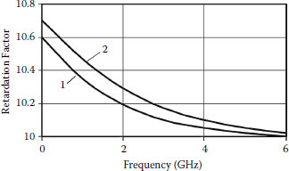
FIGURE 1.2
Retardation factor versus frequency at cot ψ = 10, c = 2b. 1: Using Equation (1.9); 2: according to references 2 and 6.

In the low-frequency range (at kb ≫ 1 and kc ≫ 1), we can simplify Equation (1.15):

$k_{RLF}=\cot \Psi \sqrt{1+\frac{1}{4}{\left(\sqrt{\frac{c}{b}}-\sqrt{\frac{b}{c}}\right)}^2}.$

(1.16)

Results of the calculation are presented in Figure 1.2. Curve 1 is plotted using Equation (1.15). Results of calculations [2,7] using the model presented in Figure 1.1(c) are represented by curve 2. Curves 1 and 2 are close to each other. The relative difference of ordinates is less than 1%–2%. Here it is important to notice that only a limited number of electromagnetic field harmonics is taken into account at calculations in Staras et al. [2] and Vainoris et al. [7].

We can find that at cot ψ = 10 and c = 2b, according to Equation (1.16), retardation factor k_{R LF} = 10.6. At low frequency, we can obtain the same value of retardation factor using Equation (1.1) at 2h/L = 10 and Y₁ = 2Y₂.

The presented information testifies that the developed method is suitable for analysis of nonhomogeneous systems. Further, we will use it for simulation of complex inhomogeneous helical systems.

1.2  Simulation of Axially Symmetrical Helical System

In addition to symmetrical helical systems that are systems with plane symmetry, systems with axial symmetry are possible. The cross-section view of a helical system with axial symmetry (Figure 1.3a) is similar to that with plane symmetry. On the other hand, winding directions of helices in the systems with plane symmetry are opposite. Analysis of helical systems with plane symmetry can be simplified using an electric wall in the symmetry plane. Winding directions of helices in the axially symmetrical helical systems are the same (Figure 1.3b), and we can easily find that, because of interaction of helices, axially symmetrical helical systems must be considered as nonhomogeneous systems.

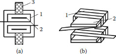
FIGURE 1.3
(a) The cross section of the axially symmetrical helical system and (b) a fragment of helical electrodes at removed external shield. 1: Helix; 2: internal shield; 3: dielectric holder.

Let us consider the axially symmetrical helical system using the described extension of the electrodynamical method. The fragment of the cross section of the axially symmetrical helical system is presented in Figure 1.4(a). An electrode of the system consists of four homogeneous sections along a helix turn. Models of these homogeneous sections are presented in Figure 1.4(b, c, d). They consist of anisotropically and isotropically conducting planes modeling helix and shields. The dielectric layer in Figure 1.4(d) models the dielectric holder of the helix.

FIGURE 1.4
(a) A fragment of the cross section of an axially symmetrical helical system and (b-d) models of homogeneous sections of a helical electrode. 1: Helix; 2: internal shield; 3: dielectric holder; 4: anisotropic planes modeling coupled parts of helices in the central section of the system; 5: isotropic plane modeling internal shield; 6: anisotropic plane modeling helix; 7: isotropic plane modeling external shield; 8: space filled by dielectric material modeling a dielectric holder.

Assuming the idea that characteristics of the nonhomogeneous system can be found at known characteristics of its homogeneous sections, we can rearrange Equations (1.5) and (1.6) to the more general form of

$C_{1e}=\frac{\Sigma l_i{C}_{1i}}{\Sigma l_i},$

(1.17)

$L_{1e}=\frac{\Sigma l_i{L}_{1i}}{\Sigma l_i},$

(1.18)

where l_i, L_1i, and C_1i are the length, inductance, and capacitance (per unit of length) of the ith section of the helical turn, respectively.

We can find characteristics of homogeneous sections of the system using methods developed in Vainoris et al. [1], Staras et al. [2], and Kirvaitis [3]. According to these authors, retardation factor k_R1 and characteristic impedance Z_C1 of the structure presented in Figure 1.4(b) are given by

$k_{R1}=\sqrt{\frac{\sinh k_{1}c\cdot \cosh k_{1}b}{\cosh k_{1}c\cdot \sinh k_{1}b}}\cot \Psi$

(1.19)

and

$Z_{C1}=\frac{1}{l_t}\sqrt{\frac{{\text{μ}}_{\text{0}}}{{\text{ε}}_{\text{0}}}}\frac{k_{L1}}{k_1}\frac{\sinh k_1(c-b)\cdot \sinh k_{1}b}{\sinh k_{1}c},$

(1.20)

where

b and c are dimensions of the cross section

l_t is the length of the helix turn

ψ is the angle of helix winding

k₁ = ω/v_ph is the wave number

ω is frequency

ν_ph is the phase velocity of the electromagnetic wave

ε₀ and μ₀ are dielectric permittivity and magnetic permeability

In the low-frequency range (at k₁c ≪ 1 and k₁(c − b) ≪ 1), we can use the simplified expressions for retardation factor and characteristic impedance:

$k_{R1LF}=\sqrt{\frac{c}{b}}\cot \Psi ,$

(1.21)

$Z_{C1LF}=\frac{1}{l_t}\sqrt{\frac{{\text{μ}}_{\text{0}}}{{\text{ε}}_{\text{0}}}(c-b)}\sqrt{\frac{b}{c}}\cot \Psi .$

(1.22)

In the high-frequency range (at k₁c ≫ 1 and k₁(c − b) ≫ 1),

$k_{R1HF}=\cot \Psi ,$

(1.23)

$Z_{C1HF}=\sqrt{\frac{{\text{μ}}_{\text{0}}/{\text{ε}}_{\text{0}}}{2\text{θ}}},$

(1.24)

where θ = ωt_t is the phase angle between voltages on neighbor turns and t_t = l_t/c₀ is the delay time of the electromagnetic wave propagating with velocity c₀ along a turn.

We can use the models of helices containing internal and external shields (Figure 1.4c, d) for modeling of the second and third sections of the axially symmetrical helical system. Then the retardation factor and characteristic impedance are given by [1]

$k_{Ri}=\sqrt{\frac{{\text{ε}}_{ri}\tanh k_i{d}_{i1}+\tanh k_i{d}_{i2}}{\tanh k_i{d}_{i1}+\tanh k_i{d}_{i2}}}\cot \Psi ,$

(1.25)

$Z_{Ci}=\frac{1}{l_t}\sqrt{\frac{{\text{μ}}_{\text{0}}}{{\text{ε}}_0}}\frac{k_{Ri}}{k_i}\frac{\tanh k_i{d}_{i2}\cdot \tanh k_i{d}_{i1}}{{\text{ε}}_{ri}\tanh k_i{d}_{i2}+\tanh k_i{d}_{i1}},$

(1.26)

where i is the number of the section.

In the low-frequency range,

$k_{RiLF}=\sqrt{\frac{{\text{ε}}_{ri}{d}_{i1}+d_{i2}}{d_{i1}+d_{i2}}}\cot \text{ψ,}$

(1.27)

$Z_{CiLF}=\frac{1}{l_t}\sqrt{\frac{{\text{μ}}_{\text{0}}}{{\text{ε}}_{\text{0}}}}{d}_{i1}{d}_{i2}\sqrt{\frac{d_{i1}+d_{i2}}{{\text{ε}}_{ri}{d}_{i1}+d_{i2}}}\cot \text{ψ}\text{.}$

(1.28)

At high frequencies,

$k_{RiHF}=\sqrt{{\text{ε}}_{re}}\cot \Psi ,$

(1.29)

$Z_{CiHF}=\frac{\sqrt{{\text{μ}}_{\text{0}}/{\text{ε}}_{\text{0}}{\text{ε}}_{re}}}{2\text{θ}},$

(1.30)

where ε_re = (1 + ε_r)/2.

At known characteristics of the sections, using Equations (1.9,(1.10),(1.11),1.12), (1.17), and (1.18), we can find the retardation factor and characteristic impedance of the axially symmetrical helical system:

$k_R=\frac{1}{l_t}\sqrt{{\displaystyle \sum _1^n{l}_j{k}_{Rj}{Z}_{\text{C}j}{\displaystyle \sum _1^n\frac{l_j{k}_{Rj}}{Z_{\text{C}j}}}}},$

(1.31)

$Z_C=\sqrt{\frac{{\displaystyle \sum _1^n{l}_j{k}_{Rj}{Z}_{\text{C}j}}}{{\displaystyle \sum _1^n{l}_j{k}_{Rj}/Z_{\text{C}j}}}},$

(1.32)

where n is number of sections (n = 4).

For calculations of the retardation factor and characteristic impedance of a homogeneous section, we can select the value of the wave number k¡, find the value of the retardation factor, and, finally, find values of frequency and characteristic impedance.

Using Equation (1.31), values of parameters at the same frequency are necessary. Then we recommend the following procedures of calculation.

We find values of the retardation factor and characteristic impedance in the low-frequency range using simplified expressions Equations 1.21 and (1.27). At higher frequency f, we calculate values of the retardation factor of sections using iterations [10]. We begin iterations from an approximate value of retardation factor k_Rx. Initially, we can take k_Rx = k_{Ri LF}. In the following steps (at higher frequency values), we can use the value of the retardation factor found in the previous step. When the value of retardation factor k_Rx at selected frequency f is determined, we can find the value of the wave number:

$k_x=\frac{\text{ω}}{{\upsilon }_{ph}}=\frac{2\text{π}f{k}_{Rx}}{c_0}=k_0{k}_{Rx}.$

(1.33)

At a known wave number value, we find the value of the retardation factor of the section using Equations (1.19) and (1.25). We can evaluate the precision of calculation using

$\Phi =k_{Li}(k_x)-\frac{c_0{k}_x}{2\text{π}f}.$

(1.34)

According to the developed algorithm, at Φ ≠ 0, we increase or decrease the value of the wave number (depending on the sign of the function Φ) and repeat calculation of the retardation factor. We continue iterations until the sign of function Φ becomes opposite. The value of the retardation factor in this step of iterations is considered as the value corresponding to the selected frequency.

FIGURE 1.5
(a) Retardation factor and (b) characteristic impedance of the axially symmetrical helical system versus frequency: 1: cotψ = 10, l_t, = 20, b = 1, c − b = 1, l₁ = 10, d_i1 = 1, d_i2 = 1, l₂ + l₃ + l₄ = 10 mm, ε_r3 =1; 2: ε_r3 = 6; 3: 2h/L = 10, x₄ = 20, w′₄ = 1, w₄ = 1, x₄ − x₃ = 10, w₁ = w₂ = w₃ = 1, w′₁ = w″₂ = w″₃ = 1, x₁ = 0, x₂ = x₃ = 10, p = 0.4, l = 0.8 mm, ε_r = ε′_r = ε″_r = 1; 4: ε_r = 1, ε′_r = 6, ε″_r = 3; 5: ε_r = 1, ε′_r = 6, ε″_r = 3.5. (According to Staras, S., and A. Gaivelis 1989. Communication Equipment Technique, Radio Measurement Technique. 7:73–77.)

Characteristics of the axially symmetrical helical system are presented in Figure 1.5. Curves 1 and 2 are obtained using the described extension of the electrodynamical method. Curves 3, 4, and 5 represent the results obtained using the multiconductor line method [11]. According to Figure 1.5, in the low-frequency range, results of calculations obtained using the electrodynamical method precisely coincide with results obtained using the multiconductor line method. Differences increase with frequency.

We can reveal reasons for methodical errors that appear at application of the electrodynamical method considering simplified expressions Equations 1.22 and (1.28) for characteristic impedances. Taking into account that the ratio l_t/cotψ at small angle ψ is approximately equal to the helix step, we can rearrange Equation (1.26) to

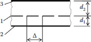
FIGURE 1.6
The fragment of longitudinal section of the helical system: 1: Helix; 2: internal shield; 3: external shield.

$Z_{CiLF}=\frac{1}{c_0({C^{\prime }}_1+{C^{\prime }}_2)},$

(1.35)

where C′₁₁ = ε₀Δ/d₁ and C′₁₂ = ε₀Δ/d₂ are capacitances of the multiconductor line (per unit of length) that appear due to internal and external shields (Figure 1.6).

Thus, results of calculations using the electrodynamical method correspond to helical systems containing infinitely thin helical conductors and small gaps between neighbor conductors (when the width of a conductor is close to the helix step Δ). As a result, the differences between results obtained using the mentioned methods in the high-frequency range are small when the thickness of helical conductors is at least two times less than the gap between conductors and the cross section is filled by a homogeneous dielectric. With a nonhomogeneous dielectric (curves 2, 4, and 5), the values of the retardation factor and characteristic impedance in the high-frequency range obtained using the multiconductor line method are dependent on dielectric permittivity of material in the space between neighbor conductors. Unfortunately, methods used in Staras and Gaivelis [11] for calculation of characteristic admittances cannot be used for thin conductors.

On the other hand, comparison of calculation results shows that relatively simple models and the electrodynamical method can be used for simulation of helical systems in order to reveal their general properties and to find ways to search for systems with better characteristics.

It is enough to consider only two sections corresponding to the flat parts of the helix in order to reveal the general properties of the axially symmetrical helical system.

Characteristics of systems with identical characteristics to sections 2,3, and 4 are presented in Figure 1.7 (at ε_ri = 1) and Figure 1.8 (at ε_ri = 6). The “1” curves are characteristics of the central section of the axially symmetrical helical system model shown in Figure 1.4(b). The “2” curves are characteristics of the last sections. The characteristics of the axially symmetrical systems are presented by the “3” curves.

FIGURE 1.7
(a) Retardation factor and (b) characteristic impedance of the axially symmetrical helical system versus frequency at cotψ = 10, l_t = 20, b = 1, c − b = 1, l₁ = 10, d_i1 = 1, d_i2 = 1, l₂ + l₃ + l₄ = 10 mm, ε_r = 1. 1: Central section; 2: other sections; 3: characteristics of the system.

We see that dispersion of retardation is the characteristic feature of the axially symmetrical helical system filled by homogeneous dielectric. At low frequency, the retardation factor is greater than structural retardation (k_R > k_Rs = cotψ). The retardation factor decreases with frequency and approaches k_Rs in the high-frequency range. We can explain this effect, taking into account that distributed parameters periodically change along the helical conductors; additionally, at opposite polarities of input voltage, currents in the central part of the axially symmetrical system flow in the same directions, and coupling of electromagnetic fields is followed by increase of distributed inductances of helical electrodes. If frequency increases, the coupling decreases because of the surface character of the electromagnetic field in the slow-wave structure. As a result of this, the retardation factor decreases with frequency.

At ε_ri = 1, we can reduce the coupling of fields and dispersion of retardation, increasing the distance 2b between interacting helices. Unfortunately, this way is not acceptable in the case of traveling wave-deflecting systems because an increase of distance between the deflecting electrodes is followed by decreased sensitivity.

FIGURE 1.8
(a) Retardation factor and (b) characteristic impedance of the axially symmetrical helical system versus frequency at cotθ = 10, l_t, = 20, b = 0.5, c − b = 0.5, l₁ = 10, d_i1 = 0.4, d_i2 = 1, l₂ + l₃ + l₄ = 10 mm, ε_r = 6. 1: Central section; 2: other sections; 3: characteristics of the system.

According to Figure 1.8(a), dielectric holders tend to increase retardation with frequency. Then, as a result of opposite changes of retardation in the sections, we can reduce dispersion of retardation in the wide-frequency range (curve 3 in Figure 1.9a) considerably. Characteristics presented in Figure 1.9(a) obtained for the system containing four sections confirm this idea: At properly selected dimensions and materials, the retardation factor is practically constant in the wide-frequency range. Unfortunately, compensation of dispersion is followed by a more rapid fall of characteristic impedance with increase of frequency.

Thus, the relatively simple method based on the electrodynamical method and usage of mean distributed parameters can be applied for simulation of axially symmetrical and other complex helical systems.

Variation of distributed parameters along the helical conductor and coupling of helices in the middle section of the axially symmetrical system cause an increase of the retardation factor of the system in the low-frequency range. Characteristic impedance of the system decreases with frequency as in other helical systems.

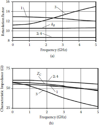
FIGURE 1.9
(a) Retardation factor and (b) characteristic impedance of the axially symmetrical helical system versus frequency at cotψ = 8.5, l_t = 16, l₁ = 6, l₂ = l₄ = 4, l₃ = 1.2 mm. 1: b = 0.3, c − b = 0.4; 2 and 4: d₂₁ = d₄₁ = 0.4, d₂₂ = d₂₂ = d₄₂ = 1; 3: d₃₂ = 3 mm, ε_r3 = 7.

Dielectric holders can help to increase retardation with frequency and to avoid dispersion of retardation. Further, let us apply the developed method for simulation of other complex nonhomogeneous helical systems.

1.3  Simulation of Complex Helical Systems without Internal Shields

In this section we will apply the developed method for analysis of helical systems without internal shields. Afterward, we will compose the generalized model for simulation of the systems containing nonhomogeneous dielectrics and isotropic and anisotropic shields.

1.3.1  Modeling and Properties of the Helix Asymmetrically Mounted inside the External Shield

Properties of systems having elongated rectangular cross sections and containing helices (without internal shields) symmetrically mounted with respect to external shields are considered in references 1 and 2, as well as in other papers. At the same time, it is important that, sometimes, we want to know properties of helices asymmetrically mounted inside external shields (helices with asymmetrical external shields). Models and analysis of this type of helical system are more complicated because symmetry conditions cannot be used for analysis of their models.

Let us consider the helical system with cross section shown in Figure 1.10(a). Models corresponding to the left and right sides of the system are presented in Figure 1.10(b) and (c). Taking into account that electromagnetic fields inside the helix practically do not depend on the distance between the helix and its shield, we can assume that, at propagation of the electromagnetic wave along the helical conductor on the left side of the system, conditions are similar to those in the model presented in Figure 1.10(b) and that, at propagation on the right side, conditions are similar to those in Figure 1.10(c). Thus, the model presented in Figure 1.10(b) can be used for calculation of distributed parameters for the left side, and the model presented in Figure 1.10(c) can be applied for calculation of distributed parameters for the right side [12,13,14,15].

Models of homogeneous helical systems in the absence of internal shields (as in Figure 1.10b, c) are examined in references 1 and 2. Capacitances and inductances per unit of length are given by

$C_1=2{\text{ε}}_{\text{0}}kh\frac{\cosh kd}{\cosh kb}\cdot \frac{1}{\sinh k(d-b{)}^{\prime }}$

(1.36)

$L_1=\frac{1}{2h}\cdot \frac{{\text{μ}}_{\text{0}}{\cot }^2\text{ψ}}{k}\cdot \frac{\sinh kb}{\sinh kd}\sinh k(d-b),$

(1.37)

FIGURE 1.10
(a) The view of the cross section of the asymmetrically shielded helix and models of its (b) left and (c) right sides. 1: Helix; 2: external shield; ψ: angle of winding.

where

h is the length of a half of a helix turn

ε₀, μ₀ are electric and magnetic constants, respectively

k = ω/c = 2π/λ is the wave number

Thus, we can use the same expressions for distributed parameters considering models (Figure 1.10b, c). For calculation of distributed parameters for the left and right sides, we must assume that d = d₁, k = k₁ and d = d₂, k = k₂, correspondingly. Afterward, we can use Equations (1.17) and (1.18) for calculation of equivalent parameters of the system.

Using the described extension of the electrodynamical method, we can derive expressions for the retardation factor and characteristic impedance of the helix with an asymmetrical external shield:

$k_R=c_0\sqrt{L_e{C}_e}=\frac{\cot \text{ψ}}{2}\sqrt{(A_1+A_2)(B_1+B_2)},$

(1.38)

$Z_C=\sqrt{\frac{L_e}{C_e}}=\frac{{\text{ρ}}_{\text{TEM}}\text{cot}\text{ψ}}{2h}\sqrt{\frac{B_1+B_2}{A_1+A_2},}$

(1.39)

where

$\begin{array}{c}{A}_i=k_i\frac{\cosh k_i{d}_i}{\cosh k_i{d}_i\cdot \sinh k_i{c}_i},\\ B_i=\frac{1}{k_i}\frac{\sinh k_{i}b\cdot \sinh k_i{c}_i}{\sinh k_i{d}_i},\end{array}$

i is the number of the side (i = 1; 2)

c₀ is the velocity of the electromagnetic wave in the free space

${\text{ρ}}_{\text{TEM}}=\sqrt{{\text{μ}}_0/{\text{ε}}_0}$ is the characteristic impedance of the free space

ψ is the angle of helix winding

c₁ = d₁ − b; c₂ = d₂ − b.

In the low-frequency range (at kb ≪ 1, kd₁ ≪ 1, and kd₂ ≪ 1),

$k_R{}_{LF}=\frac{\cot \text{ψ}}{2}\sqrt{b\left(\frac{c_1}{d_1}+\frac{c_2}{d_2}\right)\left(\frac{1}{c_1}+\frac{1}{c_2}\right)},$

(1.40)

$Z_{CLF}=\frac{{\text{ρ}}_{\text{TEM}}\cot \text{ψ}}{2h}\sqrt{b\frac{c_1/d_1+c_2/d_2}{1/c_1+1/c_2}}\cdot$

(1.41)

At d₁ = d₂ = d, the helical system is homogeneous and the expressions for retardation factor and characteristic impedance can be simplified to the known form [1,2]:

$k_R=\cot \text{ψ}\sqrt{\frac{\sinh kb\cdot \cosh kd}{\cosh kb\cdot \sinh kd}},$

(1.42)

$Z_C=\frac{1}{2h}\frac{{\text{ρ}}_{\text{TEM}}\cot \text{ψ}}{k_{R}k}\frac{\sinh kb}{\sinh kc}\sinh k(d-b).$

(1.43)

Characteristics of helices mounted inside external shields calculated using Equations (1.38) and (1.39) are presented in Figure 1.11. The “1” curves in Figure 1.11(a) and (b) are obtained at a constant distance of the external shield from the helix along the helical conductor (c₁ = c₂ in Figure 1.10a). They coincide with characteristics presented in references 1 and 2. According to these references, at a constant distance of the external shield, the retardation factor in the low-frequency range is less than the structural retardation. It increases with frequency and approaches the structural retardation at high frequencies.

FIGURE 1.11
(a) Retardation factor and (b) characteristic impedance versus frequency of the helix mounted in the external shield at cotψ = 10; h/b = 10; c₂/b = 0.25. 1: c₁/b = 0.25; 2: 0.6; 3: 3; 4: 5.5; 5: 16.6.

Generally, the retardation factor in the low-frequency range is dependent on conditions for electromagnetic waves on the left and right sides of the helix. With an increase of the ratio c₁/c₂ (inhomogeneity of the system along the helix conductor), the retardation factor in the low-frequency range increases (curves 4 and 5 in Figure 1.11a) and can exceed the structural retardation. Using this feature of the system, we can reduce dispersion of retardation considerably (curve 3 in Figure 1.11a). Characteristic impedance of the system decreases with frequency and is dependent on the distance of the shield from the helix. If this distance decreases, characteristic impedance also decreases and becomes less dependent on frequency (Figure 1.11b).

Figure 1.12(a) and (b) illustrates how the retardation factor and characteristic impedance in the low-frequency range depend on inhomogeneity of the system consisting of the helix asymmetrically mounted inside the external shield. According to Figure 1.12(a), by decreasing the gap between the external shield and the helix on one side of the helix, we can considerably (practically to 1.5 times) increase the retardation factor in the low-frequency range.

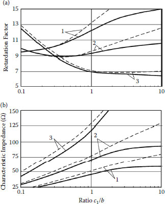
FIGURE 1.12
Characteristics illustrating how the (a) retardation factor and (b) characteristic impedance in the low-frequency range depend on the ratio c₁/b (inhomogeneity of the system consisting of the helix asymmetrically mounted inside the external shield) at cotψ = 10; h/b = 10. 1: c₂/b = 0.1; 2: 0.25; 3: 0.9.

The dashed lines in Figure 1.12(a) and (b) are obtained using the multiconductor line method. At c₁ / c₂ < 5, results obtained using the electrodynamical method are close to results obtained using the multiconductor line method. Differences between calculated values of characteristic impedance exist because we cannot take into account real dimensions of helical conductors using the electrodynamical method. On the other hand, the characteristics presented in Figure 1.12 testify that the developed simple extension of the electrodynamical method based on calculation of equivalent parameters can be successfully applied for simulation of helical systems without internal shields.

Let us further compose the generalized model of helical systems without internal shields.

1.3.2  Generalized Model of Helical Systems without Internal Shields

Many types of helical systems are used in practice. The systems can contain isotropic and anisotropic shields, dielectric holders, and layers of magnetodielectric materials.

Two types of asymmetrical helical systems containing dielectric holders are presented in Figure 1.13(a) and (b). An isotropic external shield is used in the system in Figure 1.13(a). The system in Figure 1.13(b) contains the external shield that can be considered anisotropic.

FIGURE 1.13
Helices with (a) isotropic, (b) anisotropic external shields, and models of (c) left and (d) right sides of the helical systems. 1: Helix; 2: external isotropic shield; 3: external anisotropic shield; 4: dielectric holder; 5: anisotropic planes modeling the helix; 6: isotropically conducting plane modeling the external shield; 7: anisotropically conducting (in the direction of the longitudinal axis of the system) plane modeling the anisotropical external shield; ε_r1 and ε_r2 are relative dielectric permittivities of dielectric material in the space inside and outside the helix.

Models of sections of the systems (Figure 1.13a, b) are shown in Figure 1.13(c) and (d). The structure shown in Figure 1.13(c) models the left sides of helical systems, and the structure in Figure 1.13(d) models the right sides. The structures presented in Figure 1.13(c, d) are models of the homogeneous helical systems investigated in references 1 and 3.

The retardation factor and characteristic impedance of helical systems modeled by the structure shown in Figure 1.13(c) are given by

$k_{R1}=\cot \text{ψ}\sqrt{\left({\text{ε}}_{r1}\frac{\sinh kb}{\cosh kb}+\frac{\cosh k{c}_1}{\sinh k{c}_1}\right)}\cdot \sqrt{\frac{\sinh k{c}_1\sinh kb}{\sinh k{d}_1}},$

(1.44)

and

$Z_{C1}=\frac{k_{R1}\cdot {\text{ρ}}_{\text{TEM}}}{2hk}\cdot \frac{\tanh k{c}_1}{{\text{ε}}_{r1}\tanh kb\tanh k{c}_1+1},$

(1.45)

where c₁ = d₁ − b is the distance of the shield from the helix on its left side.

The retardation factor and characteristic impedance of helical systems modeled by the structure shown in Figure 1.13(d) are given by

$k_{R2}=\cot \text{ψ}\sqrt{\frac{\left({\text{ε}}_{r2}\cosh kb\cosh k{c}_2+{\text{ε}}_{r1}\sinh kb\sinh k{c}_2\right)}{\sinh k{c}_2\cosh kb\sinh k(b+c_2+c_3)}\sinh kb\sinh k(c_2+c_3)}$

(1.46)

and

$Z_{C2}=\frac{k_{R2}\cdot {\text{ρ}}_{\text{TEM}}}{2hk}\frac{\tanh k{c}_2}{{\text{ε}}_{r1}\tanh kb\tanh k{c}_2+{\text{ε}}_{r2}},$

(1.47)

where c₂ = d₂ − b, c₃ = d₃ − b are dimensions of the right sides of helical systems (Figure 1.13a, b).

Using Equations (1.44),(1.45),(1.46),1.47) and Equations (1.2)–(1.3), we can derive expressions for calculation of characteristics of the helical systems that are under consideration [14]:

$\begin{array}{r}{k}_R=\frac{\cot \text{ψ}}{2}\sqrt{\frac{\sinh k_{1}b\sinh k_1{c}_1}{k_1\sinh k_1{c}_1}+\frac{\sinh k_{2}b\sinh k_2(c_2+c_3)}{k_2\sinh k_2(b+c_2+c_3)}}\\ \times \sqrt{k_1\frac{{\text{ε}}_{r1}\tanh k_{1}b\tanh k_1{c}_1+1}{\tanh k_1{c}_1}+k_2\frac{{\text{ε}}_{r1}\tanh k_{2}b\tanh k_2{c}_2+{\text{ε}}_{r2}}{\tanh k_2{c}_2}};\end{array}$

(1.48)

$Z_C=\frac{{\text{ρ}}_{\text{TEM}}\cdot k_R}{2h\left(k_1\frac{{\text{ε}}_{r1}\tanh k_{1}b\tanh k_1{c}_1+1}{\tanh k_1{c}_1}+k_2\frac{{\text{ε}}_{r1}\tanh k_{2}b\tanh k_2{c}_2+{\text{ε}}_{r2}}{\tanh k_2{c}_2}\right)}$

(1.49)

where k₁ and k₂ are the wave numbers in the structures modeling the left and right sides of the helical systems, respectively.

In the low-frequency range, we can use simplified expressions:

$k_{RLF}=\frac{\cot \text{ψ}}{2}\sqrt{b\left(\frac{c_1}{d_1}+\frac{c_2+c_3}{d_2+d_3}\right)\left(\frac{1}{c_1}+\frac{{\text{ε}}_{r2}}{c_2}\right)},$

(1.50)

$Z_{CLF}=\frac{{\text{ρ}}_{\text{TEM}}\cdot k_{RLF}}{2h}\cdot \frac{c_1{c}_2}{c_2+{\text{ε}}_{r2}{c}_1}.$

(1.51)

Using Equations (1.48,(1.49),(1.50),1.51), we can simulate many types of helical systems containing helices without internal shields. At d₂ and d₃, we obtain the system with an isotropic external shield. At d₁ = d₂ = d₃ ≫ b, Expressions (1.48)–(1.51) are mathematical models of the system containing an external anisotropic shield. Assuming d₁ = d₂ = d₃ and ε_r1 = ε_r2 = 1, we obtain the homogeneous system, and the expression for the retardation factor and characteristic impedance can be simplified to Equations (1.42) and (1.43).

Using Equations (1.48) and (1.49), we must know values of wave number k₁ and k₂ at the same frequency f. We can solve the problem using iterations (as in Section 1.2).

Using Equation (1.33), we can find the frequency corresponding to the selected value of wave number and found value of the retardation factor:

$f_i=\frac{c_0{k}_i}{2\text{π}{k}_{Ri}},$

(1.52)

where i (i = 1, 2) denotes the side of the helix and model (Figure 1.13c, d).

According to the developed algorithm, we select the value of wave number k₁ and, using Equations (1.46) and (1.52), find values of retardation factor k_R1 and frequency f₁. Then we change the wave number k₂ step by step and calculate retardation factor k_R2 and frequency f₂ until the condition

$\left|\frac{2(f_1-f_2)}{f_1+f_2}\right|\le \text{δ}$

(1.53)

is satisfied; here, δ is the maximal allowed relative error.

The determined values of wave numbers k₁, k₂ and the corresponding values of the retardation factor are used for calculation of the retardation factor and characteristic impedance of the system at a selected frequency using Equations (1.48) and (1.49).

The calculated characteristics are presented in Figure 1.14. The “1” curves are plotted for the helix symmetrically mounted in the external shield and are the same as the “1” curves in Figure 1.11. The “2” curves represent characteristics of the helical system containing an anisotropic external shield. We see that application of the anisotropic shield is followed by a considerable increase of the retardation factor, characteristic impedance in the low-frequency range, and considerable increase of retardation dispersion. The “3” curves illustrate the influence of the solid dielectric onto properties of the helical systems. An increase of dielectric permittivity of the medium in the space between the helix and the external shield causes an increase of retardation and decrease of characteristic impedance.

FIGURE 1.14
(a) Retardation factor and (b) characteristic impedance of the helical systems shown in Figure 1.13(a) (“1” curves) and Figure 1.13(b) (curves 2, 3, and 4) at cotψ = 10, h/b = 6.6. 1: c₁/b = c₂/b = 0.25, ε_r2 = 1; 2: c₁/b = c₂/b = 0.25, ε_r2 = 1; 3: c₁/b = c₂/b = 0.25, ε_r2 = 2; 4: c₁/b = 0.25, c₂/b = 5.6, ε_r2 = 1.

It is important that, using the anisotropic asymmetrically located shield, we can ensure small retardation dispersion at relatively high characteristic impedance (the “4” curves in Figure 1.14a, b).

For application of helical systems for deflection of electron beams in traveling-wave cathode-ray tubes, the distance between helical deflecting electrodes increases along the system from approximately 1 mm at the input to some millimeters at the output in order to have a greater useful area on the screen. Characteristic impedance of the system must be constant along the system. In order to compensate for the increase of characteristic impedance, shields are set at less distance with respect to helices. The developed method allows solving the problem of the design of traveling-wave deflecting systems.

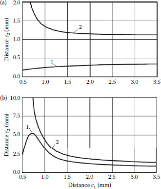
FIGURE 1.15
Characteristics illustrating how distance c₂ must change at changing distance c₁ in order to have (a) constant retardation factor k_R = 10 and (b) constant characteristic impedance Z_C = 100 Ω along the helical system at cotψ = 10, h/b = 10.1: isotropic external shield; 2: anisotropic external shield.

Characteristics in Figure 1.15(a) show how the distance c₂ between the helix and isotropic shield (curve 1) and between the helix and anisotropic shield (curve 2) must change in order to ensure a constant retardation factor at increasing distance c₁ between the helix and the shield. Similarly, characteristics in Figure 1.15(b) show how the distance c₂ between the helix and isotropic shield (curve 1) and between the helix and anisotropic shield (curve 2) must change in order to ensure constant characteristic impedance (Z_C = 100 Ω) at increasing distance c₁.

We see that it is not easy to design a system with a constant retardation factor and characteristic impedance. On the other hand, using characteristics presented in Figure 1.15, we can find the distance c₂ that allows us to ensure minimal variations of characteristics along the system.

Thus, the extension of the electrodynamical method based on equivalent parameters can be applied for simulation of helical systems without internal shields and allows solving important practical problems.

1.4  Summary

We developed the extension of the electrodynamical method for simulation of nonhomogeneous helical systems. The extension is based on calculation of equivalent distributed parameters for the existence of inhomogeneities along the helical conductor.

We proposed the model of the axially symmetrical helical system, derived expressions for calculation of frequency characteristics of the system, and revealed inherent features of axially symmetrical helical systems. These features can be taken into account at design phases of systems having a constant retardation factor in the wide-frequency range.

We proposed the generalized model for simulation of inhomogeneous systems containing helices (without internal shields), external isotropic or anisotropic shields, and dielectric holders or magnetodielectric layers in the cross section. The model can be applied for analysis of asymmetrical helical systems and symmetrical helical systems with plane symmetry. The presented results of calculations revealed inherent properties of the class of helical systems that do not contain internal shields. Using specific properties of the systems, we can reduce retardation dispersion considerably in the wide-frequency range.

The developed extension of the electrodynamical method can be applied for simulation and design of complex helical systems.

References

1.  Vainoris, Z., Kirvaitis, R., and Staras, S. 1986. Electrodynamic delay and deflection systems. Vilnius, Lithuania: Mokslas, 266. [In Russian.]

2.  Staras, S. et al. 1993. Super-wide band tracts of the traveling-wave cathode-ray tubes. Vilnius, Lithuania: Technika, 360. [In Russian.]

3.  Kirvaitis, R. 1994. Electrodynamic delay lines. Vilnius, Lithuania: Technika, 216. [In Lithuanian.]

4.  Staras, S., Skudutis, J., and Kleiza, A. 1997. Investigation of inhomogeneous helical systems using electrodynamical method. Electronics and Electrical Engineering 1 (10): 12–13. [In Lithuanian.]

5.  Kleiza, A., and Staras, S. 1997. Analysis of the axially symmetrical helical system using electrodynamical method. Eletronika’97, Conference Proceedings. Book 2. May 14–16, 1997, 45–46. [In Lithuanian.]

6.  Staras, S., and Kleiza, A. 1997. Analysis of the axially symmetrical helical system using electrodynamical method. Electronics and Electrical Engineering 4 (13): 30–34. [In Lithuanian.]

7.  Vainoris, Z., Staras, S., and Cuplinskas, A. 1988. Electrodynamical analysis of retardation in helical system containing asymmetrical shields. Communication Equipment Technique, Radio Measurement Technique 8:8–35. [In Russian.]

8.  Martavicius, R. 1996. Electrodynamic plain retard systems for wide-band electronic devices. Vilnius, Lithuania: Technika, 264. [In Lithuanian.]

9.  Vainoris, Z. 2004. Fundamentals of wave electronics. Vilnius, Lithuania: Technika, 513. [In Lithuanian.]

10.  Kleiza, A. 2000. Investigation of non-homogeneous electrodynamic systems. Doctoral dissertation, Vilnius Gediminas Technical University, Vilnius, Lithuania, 139. [In Lithuanian.]

11.  Staras, S., and Gaivelis, A. 1989. Analysis of axially symmetrical helical system with complicated cross section. Communication Equipment Technique, Radio Measurement Technique 7:73–77. [In Russian.]

12.  Staras, S., Skudutis, J., and Daskevicius, V. 1998. Investigation of helix asymmetrically mounted inside external shield. Electronics and Electrical Engineering 1 (4): 35–36. [In Lithuanian.]

13.  Skudutis, J., and Daskevicius, V. 1998. Generalized model of a helix with external shields. Elektronika’98, Conference Proceedings, Kaunas, May 19–20, 1998, 82–85. [In Lithuanian.]

14.  Skudutis, J. 2000. Theory and design of electrodynamic retard and deflecting systems. Summary of the research report presented for habilitation. Vilnius Gediminas Technical University, Vilnius, Lithuania, 36. [In Lithuanian.]

15.  Daskevicius, V. 2000. Investigation and design of helical delay line. Doctoral dissertation, Vilnius Gediminas Technical University, Vilnius, Lithuania, 91. [In Lithuanian.]