
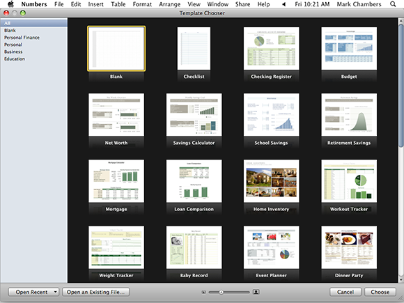
Figure 18-1: Hey, these templates aren’t frightening at all!
Chapter 18
Creating Spreadsheets with Numbers
In This Chapter
![]() Opening, saving, and creating spreadsheets
Opening, saving, and creating spreadsheets
![]() Selecting cells, entering data, and editing data
Selecting cells, entering data, and editing data
![]() Formatting cells
Formatting cells
![]() Adding and removing rows and columns
Adding and removing rows and columns
![]() Creating simple calculations
Creating simple calculations
![]() Adding charts to your spreadsheets
Adding charts to your spreadsheets
![]() Printing a Numbers spreadsheet
Printing a Numbers spreadsheet
Are you downright afraid of spreadsheets? Does the idea of building a budget with charts and all sorts of fancy graphics send you running for the safety of the hall closet? Well, good iMac owner, Apple has once again taken something that everyone else considers super-complex and turned it into something that normal human beings can use! (Much as Apple did with video editing, songwriting, and website creation — heck, is there any type of software that Apple designers can’t make intuitive and easy to use?)
In this chapter, I get to demonstrate how Numbers can help you organize data, analyze important financial decisions, and yes, even maintain a household budget! You’ll soon see why the Numbers spreadsheet program is specifically designed with the home Mac owner in mind.
Before You Launch Numbers . . .
Just in case you’re not familiar with applications like Numbers and Microsoft Excel — and the documents they create — let me provide you with a little background information.
A spreadsheet organizes and calculates numbers by using a grid system of rows and columns. The intersection of each row and column is a cell, and cells can hold either text or numeric values (along with calculations that are usually linked to the contents of surrounding cells).
Spreadsheets are wonderful tools for making decisions and comparisons because they let you “plug in” different numbers — such as interest rates or your monthly insurance premium — and instantly see the results. Some of my favorite spreadsheets that I use regularly include
![]() Car and mortgage loan comparisons
Car and mortgage loan comparisons
![]() A college planner
A college planner
![]() My household budget (not that we pay any attention to it)
My household budget (not that we pay any attention to it)
Creating a New Numbers Document
As does Pages, Apple’s desktop publishing application, Numbers ships with a selection of templates that you can modify quickly to create a new spreadsheet. (For example, after a few modifications, you can easily use the Budget, Loan Comparison, and Mortgage templates to create your own spreadsheets.)
To create a spreadsheet project file, follow these steps:
1. Click the Launchpad icon in the Dock.
2. Click the Numbers icon.
Numbers displays the Template Chooser window you see in Figure 18-1.
3. Click the type of document you want to create in the list to the left.
The document thumbnails on the right are updated with templates that match your choice.
4. Click the template that most closely matches your needs.
5. Click Choose to open a new document using the template you selected.
Opening an Existing Spreadsheet File
If a Numbers document appears in a Finder window (or you locate it using Spotlight or All My Files), you can just double-click the Document icon to open it; Numbers automatically loads and displays the spreadsheet. However, it’s equally easy to open a Numbers document from within the program. Follow these steps:
1. Double-click the Numbers icon to run the program.
2. Press ![]() +O to display the Open dialog.
+O to display the Open dialog.
3. Click the desired drive in the Devices list at the left of the dialog and then click folders and subfolders until you’ve located the desired Numbers document.
 If you’re unsure of where the document is, click in the Search box at the top of the Open dialog and type in a portion of the document name, or even a word or two of text it contains.
4. Double-click the spreadsheet to load it.
If you want to open a spreadsheet you’ve been working on over the last few days, click File ⇒Open Recent to display Numbers documents that you’ve worked with recently.
Save Those Spreadsheets!
Thanks to Lion’s Auto Save feature, you no longer have to fear losing a significant chunk of work because of a power failure or a coworker’s mistake. However, if you’re not a huge fan of retyping data, period, you can always save your spreadsheets manually after making a major change . Follow these steps to save your spreadsheet to your hard drive:
1. Press ![]() +S.
+S.
If you’re saving a document that hasn’t yet been saved, the Save As sheet appears.
2. Type a filename for your new spreadsheet.
3. Click the Where pop-up menu and choose a location to save the file.
This allows you to select common locations, such as your Desktop, Documents folder, or Home folder.
If the location you want isn’t listed in the Where pop-up menu, you can also click the down-arrow button next to the Save As text box to display the full Save As dialog. Click the desired drive in the Devices list at the left of the dialog and then click folders and subfolders until you reach the desired location. Alternatively, type the folder name in the Spotlight search box at the top right and double-click the desired folder in the list of matching names. (As an extra bonus, you can also create a new folder in the full Save As dialog.)
4. Click Save.
After you’ve saved the file the first time, you can use the Save a Version and Revert to Saved items on the File menu to save a “snapshot” of your Numbers document, or revert the document to a past version.
Exploring the Numbers Window
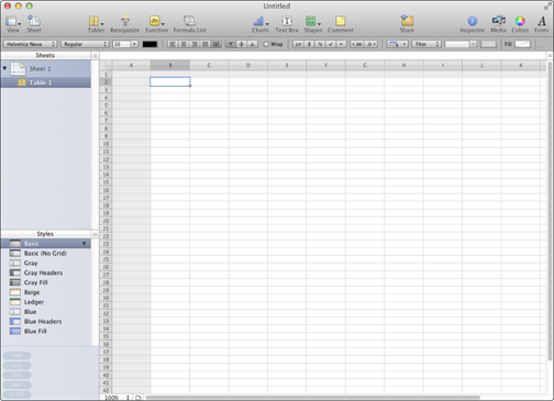
Apple has done a great job of minimizing the complexity of the Numbers window. Figure 18-2 illustrates these major points of interest:
![]() Sheets list: Because a Numbers project can contain multiple spreadsheets, they’re displayed in the Sheets list at the left of the window. To switch among spreadsheets in a project, click the top-level headings (each of which has a spreadsheet icon).
Sheets list: Because a Numbers project can contain multiple spreadsheets, they’re displayed in the Sheets list at the left of the window. To switch among spreadsheets in a project, click the top-level headings (each of which has a spreadsheet icon).
![]() Sheet canvas: Numbers displays the rows and columns of your spreadsheet in this section of the window; you enter and edit cell values within the sheet canvas.
Sheet canvas: Numbers displays the rows and columns of your spreadsheet in this section of the window; you enter and edit cell values within the sheet canvas.
![]() Toolbar: The Numbers toolbar keeps the most common commands you’ll use within easy reach.
Toolbar: The Numbers toolbar keeps the most common commands you’ll use within easy reach.
![]() Formula Box: You’ll use the Formula Box to enter formulas into a cell, allowing Numbers to automatically perform calculations based on the contents of other cells.
Formula Box: You’ll use the Formula Box to enter formulas into a cell, allowing Numbers to automatically perform calculations based on the contents of other cells.
![]() Format Bar: Located directly under the toolbar, the Format Bar displays editing controls for the object that’s currently selected. (If you enter an equal sign into the Formula Box, the Format Bar changes into the Formula Bar. No, I’m not making this up.) My goodness, this is starting to sound like that classic movie about the chocolate tycoon and those kids!
Format Bar: Located directly under the toolbar, the Format Bar displays editing controls for the object that’s currently selected. (If you enter an equal sign into the Formula Box, the Format Bar changes into the Formula Bar. No, I’m not making this up.) My goodness, this is starting to sound like that classic movie about the chocolate tycoon and those kids!
Figure 18-2: The Numbers window struts its stuff.
Navigating and Selecting Cells in a Spreadsheet
You can use the scroll bars to move around in your spreadsheet, but when you enter data into cells, moving your fingers from the keyboard is a hassle. For this reason, Numbers has various movement shortcut keys that you can use to navigate, and I list them in Table 18-1. After you commit these keys to memory, your productivity level shoots straight to the top.
Table 18-1 Movement Shortcut Keys in Numbers
|
Key or Key Combination |
Where the Cursor Moves |
|
Left arrow (←) |
One cell to the left |
|
Right arrow (→) |
One cell to the right |
|
Up arrow ( |
One cell up |
|
Down arrow ( |
One cell down |
|
Home |
To the beginning of the active worksheet |
|
End |
To the end of the active worksheet |
|
Page Down |
Down one screen |
|
Page Up |
Up one screen |
|
Return |
One cell down (also works within a selection) |
|
Tab |
One cell to the right (also works within a selection) |
|
Shift+Enter |
One cell up (also works within a selection) |
|
Shift+Tab |
One cell to the left (also works within a selection) |
You can use the mouse to select cells in a spreadsheet:
![]() To select a single cell, click it.
To select a single cell, click it.
![]() To select a range of multiple adjacent cells, click a cell at any corner of the range you want and then drag the mouse in the direction you want.
To select a range of multiple adjacent cells, click a cell at any corner of the range you want and then drag the mouse in the direction you want.
![]() To select a column of cells, click the alphabetic heading button at the top of the column.
To select a column of cells, click the alphabetic heading button at the top of the column.
![]() To select a row of cells, click the numeric heading button on the far left side of the row.
To select a row of cells, click the numeric heading button on the far left side of the row.
Entering and Editing Data in a Spreadsheet
After you navigate to the cell in which you want to enter data, you’re ready to type your data. Follow these steps to enter That Important Stuff:
1. Either click the cell or press the spacebar.
A cursor appears, indicating that the cell is ready to hold any data you type.
2. Type in your data.
 Spreadsheets can use both numbers and text within a cell; either type of information is considered data in the Spreadsheet World.
3. To edit data, click within the cell that contains the data to select it and then click the cell again to display the insertion cursor. Drag the insertion cursor across the characters to highlight them and then type the replacement data.
4. To simply delete characters, highlight the characters and press Delete.
5. When you’re ready to move on, press Return (to save the data and move one cell down) or press Tab (to save the data and move one cell to the right).
Selecting the Correct Number Format
After your data has been entered into a cell, row, or column, you still might need to format it before it appears correctly. Numbers gives you a healthy selection of formatting possibilities. Number formatting determines how a cell displays a number, such as a dollar amount, a percentage, or a date.
Characters and formatting rules, such as decimal places, commas, and dollar and percentage notation, are included in number formatting. So if your spreadsheet contains units of currency, such as dollars, format it as such. Then all you need to do is type the numbers, and the currency formatting is applied automatically.
To specify a number format, follow these steps:
1. Select the cells, rows, or columns you want to format.
2. Click the Inspector toolbar button.
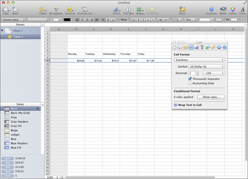
3. Click the Cells Inspector button in the Inspector toolbar to display the settings you see in Figure 18-3.
4. Click the Cell Format pop-up menu and click the type of formatting you want to apply.
Figure 18-3: From the Inspector, you can format the data you’ve entered.
Aligning Cell Text Just So
You can also change the alignment of text in the selected cells. (The default alignment for text is flush left and for numeric data, flush right.) Follow these steps:
1. Select the cells, rows, or columns you want to format.
See “Navigating and Selecting Cells in a Spreadsheet,” earlier in this chapter, for tips on selecting stuff.
2. Click the Inspector toolbar button.
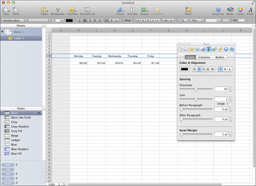
3. Click the Text Inspector button in the Inspector toolbar to display the settings you see in Figure 18-4.
4. Click the corresponding alignment button to choose the type of formatting you want to apply.
You can choose left, right, center, justified, and text left and numbers right. Text can also be aligned at the top, center, or bottom of a cell.
You can also select the cells you want to align and click the appropriate alignment button in the Format Bar.
Figure 18-4: Using the Inspector to change text alignment within a cell.
Do you need to set apart the contents of some cells? For example, you might need to create text headings for some columns and rows or to highlight the totals in a spreadsheet. To change the formatting of the data displayed within selected cells, select the cells, rows, or columns you want to format and then click the Font Family, Font Size, or Font Color buttons on the Format Bar.
Formatting with Shading
Shading the contents of a cell, row, or column is helpful when your spreadsheet contains subtotals or logical divisions. Follow these steps to shade cells, rows, or columns:
1. Select the cells, rows, or columns you want to format.
2. Click the Inspector toolbar button.
3. Click the Graphic Inspector button in the Inspector toolbar.
Numbers displays the settings you see in Figure 18-5.
4. Click the Fill pop-up menu to select a shading option.
5. Click the color box to select a color for your shading.
Numbers displays a color picker (also shown in Figure 18-5).
Figure 18-5: Adding shading and colors to cells, rows, and columns is easy in Numbers.

6. Click to select a color.
7. After you achieve the effect you want, click the Close button in the color picker.
8. Click the Inspector’s Close button to return to your spreadsheet.
The Fill function is also available on the Format Bar.
Inserting and Deleting Rows and Columns
What’s that? You forgot to add a row and now you’re three pages into your data entry? No problem. You can easily add or delete rows and columns. First, select the row or column that you want to delete or that you want to insert a row or column next to, and do one of the following:
![]() For a row: Right-click and choose Add Row Above, Add Row Below, or Delete Row from the shortcut menu that appears.
For a row: Right-click and choose Add Row Above, Add Row Below, or Delete Row from the shortcut menu that appears.
![]() For a column: Right-click and choose Add Columns Before, Add Columns After, or Delete Column from the shortcut menu that appears.
For a column: Right-click and choose Add Columns Before, Add Columns After, or Delete Column from the shortcut menu that appears.
If you select multiple rows or columns and choose Add, Numbers inserts the same number of new rows or columns as what you originally selected.
You can also insert rows and columns using the Table menu.
The Formula Is Your Friend
Sorry, but it’s time to talk about formulas. These equations calculate values based on the contents of cells you specify in your spreadsheet. For example, if you designate cell A1 (the cell in column A at row 1) to hold your yearly salary and cell B1 to hold the number 12, you can divide the contents of cell A1 by cell B1 (to calculate your monthly salary) by typing this formula into any other cell:
=A1/B1
By the way, formulas in Numbers always start with an equal sign (=).
“So what’s the big deal, Mark? Why not use a calculator?” Sure, but maybe you want to calculate your weekly salary. Rather than grab a pencil and paper, you can simply change the contents of cell B1 to 52, and — boom! — the spreadsheet is updated to display your weekly salary.
That’s a simple example, of course, but it demonstrates the basis of using formulas (and the reason that spreadsheets are often used to predict trends and forecast budgets). It’s the “what if?” tool of choice for everyone who works with numeric data.
To add a simple formula within your spreadsheet, follow these steps:
1. Select the cell that will hold the result of your calculation.
2. Click inside the Formula Box and type = (the equal sign).
The Formula Box appears to the right of the Sheets heading, directly under the Button bar. Note that the Format Bar changes to show a set of formula controls (a.k.a. the Formula Bar).
3. Click the Function Browser button, which bears the fx label.
(It appears next to the red Cancel button on the Formula Bar.)
4. In the window that appears, as shown in Figure 18-6, click the desired formula and click Insert to add it to the Formula Box.
Figure 18-6: If you have to use formulas, at least Numbers can enter them for you.

5. Click an argument button in the formula and click the cell that contains the corresponding data.
Numbers automatically adds the cell you indicated to the formula. Repeat this for each argument in the formula. (In case you’re not familiar with the term argument, it refers to a value specified in a cell that’s used by a formula. For example, the SUM formula adds the contents of each cell you specify together to produce a total; each of those cell values is an argument.)
6. After you finish, click the Accept button to add the formula to the cell.
That’s it! Your formula is now ready to work behind the scenes, doing math for you so that the correct numbers appear in the cell you specified.
To display all the formulas that you’ve added to a sheet, click the Formula List button in the toolbar.
Adding Visual Punch with a Chart
Sometimes you just have to see something to believe it — hence the ability to use the data you add to a spreadsheet to generate a professional-looking chart! Follow these steps to create a chart:
1. Select the adjacent cells you want to chart by dragging the mouse.
To choose individual cells that aren’t adjacent, you can hold down the ![]() key as you click.
key as you click.
2. Click the Charts button on the Numbers toolbar.
The Charts button bears the symbol of a bar graph.
Numbers displays the thumbnail menu you see in Figure 18-7.
3. Click the thumbnail for the chart type you want.
Numbers inserts the chart as an object within your spreadsheet so that you can move the chart. You can drag using the handles that appear on the outside of the object box to resize your chart. Figure 18-8 illustrates the 3-D chart I generated with just a couple of mouse clicks.
Click the Inspector toolbar button and you can switch to the Chart Inspector dialog, where you can change the colors and add (or remove) the chart title and legend.
4. To change the default title, click the title box once to select it; click it again to edit the text.
After you’ve added your chart to the sheet, you’ll note that it appears in the Sheets list, as also shown in Figure 18-8. To edit the chart at any time, just click the corresponding entry in the Sheets list.
Figure 18-7: Numbers displays the range of chart styles you can use.

Figure 18-8: My finished chart looks like someone with talent drew it for me!

..................Content has been hidden....................
You can't read the all page of ebook, please click here login for view all page.