Chapter 9 Moiré Metrology

The French word moiré originates from a type of textile, traditionally of silk, with a grained or watered appearance. Now moiré is generally used for a fringe that is created by superposition of two (or more) patterns such as dot arrays and grid lines (see Figure 9.1).

Moiré phenomenon can be observed in our everyday surroundings, like the folded netting. Some moiré patterns need to be got rid of as an undesired artifact, for example, the patterns produced during scanning a halftone picture. Some moiré patterns, on the contrary, act as very useful phenomena for different application fields. For instance, in the textile industry, designers intentionally generate beautiful moiré patterns with silk fabrics; in health-care field, the moiré is applied to diagnostic test of scoliosis, which is more common in teenage females.

In this chapter, applications of the moiré phenomenon to the optical metrology are described. In moiré metrology, the moiré fringe is resulted from the superposition of two periodic gratings structured with 1D lines. One of these gratings is called reference grating, and the other one is object grating, which is to be distorted by a structure whose deformation or shape is represented by the resulting moiré fringes. The moiré fringe created by these two superposed gratings in the same plane is termed in-plane moiré and by two gratings in different planes is out-of-plane moiré.

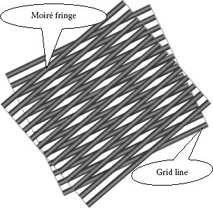
FIGURE 9.1 Superposition of two grid lines and moiré fringe.

In the following sections, we will introduce principle of pattern formation of in-plane and out-ofplane moirés and basic applications to strain analysis and profilometry.

9.2 IN-PLANE MOIRÉ METHOD AND MEASUREMENT OF STRAIN

9.2.1 PATTERN FORMATION OF IN-PLANE MOIRÉ

In-plane moiré pattern is obtained by superposing the reference and the object gratings by direct contact or by imaging one onto the other via a lens. The reference grating has a constant period and fixed spatial orientation, and the object grating is either printed or attached to the object surface. Before deformation of the object, the period and orientation of the object grating are identical to that of the reference grating. Here, let us consider that the object grating is rotated by an angle θ with respect to the reference grating, as shown in Figure 9.1. Seen from a far distance, one no longer can resolve the grating elements, and only see dark and pale bands—moiré pattern. The pale bands correspond to the lines of nodes, namely, elements passing through the intersections of two gratings.

How are the orientation and interval of these moiré patterns in Figure 9.1? Let p and p′ be the periods of the reference and object gratings and φ and d the orientation and interval of moiré pattern, respectively. From geometry, in Figure 9.2,

$O A = \frac{p}{\cos (φ - \frac{π}{2})} = \frac{p}{\sin φ},$ $O A = \frac{p}{\cos (φ - \frac{π}{2})} = \frac{p}{\sin φ},$

(9.1)

$O A = \frac{p^{'}}{\cos (φ - \frac{π}{2} - θ)} = \frac{p^{'}}{\sin (φ - θ)} .$ $O A = \frac{p^{'}}{\cos (φ - \frac{π}{2} - θ)} = \frac{p^{'}}{\sin (φ - θ)} .$

(9.2)

Therefore,

$p^{'} \sin φ = p \sin (φ - θ) .$ $p^{'} \sin φ = p \sin (φ - θ) .$

(9.3)

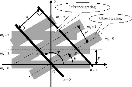
FIGURE 9.2 Order n, orientation φ, and interval d of in-plane moiré pattern; n = m_r − m_o (m_r, m_o are number of reference and object grating elements, respectively).

Rearranging by using geometric functions, we obtain

$φ = \tan^{- 1} \frac{p \sin θ}{p \cos θ - p^{'}} .$ $φ = \tan^{- 1} \frac{p \sin θ}{p \cos θ - p^{'}} .$

(9.4)

From Figure 9.2, we have

$O B = \frac{p}{\sin θ},$ $O B = \frac{p}{\sin θ},$

(9.5)

and

$d = O B \cos (φ - \frac{π}{2} - θ) = O B \sin (φ - θ) .$ $d = O B \cos (φ - \frac{π}{2} - θ) = O B \sin (φ - θ) .$

(9.6)

Substituting Equations 9.3 and 9.5 into Equation 9.6 leads to

$d = \frac{p^{'} \sin φ}{\sin θ} .$ $d = \frac{p^{'} \sin φ}{\sin θ} .$

(9.7)

Rearranging Equation 9.4 by using geometric relationship and then substituting into Equation 9.7 yields

$d = \frac{p p^{'}}{\sqrt{p^{2} \sin^{2} θ + {(p \cos θ - p^{'})}^{2}}} .$ $d = \frac{p p^{'}}{\sqrt{p^{2} \sin^{2} θ + {(p \cos θ - p^{'})}^{2}}} .$

(9.8)

From Equations 9.4 and 9.8, it is obvious that once p, p′, and θ are given, the orientation φ and interval d of the moiré fringe are uniquely decided. Conversely, from the measured values of φ and d, and a given period p of the reference grating, we can obtain the period p′ and orientation θ of the object grating whose structure may be deformed by strains.

9.2.2 APPLICATION TO STRAIN MEASUREMENT

Strain is the geometric expression of deformation caused by the action of stress on an object. Strain is calculated by assuming a change in length or in angle between the beginning and final states. If strain is equal over all parts of the object, it is referred to as homogeneous strain; otherwise, it is inhomogeneous strain. Here, we apply in-plane moiré to measurement of homogeneous linear strain and shear strain.¹,²,³,⁴

9.2.2.1 Linear Strain Measurement

The linear strain ε, according to Eulerian description, is given by

$ε = \frac{δ ℓ}{ℓ_{f}} = \frac{ℓ_{f} - ℓ_{o}}{ℓ_{f}},$ $ε = \frac{δ ℓ}{ℓ_{f}} = \frac{ℓ_{f} - ℓ_{o}}{ℓ_{f}},$

(9.9)

where ℓ_o and ℓ_f are the original and final lengths of the object, respectively. (According to Lagrangian description, the denominator is the original length ℓ_o instead of ℓ_f; for the application of moiré methods, here we use Eulerian description. When the deformation is very small, the difference between the two descriptions is negligible.) The extension δℓ is positive if the object has gained length by tension and negative if it has reduced length by compression. Since ℓ_f is always positive, the sign of linear strain is always the same as the sign of the extension.

In measuring the uniaxial linear strain, the object grating will be printed onto the object surface with its elements perpendicular to the direction of the strain, and the reference grating is superposed on it with the same orientation, as shown in Figure 9.3. Figure 9.3c shows the resultant moiré patterns across the object deformed by the tension. In this case, the period of the object grating will be changed from p to p′, and the orientation of it unchanged, namely, the rotation angle θ in Figure 9.2 is zero.

Substituting θ = 0 into Equation 9.4, the interval d of the moiré fringe becomes

$d = | \frac{p p^{'}}{p - p^{'}} | .$ $d = | \frac{p p^{'}}{p - p^{'}} | .$

(9.10)

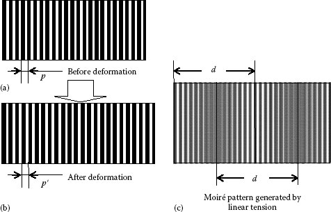
FIGURE 9.3 The reference gating (a) before and (b) after deformation of the object by linear tension and (c) the resultant moiré pattern.

Thus, from Equations 9.9 and 9.10, we obtain the linear strain

$| ε | = | \frac{ℓ_{f} - ℓ_{o}}{ℓ_{f}} | = | \frac{p - p^{'}}{p^{'}} | = \frac{p}{d} .$ $| ε | = | \frac{ℓ_{f} - ℓ_{o}}{ℓ_{f}} | = | \frac{p - p^{'}}{p^{'}} | = \frac{p}{d} .$

(9.11)

Since both p and d are positive magnitudes, the sign of absolute value is introduced to the strain. This means that the appearance of moiré fringe will not explain whether it is a result of tensile or compression strain. To determine the sign of moiré fringe as well as the resulting strain, such techniques as mismatch method and fringe shifting method by translating the reference grating are available.

9.2.2.2 Shear Strain Measurement

The shear strain γ is defined as the angular change between any two lines in an object before and after deformation, assuming that the line lengths are approaching zero. In applying the in-plane moiré method to measure the shear strain, the object grating should be so oriented that its principal direction is parallel to the direction of shear as shown in Figure 9.4a. Figure 9.4b shows typical moiré patterns across the object deformed by the shear. In this deformation, the period p′ of the object grating is assumed same as p before deformation, and the orientation was changed from zero to θ (the quantity of θ is very small). Thus, from Equation 9.8, the interval of the moiré pattern is

$d = \frac{p}{θ} .$ $d = \frac{p}{θ} .$

(9.12)

Comparing Figure 9.4b with Figure 9.2, one can easily see that the shear strain γ is the resulting rotation angle θ of the object grating; hence, it can be expressed by

$γ = \frac{p}{d} .$ $γ = \frac{p}{d} .$

(9.13)

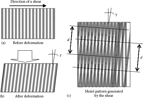
FIGURE 9.4 The reference gating (a) before and (b) after deformation of the object by shear and (c) the resultant moiré pattern.

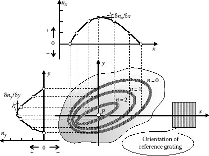
FIGURE 9.5 Strain analysis from 2D moiré fringe.

Although linear and shear strains are discussed independently, in a general 2D deformation, the object grating undergoes rotation as well as change of period with magnitudes varying from place to place, as depicted in Figure 9.5. From this 2D moiré pattern, we obtain linear and shear strains given by

$ε_{x} = p \frac{\partial n_{x}}{\partial x},$ $ε_{x} = p \frac{\partial n_{x}}{\partial x},$

(9.14a)

$ε_{y} = p \frac{\partial n_{y}}{\partial y},$ $ε_{y} = p \frac{\partial n_{y}}{\partial y},$

(9.14b)

$γ = p (\frac{\partial n_{x}}{\partial y} + \frac{\partial n_{y}}{\partial x}),$ $γ = p (\frac{\partial n_{x}}{\partial y} + \frac{\partial n_{y}}{\partial x}),$

(9.14c)

where n_x, n_y are the fringe order at point P along x, y directions, respectively

Gratings used for strain analysis with in-plane moiré method are 20–40 lines/mm and formed by holographic interference technique, e-beam writing, x-ray lithography, phase mast, etc. Object grating is transferred to the object (metal) by lithography using photosensitive coating or photoresist or dichromate gelatin on the object.

9.3 OUT-OF-PLANE MOIRÉ METHOD AND PROFILOMETRY

As mentioned in the previous section, in-plane moiré pattern is generated by superposing the reference and object gratings in the same plane. In applying out-of-plane moiré method to the contour mapping, the object grating formed across the object is distorted in accordance with object profile. This out-of-plane moiré method is also termed moiré topography. The moiré topography is categorized mainly into shadow moiré and projection moiré methods. Shadow moiré method is known as the first example of applying the moiré phenomenon to 3D measurement. (In the early 1970s, H. Takasaki and D. Meadows et al. applied shadow moiré as a technique to the observation of contours on object surface successfully.⁵^,⁶)

Started with the principle of moiré pattern formation of shadow moiré, following sections introduce its application to whole-field measurement and introduce projection moiré.

9.3.1 SHADOW MOIRÉ AND CONTOUR

Shadow moiré pattern is formed between the reference grating and its shadow (the object grating) on the object. The arrangement for shadow moiré is shown in Figure 9.6. The point light source and the detector (the aperture of detector lens is assumed a point) are at a distance l from the reference grating surface and their interseparation is s. Period of the reference grating is p (p ≪ l and p ≪ s). Without loss of generality, we may assume that a point O on the object surface is in contact with the grating. The grating lying over the object surface is illuminated by the point source, and its shadow is projected onto the object. The moiré pattern observed from the detector is the result of superposition between the grating elements contained in OB of the reference grating and the elements contained in OP of the objected grating, which is the shadow of elements contained in OA of the reference grating. Assuming that OA and OB have i and j grating elements, respectively, from the geometry

$A B = O B - O A = j p - i p = n p, n = 0, 1, 2, 3, …$ $A B = O B - O A = j p - i p = n p, n = 0, 1, 2, 3, …$

(9.15)

$A B = h_{n} (\tan α + \tan β),$ $A B = h_{n} (\tan α + \tan β),$

(9.16)

where

n is the order of the moiré pattern

h_n is the depth of nth-order moiré pattern as measured from the reference grating (n = 6 in Figure 9.6)

Hence,

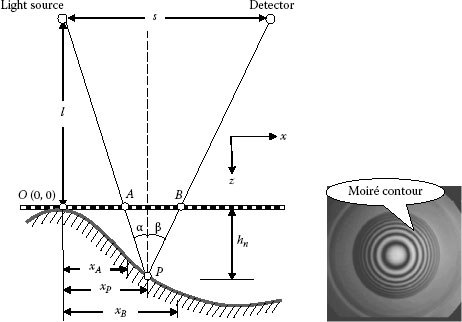
FIGURE 9.6 Optical arrangement of shadow moiré.

$h_{n} = \frac{n p}{\tan α + \tan β} .$ $h_{n} = \frac{n p}{\tan α + \tan β} .$

(9.17)

From Figure 9.6, we also have

$\tan α = \frac{P_{x}}{l + h_{n}} and tan β = \frac{s - x_{P}}{l + h_{n}},$ $\tan α = \frac{P_{x}}{l + h_{n}} and tan β = \frac{s - x_{P}}{l + h_{n}},$

(9.18)

where x_P is x component of OP

Substituting these equations in Equation 9.17 and rearranging lead to

$h_{n} = \frac{n p l}{s - n p} .$ $h_{n} = \frac{n p l}{s - n p} .$

(9.19)

From Equation 9.19, it is seen that the moiré fringes are contours of equal depth measured from the reference grating.

Figure 9.6b shows moiré contour lines on a convex object. Besides these contours, intensity distribution of these moiré fringes also causes interesting result. In practice, knowing the order n of a contour line, we can approximately guess the location of points on the object, and knowing further more about the intensity of that fringe, we can exactly plot measurement point.

9.3.2 INTENSITY OF SHADOW MOIRÉ PATTERN

Before mathematical development of intensity of moiré fringes, let us review about the square wave grating shadow moiré deals with. In Fourier mathematics, it is known that all types of periodic functions (including square wave function) can be described as a sum of simple sinusoidal functions. In shadow moiré, the amplitude transmittance of the square wave grating is considered as that of a sinusoidal grating.

$T (x, y) = \frac{1}{2} + \frac{1}{2} \cos (\frac{2 π}{p} x) .$ $T (x, y) = \frac{1}{2} + \frac{1}{2} \cos (\frac{2 π}{p} x) .$

(9.20)

Then, the resulting intensity at point P is proportional to the product T_A(x_A, y)·T_B(x_B, y).

$I (x, y) = [\frac{1}{2} + \frac{1}{2} \cos (\frac{2 π}{p} x_{A})] [\frac{1}{2} + \frac{1}{2} \cos (\frac{2 π}{p} x_{B})] .$ $I (x, y) = [\frac{1}{2} + \frac{1}{2} \cos (\frac{2 π}{p} x_{A})] [\frac{1}{2} + \frac{1}{2} \cos (\frac{2 π}{p} x_{B})] .$

(9.21)

From Figure 9.6, it is seen that x_A = lx_P/(l + h_P), x_B = (sh_P + lx_P)/(l + h_P). Substituting these equations in Equation 9.21 and rearranging it, we have following normalized intensity:

$I (x, y) = 1 + \cos \frac{2 π}{p} (\frac{l x_{P}}{l + h_{n}}) + \cos \frac{2 π}{p} (\frac{s h_{n} + l x_{P}}{l + h_{n}}) + \frac{1}{2} \cos \frac{2 π}{p} (\frac{2 l x_{P} + s h_{n}}{l + h_{n}}) + \frac{1}{2} \cos \frac{2 π}{p} (\frac{s h_{n}}{l + h_{n}}) .$ $I (x, y) = 1 + \cos \frac{2 π}{p} (\frac{l x_{P}}{l + h_{n}}) + \cos \frac{2 π}{p} (\frac{s h_{n} + l x_{P}}{l + h_{n}}) + \frac{1}{2} \cos \frac{2 π}{p} (\frac{2 l x_{P} + s h_{n}}{l + h_{n}}) + \frac{1}{2} \cos \frac{2 π}{p} (\frac{s h_{n}}{l + h_{n}}) .$

(9.22)

The last term in Equation 9.22 is solely dependent on height and is the contour term. The other three cosine terms representing the reference grating, although height-dependent, are also dependent on x (location) and, hence, do not represent contours. The patterns corresponding to these three terms can obscure the contours as shown in Figure 9.7a. Intensity distribution along cross-sectional line clearly shows the disturbance of the reference grating itself. To remove these unwanted patterns, H. Takasaki proposed, during exposure, to translate the grating in azimuth. The resultant intensity is proportional to

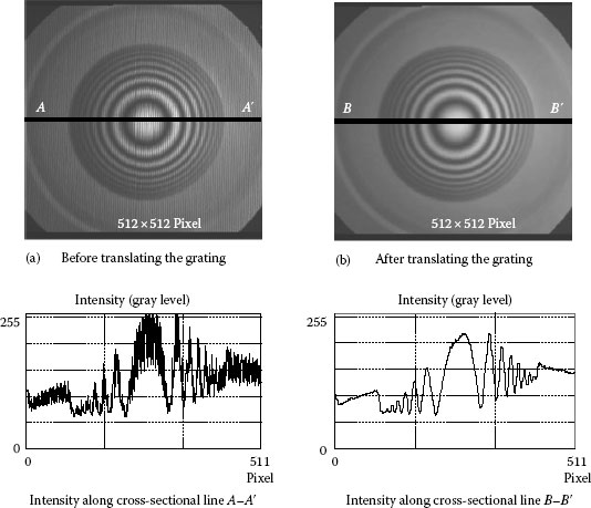
$\begin{array}{l} I (x, y) & = K (x, y) [1 + \frac{1}{2} \cos \frac{2 π}{p} (\frac{s h_{n}}{l + h_{n}})] = a (x, y) + b (x, y) \cos [\frac{2 π}{p} (\frac{s h_{n}}{l + h_{n}})], \\ = a (x, y) + b (x, y) \cos φ (x, y) \end{array}$ $\begin{array}{l} I (x, y) & = K (x, y) [1 + \frac{1}{2} \cos \frac{2 π}{p} (\frac{s h_{n}}{l + h_{n}})] = a (x, y) + b (x, y) \cos [\frac{2 π}{p} (\frac{s h_{n}}{l + h_{n}})], \\ = a (x, y) + b (x, y) \cos φ (x, y) \end{array}$

(9.23)

FIGURE 9.7 Shadow moiré pattern (a) before and (b) after translating the reference grating.

where

a (= K) is the intensity bias

b (= K/2) is the amplitude

φ is the phase related to the temporal phase shift of this cosine variation

The resultant moiré fringes of this equation are shown in Figure 9.7b. Compared with Figure 9.7a, it is obviously seen in Figure 9.7b that the unwanted noise patterns are “mixed out” due to the averaging effect of the reference grating.

When we take pictures, during the exposure, if the object moves, we will get unclear picture. Here, this effect helps us, on the contrary, have clear contour image. Say again, in in-plane moiré method, translating the reference grating is one of important techniques to shift the moiré fringe and then determine the sign and order of the fringe.

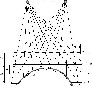
FIGURE 9.8 Relation between phase and the shadow moiré pattern.

Figure 9.8 shows the relations between the phase φ and the moiré contour. The depth h(x, y) of any point P(x, y) on the object surface, then, can be got from the following equation:

$h (x, y) = h_{n} + (h_{n + 1} - h_{n}) [\frac{φ (x, y)}{2 π}] .$ $h (x, y) = h_{n} + (h_{n + 1} - h_{n}) [\frac{φ (x, y)}{2 π}] .$

(9.24)

9.3.3 APPLICATION TO 3D PROFILE MEASUREMENT

To map 3D profiles of objects with shadow moiré topography, phase distribution encoded in intensity distribution can be retrieved from the moiré pattern by using a phase-shifting method.⁷,⁸,⁹,¹⁰,¹¹,¹²,¹³,¹⁴,¹⁵,¹⁶,¹⁷,¹⁸

9.3.3.1 Phase-Shifting Method

In electromagnetic wave interference, the phase-shifting method is well done to get the phase information from modulated intensity. The four-step algorithm is particularly famous for phase calculation in image processing. Here, we apply this algorithm to mechanical interference—moiré. The four-step algorithm to obtain the phase φ in intensity Equation 9.23 is given by

$φ = \tan^{- 1} \frac{I_{3} - I_{1}}{I_{0} - I_{2}},$ $φ = \tan^{- 1} \frac{I_{3} - I_{1}}{I_{0} - I_{2}},$

(9.25)

where I_k is the intensity of the moiré fringes across the object and is described as follows:

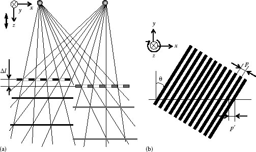
$I_{k} = a + b \cos (φ + \frac{π}{2} k), k = 0, 1, 2, 3.$ $I_{k} = a + b \cos (φ + \frac{π}{2} k), k = 0, 1, 2, 3.$

(9.26)

FIGURE 9.9 (a) Up-and-down movement of the grating and the resultant moiré pattern shift and (b) rotation of the grating.

In shadow moiré, a vertical movement of the grating results in a change of moiré pattern as well as a shift in the phase (see Figure 9.9a). The distance Δh between adjacent moiré fringes (i.e., Δn = 1) can be deduced from Equation 9.19:

$Δ h_{n, n - 1} = h_{n} - h_{n - 1} = \frac{d p l}{(s - n p) [s - (n - 1) p]} .$ $Δ h_{n, n - 1} = h_{n} - h_{n - 1} = \frac{d p l}{(s - n p) [s - (n - 1) p]} .$

(9.27)

Hence, when the quantity of a vertical movement of the grating is Δl, the shifted phase can be expressed as follows:

$2 π \frac{Δ l}{Δ h_{n, n - 1}} = \frac{2 π Δ l (d - n p) [d - (n - 1) p]}{d p l} .$ $2 π \frac{Δ l}{Δ h_{n, n - 1}} = \frac{2 π Δ l (d - n p) [d - (n - 1) p]}{d p l} .$

(9.28)

It is seen that this quantity is not constant but decreases with the order n of moiré contours. Therefore, it is impossible to attain a constant phase change merely by vertical movement of the grating. To keep the phase shift in every order as constant as possible, it is available to rotate the reference grating in addition to move it vertically. Figure 9.9b shows the reference grating rotated, and this rotation results in the variation of the measurement period by

$p^{'} = \frac{p}{\cos θ},$ $p^{'} = \frac{p}{\cos θ},$

(9.29)

where θ is the rotation angle of the reference grating.

The combination of the vertical movement and rotation of the reference grating results in two equations: first, the distance ${h^{'}}_{n}$ ${h^{'}}_{n}$ between the moiré contour of nth order and the reference grating plane, which is transformed from h_n, is given as follows:

${h^{'}}_{n} = \frac{n (l + Δ l) [p / \cos θ]}{s - n [p / \cos θ]} .$ ${h^{'}}_{n} = \frac{n (l + Δ l) [p / \cos θ]}{s - n [p / \cos θ]} .$

(9.30)

Second, the depth h at the point P(x, y) can be expressed with ${h^{'}}_{n}$ ${h^{'}}_{n}$ and Δl under the condition that ${h^{'}}_{n}$ ${h^{'}}_{n}$ exists between h_n and h_n+1:

$\begin{array}{l} h & = h_{n} + (h_{n + 1} - h_{n}) φ / 2 π \\ = {h^{'}}_{n} + Δ l . \end{array}$ $\begin{array}{l} h & = h_{n} + (h_{n + 1} - h_{n}) φ / 2 π \\ = {h^{'}}_{n} + Δ l . \end{array}$

(9.31)

From Equation 9.31, to shift the phase φ by π/2, π, 3π/2, the needed quantities of vertical movement Δl and rotation angle θ of the reference grating are

$Δ l = \frac{φ p l}{2 π (s - p)},$ $Δ l = \frac{φ p l}{2 π (s - p)},$

(9.32)

$θ = \cos^{- 1} (\frac{l}{l + Δ l}) .$ $θ = \cos^{- 1} (\frac{l}{l + Δ l}) .$

(9.33)

Figure 9.10 shows example of four images with phase-shifted moiré patterns and the analyzed results expressed with wire frame.

The limitation of this phase evaluation method is that it cannot be applied to those objects with discontinuous height steps and/or spatially isolated surfaces, because the discontinuities and/or the surface isolations hinder the unique assignment of fringe orders and the unique phase unwrapping.

9.3.3.2 Frequency Sweeping Method

In laser interferometric area, the wavelength shift method is used to measure 3D shapes of objects. Similar concept can be applied to moiré pattern analysis. With this concept, named frequency sweeping, the distance of object from the reference grating plane can be measured by evaluating temporal carrier frequency instead of the phase. Different from the wavelength shift method, this technique changes the grating period p by rotating the grating in different intervals and produces the spatiotemporal moiré patterns.

Let’s think again about Equation 9.23,

$I (x, y) = a (x, y) + b (x, y) \cos [\frac{2 π}{p} (\frac{s h (x, y)}{l + h (x, y)})] .$ $I (x, y) = a (x, y) + b (x, y) \cos [\frac{2 π}{p} (\frac{s h (x, y)}{l + h (x, y)})] .$

(9.34)

Here, 2π/p is defined as the virtual wave number, which is analogous to the wave number k = 2π/λ (λ: wavelength).

As stated in earlier section, when the reference grating is rotated, the measurement grating period of p is changed, namely, the virtual wave number g = 2π/p is changed with time t. By controlling the amount of the rotation angle θ, we can get the following quasi-linear relationship between different virtual wave number and time.

$g (t) = g_{0} + C \cdot t,$ $g (t) = g_{0} + C \cdot t,$

(9.35)

where

C is a constant showing the variation of the virtual wave number

g₀ is the initial virtual wave number 2π/p

Then, Equation 9.34 can be rewritten in the following time-varying form:

$I (x, y; t) = a (x, y; t) + b (x, y; t) \cos [g (t) H (x, y)],$ $I (x, y; t) = a (x, y; t) + b (x, y; t) \cos [g (t) H (x, y)],$

(9.36)

$H (x, y) = [\frac{d h (x, y)}{l + h (x, y)}] .$ $H (x, y) = [\frac{d h (x, y)}{l + h (x, y)}] .$

(9.37)

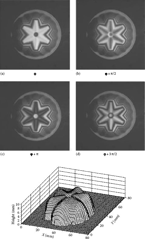
FIGURE 9.10 (a–d) Four images with modulated intensity distribution (a through d) and analyzed result. (With permission of Japan Society for Precision Engineering [35].)

Substituting Equation 9.26 into Equation 9.24 results in the following equation:

$I (x, y; t) = a (x, y; t) + b (x, y; t) \cos [C H (x, y) t + g_{0} H (x, y)] .$ $I (x, y; t) = a (x, y; t) + b (x, y; t) \cos [C H (x, y) t + g_{0} H (x, y)] .$

Here, let us define the temporal carrier frequency f(x, y) as

$f (x, y) = \frac{C \cdot H (x, y)}{2 π},$ $f (x, y) = \frac{C \cdot H (x, y)}{2 π},$

(9.38)

and the second term, initial phase, as

$φ_{0} = g_{0} \cdot H (x, y),$ $φ_{0} = g_{0} \cdot H (x, y),$

(9.39)

then,

$I (x, y; t) = a (x, y; t) + b (x, y; t) \cos [2 π f (x, y) t + φ_{0} (x, y)] .$ $I (x, y; t) = a (x, y; t) + b (x, y; t) \cos [2 π f (x, y) t + φ_{0} (x, y)] .$

(9.40)

As the virtual wave number varies with time t, the intensities at different points vary as shown in Figure 9.11. In this sinusoidal variation, it is obvious that the amounts of the modulated phase φ₀ and the temporal carrier frequency f(x, y) depend on the distance h(x, y) of the object. This means, for the latter, the further the distance, the higher the frequency. Therefore, the height distribution of an object can be obtained from the temporal carrier frequency:

$h (x, y) = \frac{l}{d C / 2 π f (x, y) - 1} .$ $h (x, y) = \frac{l}{d C / 2 π f (x, y) - 1} .$

(9.41)

The frequency f in Equation 9.41 is available by applying fast Fourier transform (FFT) method. Since this frequency sweeping method does not involve phase φ, it is not necessary to carry out the phase-unwrapping process.

Figure 9.12 shows a measurement result, by using the method given earlier, of two objects (ring and rectangle in shape) separated from each other. The period of the grating used for shadow moiré is about 1.0–2.0 mm. The problem of shadow moiré method is that a big grating is necessary for the measurement and the size is dependent on that of objects. The projection moiré method can solve this problem very flexibly by using two gratings.

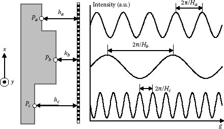
FIGURE 9.11 Relation between the distance h and spatial frequency g.

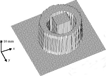
FIGURE 9.12 Measurement result by means of frequency sweeping method. (From Jin, L. et al., Opt. Eng.,40(7), 1383, 2001. With permission.)

9.3.4 PROJECTION MOIRÉ

Projection moiré uses two exactly same gratings: one for projection and the other for reference as shown in Figure 9.13. The projection grating is projected across the object, and the detector captures an image through the reference grating. From Figure 9.13, it is obvious that the principle of moiré pattern formation is completely same as that of shadow moiré. The concepts of phase-shift and frequency sweeping methods are also valuable for projection moiré. For these methods, it just needs to move one of two gratings. The gratings can be easily made of liquid crystal panel plate, or without using any physical gratings, one just projects grating patterns, which is designed with the aid of an application software, through a liquid crystal projector, and then superposes the same grating patterns, inside of the analysis system, on the image with deformed grating patterns.¹⁹ All processes such as shifting the grating and modulating the period can be easily carried on with computer programming.

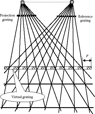
FIGURE 9.13 Principle of projection moiré.

9.4 REFLECTION MOIRÉ

In preceding sections, the moiré technique is performed for strain or profile measurement of diffuse objects. The reflection moiré method can be applied on the objects with mirror-like surfaces.²⁰,²¹,²²,²³ According to how the reflection moiré fringe is obtained, there are several types of reflection moiré method. Figure 9.14 shows one of examples of reflection moiré. The mirror-line surface of the object makes the virtual mirror image of the grating. Then, through the lens, the image of the mirror image of the grating is observed. The moiré fringe can be obtained by exposing double times, before and after deformation of the object, or by placing a reference grating in the image plane of lens. The resulting reflection moiré pattern can be applied to the analysis of slope deformation.

9.5 DIFFRACTION GRATING, INTERFERENCE MOIRÉ, AND APPLICATION

When a holographic grating is illuminated by a monochromatic parallel light beam under an angle of incidence θ₀, between the grating and the object, there occur light beams of zeroth and diffracted higher orders, as shown in Figure 9.15. Namely, the grating acts as diffraction grating. Each beam then interferes with all others. In practice, due to the technique of holographic grating generation, only the zeroth and ±1st orders interfere. The interference pattern formed by the zeroth and first diffraction order has the same period as that of the diffraction grating p. It extends in the direction θ:

$θ = \frac{θ_{0} + θ_{1}}{2},$ $θ = \frac{θ_{0} + θ_{1}}{2},$

(9.42)

where θ₁ is the propagation direction of the first diffraction order beam.

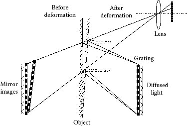
FIGURE 9.14 Principle of reflection moiré.

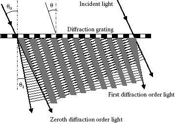
FIGURE 9.15 Interference pattern by diffracted light waves.

According to diffraction theory, the angle θ₁ is given by

$θ = \sin^{- 1} (\frac{λ}{p} + \sin θ_{0}),$ $θ = \sin^{- 1} (\frac{λ}{p} + \sin θ_{0}),$

(9.43)

where λ is the wavelength of incident light.

As depicted in Figure 9.16, the interference pattern is reflected at the surface of the object. The reflected interference pattern will be deformed by the flatness of the object. Through a detector, one can observe moiré fringes superposed by the reflected interference pattern and the diffraction grating (reference grating). From Figure 9.16, for an optical arrangement with parallel illumination and parallel detecting, the distance Δh between two contours can be expressed as

$Δ h = \frac{p}{2 \tan θ} .$ $Δ h = \frac{p}{2 \tan θ} .$

(9.44)

The sensitivity of this method, see from Equation 9.44, will be changed by the incidence angle. This method is also applicable for coherent and incoherent monochromatic light sources, and due to its high sensitivity, moiré method is very attractive for flatness measurement field of such objects as, computer disks, wafers, and smoothly polished glass substrates with highly processed. Figure 9.17 shows a system applying the earlier method to measure flatness of a soda glass substrate. The moiré pattern can be shifted by moving the grating perpendicularly to the objects. Here, the phase-shift method introduced in the previous section can be applied for pattern analysis. In this system, to cancel the influence of the light reflected from the back side of the substrate, an ultraviolet (UV) light (λ = 313 nm) is used as the light source. Part of the UV light will be reflected on the surface of the soda glass, and the left part transmitted into the glass will be absorbed by it. Figure 9.18 shows measurement results by using this system. The grating employed was 10 lines/mm, and the incident angle 60°.

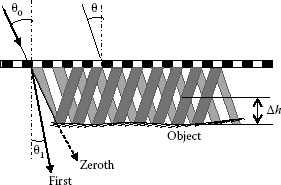
FIGURE 9.16 Generation of moiré pattern.

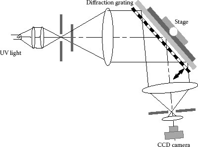
FIGURE 9.17 Flatness measurement system using moiré method.

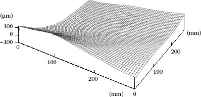
FIGURE 9.18 Measurement result of flatness of a soda glass substrate. (From Fujiwara, H. et al., Proc. SPIE, 2862, 172, 1996. With permission.)

9.6 RECENT TOPICS

As described in the previous sections, moiré phenomenon has been a good topic of research in various fields. Still now we can enjoy moiré produced by overlapping line gratings or random patterns, for example, on the website “http://switzernet.com/people/emin-gabrielyan/070306-paper-moire-basics/paper-eps.pdf (The basics of line moire patterns and optical speedup by Emin Gabrielyan).” At the same time, such an interesting application of moiré as “moiré-based optical tweezers” has been reported. Microparticles and bacteria were trapped and rotated by this idea.²⁴

Regarding moiré applications, we had an opportunity of writing one chapter “Moiré Measurement” in the book.²⁶ We would like to suggest readers who are interested in optical methods for dimensional measurements to read this handbook.

9.6.1 DEVELOPMENT IN SHAPE MEASUREMENT

In electromagnetic wave interference, the phase-shifting method is well done to get the phase information from modulated intensity. The four-step algorithm is particularly famous for phase calculation in image processing. As mentioned in Section 9.3.3.1, mere vertical movement of the grating is not able to invoke a constant phase. To solve this problem, in the early 1990s, Yoshizawa and Tomisawa¹² originally proposed to move the grating vertically and at the same time to translate the light source vertically.

In the arrangement in Figure 9.19, the interval Δh (0.65 mm) is too large to measure the surface profile of the coin (0.25 mm in maximum height). Therefore, phase-shifting technique (that was not popular until 1974) is required to be applied to realize higher sensitivity. They moved the grating vertically by Δl and the light source horizontally by Δd, then four images with mutual phase difference of π/2 are acquired as shown in Figure 9.20. Let us note that one or less than one contour is observed in this case. However, computer processing of these four images (a, b, c, d) using four-step phase-shifting algorithm can produce a representation of the result shown in Figure 9.20e. This method was applied to check damage or wear of a score cap (Figure 9.21a), which is used for die stamping on the top of cans. For the calibration of measurement (Figure 9.21b), cross-sectional profiles obtained by this method (Figure 9.21c) are shown with the result obtained by a mechanical contact profilometer. The two results agree well under the condition that these measurements have to be performed differently.

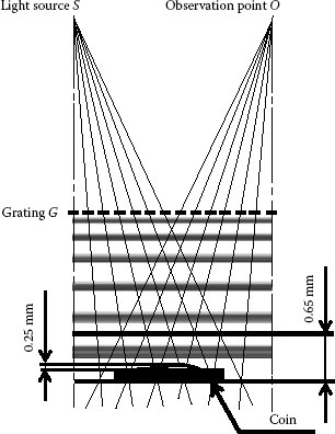
FIGURE 9.19 Arrangement for the surface measurement of a coin.

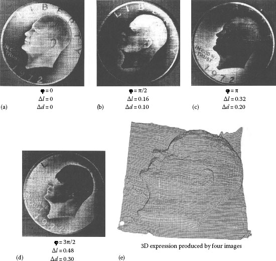
FIGURE 9.20 Four images (a–d) with different phases produce the result (e).

This method was the first trial to apply phase-shifting technique to shadow moiré. However, it was not so easy to use this interesting idea for practical purposes mainly because the devices such as the light source and the grating had to be moved mechanically and manually at that time.

In the case of projection moiré, phase-shifting technique is easily applicable by moving one of separated two gratings, and to get better quality of moiré images, one pair of gratings should be translated at the same speed during the exposure. A primitive proposal was made by Yoshizawa and Yonemura in 1976.²⁶ However, it was not until a few years ago that elements and devices such as liquid crystal gratings, moving stages, and small CCD or CMOS cameras became easily available in addition to PCs. One trial is shown in Figure 9.22, where two linear gratings (G₁ and G₂) are mounted on the motor-controlled translation stages (M₁ and M₂). Relative difference of the phase of gratings that move at constant speed produces heterodyne moiré signal.²⁷ Various ideas were integrated in this arrangement, and one measured example is shown in Figure 9.23. One cross section (Figure 9.24) of the coin proves that accuracy of this method is very high in comparison with the result by a mechanical stylus. Height error was said to be as small as 4.3 μm.

Similar and very refined system was reported by J.J. Dirckx et al. by incorporating such digital devices as the liquid crystal grating and CCD camera. In their arrangement shown in Figure 9.25,²⁸^,²⁹ the green grating (reference grating) is projected on to the sample through the projector lens, and the deformed grating image is formed on the blue-channel liquid crystal light modulating matrix placed outside of the projector with two orthogonal polarizers (second grating). Produced moiré pattern is captured by the CCD camera. In addition to easy phase shift realized by moving one grating, these paired gratings are translated simultaneously to remove grating noise and averaging the “ruling error” of the gratings. This sophisticated system solved various problems inherent to the classical moiré measurement method.

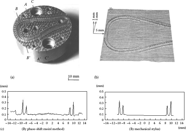
FIGURE 9.21 Checking of score cap: (a) score cap, (b) measurement result, and (c) cross section AA′ by moiré and contact methods.

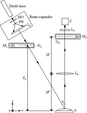
FIGURE 9.22 Optical configuration. S, sample, G₁ and G₂, linear gratings, M₁ and M₂, motorized translation stage [27].

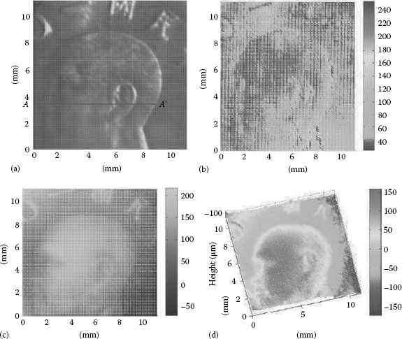
FIGURE 9.23 (a) Sample coin and measured results, (b) moiré fringes, (c) phase map, and (d) reconstructed coin image [27].

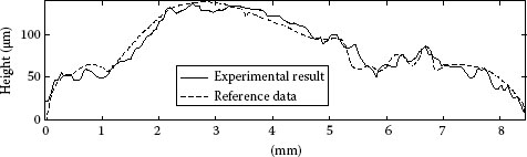
FIGURE 9.24 Cross section AA′. Experimental result and reference data by a stylus method [27].

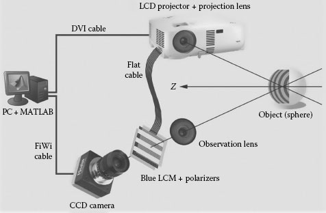
FIGURE 9.25 Setup for digital moiré topography using LCD projector [28,29].

9.6.2 HIGH-SPEED MEASUREMENT

One of the requests to optical methods for industrial purposes is high-speed or, if possible, real-time measurement. In moiré applications, such trial shown in Figure 9.19 may be high in accuracy, but too tedious in operation for practical usage. Not a few techniques have been proposed to solve this problem. Recently, one idea was born that is called as “sampling moiré method.”³¹^–³³ The fundamental principle of this method was reported as early as in 1997 by Arai et al.,³⁰ which aimed to analyze phase distribution of moiré images produced from one-shot image of the deformed grating pattern. At first, this idea was thought just one of “one-shot methods” classified into spatial phase-shifting methods. However, in a subsequent experimental study, the phase distribution of phase-shifted moiré was proved to be analyzed with higher accuracy and higher speed than other methods like FFT method in some cases. This method was applied to analyze 2D grating image. If this principle is used for analyzing 1D grating, it is actually same with the spatial phase analysis based on sampling technique. This sampling method was applied to a dynamically moving object and succeeded in shape measurement as well as strain measurement.

In the sampling moiré method, a specimen grating pattern pasted or drawn on an object is recorded by a digital camera. A specified camera system for this purpose was also developed.³¹ Though the digitized image shows grating, a moiré fringe pattern appears by thinning out the pixels, that is, by sampling the image with a constant pixel pitch. Figure 9.26 illustrates the appearance of moiré fringe patterns by the sampling moiré method. Figure 9.26a shows the deformed grating pattern attached to the specimen. The pitch of the grating in the figure is 1.125 times larger than that of the sampling points. The recorded image is shown in Figure 9.26b, in which no moiré fringe pattern can be discerned. Figure 9.26c shows the moiré fringe patterns when the recorded image is sampled at every Nth pixel (in this case, N = 4). The four images in Figure 9.26c are obtained by using the first, second, third, and fourth pixels of Figure 9.26b as the sampling start point, respectively. This process corresponds to the phase shifting of the fringe pattern. The sampled images shown in Figure 9.26c are interpolated using neighboring data. Then, the four phase-shifted moiré images shown in Figure 9.26d are obtained from one single picture in Figure 9.26b. Phase distribution analyzed from Figure 9.26d is shown in Figure 9.26e. This principle is applicable to the measurement of strain as well as surface shape. Examples are shown in Figures 9.27 and 9.28.³²^,³³ This technique is applicable to capture dynamic objects like a rotating tire and vibrating plates. In the case of mechanical movement of stages or devices, the sampling speed is limited by their moving speed. But in this case, much higher speed is attainable because no mechanical device is used to shift the pattern, that is, to sampling the moiré fringes with continuously changing phase. The next request from industrial fields is the realization of portable and compact equipment, and more and more improvement will be added. From the viewpoint of factory automation, the theses³⁴ are useful and interesting in that it covers such high-speed optical techniques as pattern projection methods (structured light method) in addition to moiré method.

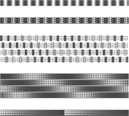
FIGURE 9.26 Principle of sampling moiré method [31,34].

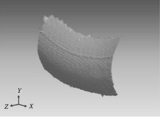
FIGURE 9.27 3D shape measurement of a rotating tire [33].

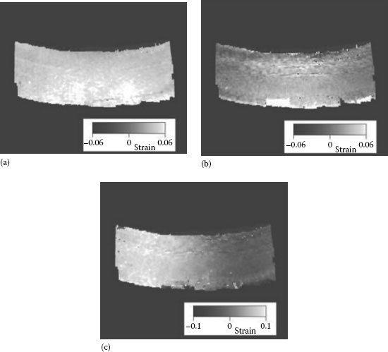
FIGURE 9.28 Measurement result of the strain distribution: (a) in x-direction, (b) in y-direction, and (c) shear strain [33].

9.7 CONCLUSION

Moiré method and applications are described with an emphasis on dimensional measurement and, at the same time, how moiré (originally classical physical phenomenon) has been staying alive for a long time because of its varied characteristics. More different topics can be found in our other review work.²⁵

REFERENCES

1. W. F. Riley and A. J. Durelli, Application of Moiré methods to the determination of transient stress and strain distributions, J. Appl. Mech., 29(1), 23, 1962.

2. F. P. Chiang, On Moiré method applied to the determination of two-dimensional dynamic strain distributions, J. Appl. Mech., Trans. ASME, 39(Series E, 3), 829–830, 1972.

3. F. P. Chiang, V. J. Parks, and A. J. Durelli, Moiré fringe interpolation and multiplication by fringe shifting, Exp. Mech., 8(12), 554–560, 1968.

4. F. P. Chiang, Moiré methods of strain analysis, Exp. Mech., 19(8), 290–308, 1979.

5. H. Takasaki, Moiré topography, Appl. Opt., 9(6), 1467–1472, 1970.

6. D. M. Meadows, W. O. Johnson, and J. B. Allen, Generation of surface contours by moiré patterns, Appl. Opt., 9(4), 942–947, 1970.

7. J. B. Allen and D. M. Meadows, Removal of unwanted patterns from moiré contour maps by grid translation techniques, Appl. Opt., 10(1), 210–213, 1971.

8. L. Pirodda, Shadow and projection moire techniques for absolute or relative mapping of surface shapes, Opt. Eng., 21(4), 640–649, 1982.

9. H. E. Cline, W. E. Lorensen, and A. S. Holik, Automatic moire contouring, Appl. Opt., 23(10), 1454–1459, 1984.

10. V. Srinivasan, H. C. Liu, and M. Halioua, Automated phase-measuring profilometry of 3-D diffuse objects, Appl. Opt., 23(18), 3105–3108, 1984.

11. J. J. J. Dirckx, W. F. Decraemer, and G. Dielis, Phase shift method based on object translation for full field automatic 3-D surface reconstruction from moire topograms, Appl. Opt., 27(6), 1164–1169, 1988.

12. T. Yoshizawa and T. Tomisawa, Shadow moire topography by means of the phase-shift method, Opt. Eng., 32(7), 1668–1674, 1993.

13. G. Mauvoisin, F. Brémand, and A. Lagarde, Three-dimensional shape reconstruction by phase-shifting shadow moiré, Appl. Opt., 33(11), 2163–2169, 1994.

14. Y. Arai, S. Yokozeki, and T. Yamada, Fringe-scanning method using a general function for shadow moiré, Appl. Opt., 34(22), 4877–4882, 1995.

15. X. Xie, J. T. Atkinson, M. J. Lalor, and D. R. Burton, Three-map absolute moiré contouring, Appl. Opt., 35, 6990–6995, 1996.

16. X. Xie, M. J. Lalor, D. R. Burton, and M. M. Shaw, Four-map absolute distance contouring, Opt. Eng., 36(9), 2517–2520, 1997.

17. L. Jin, Y. Kodera, Y. Otani, and T. Yoshizawa, Shadow moiré profilometry using the phase-shifting method, Opt. Eng., 39(8), 2119–2213, 2000.

18. L. Jin, Y. Otani, and T. Yoshizawa, Shadow moiré profilometry using the frequency sweeping, Opt. Eng., 40(7), 1383–1386, 2001.

19. A. Asundi, Projection moire using PSALM, Proc. SPIE, 1554B, 254–265, 1991.

20. F. K. Lichtenberg, The moire method: A new experimental method of the determination of moments in small slab models, Proc. SESA, 12, 83–98, 1955.

21. F. P. Chiang and J. Treiber, A note on Ligtenberg’s reflective moiré method, Exp. Mech., 10(12), 537–538, 1970.

22. W. Jaerisch and G. Makosch, Optical contour mapping of surfaces, Appl. Opt., 12(7), 1552–1557, 1973.

23. H. Fujiwara, Y. Otani, and T. Yoshizawa, Flatness measurement by reflection moiré technique, Proc. SPIE, 2862, 172–176, 1996.

24. P. Zhang, D. Hernandez, D. Cannan, Y. Hu, S. Fardad, S. Huang, J. C. Chen, D. N. Christodoulides, and Z. Chen, Trapping and rotating microparticles and bacteria with moire-based optical propelling beams, Biomed. Opt. Express, 3(8), 1891–1897, 2012.

25. K. Harding, ed., Handbook of Optical Dimensional Metrology, CRC Press (Taylor & Francis), Boca Raton, FL, 2013.

26. T. Yoshizawa and M. Yonemura, Moiré topography with lateral movement of a grating, J. Jpn. Soc. Prec. Eng., 43(5), 556–561, 1976 (in Japanese).

27. W. Chang, F. Hsu, K. Chen, J. Chen, and K. Hsu, Heterodyne moiré surface profilometry, Opt. Express, 22(3), 2845–2852, 2014.

28. J. Buytaert and J. Dirckx, Fringe generation and phase shifting with LCDs in projection moiré topography, Proc. SPIE, 7522, 75220H-1–75220H-8, 2010.

29. J. Dirckx, J. Buytaert, and S. Van der Jeught, Implementation of phase-shifting moiré profilometry on a low cost commercial data projector, Opt. Lasers Eng., 48(2), 244–250, 2010.

30. Y. Arai, S. Yokozeki, K. Shiraki, and T. Yamada, High precision two-dimensional spatial fringe analysis method, J. Mod. Opt., 44(4), 739–751, 1997.

31. M. Fujigaki, Y. Morimoto, and Q. Gao, Shape and displacement measurement by phase-shifting scanning moiré method using digital micro-mirror device, Proc. SPIE, 4537, 362–365, 2002.

32. M. Fujigaki, Y. Sasatani, A. Masaya, H. Kondo, M. Nakabo, T. Hara, Y. Morimoto, D. Asai, T. Miyagi, and N. Kurokawa, Development of sampling moiré camera for real-time phase analysis, Appl. Mech. Mater., 83, 48–53, 2011.

33. M. Fujigaki, K. Shimo, A. Masaya, and Y. Morimoto, Dynamic shape and strain measurements of rotating tire using a sampling moiré method, Opt. Eng., 50(10), 101506–1–101506–8, 2011.

34. D. Asai, Speeding up 3D measurement with phase shifting grating projection in factory automation, Doctor thesis, Wakayama University, Wakayama, Japan, March 2014 (in Japanese).

35. Y. Kodera, L. Jin, Y. Otani, and T. Yoshizawa, Shadow moire profilometry using phase shifting method, J. Precision Eng., 65(10), 1455, 1999 (in Japanese).

..................Content has been hidden....................

You can't read the all page of ebook, please click here login for view all page.

Table of Contents for Chapter 9 Moiré Metrology

Create new playlist

Sign In

Sign Up

Table of Contents for
Chapter 9 Moiré Metrology